1. Introduction
The Ethiopian Highlands provide the resource base for millions of people from the headwaters of the Blue Nile (Abay) to Egypt’s Delta. In Ethiopia, the mountains are blanketed with rich soil and are heavily cultivated from top to bottom. By intercepting the precipitation associated with the monsoon winds of the Indian Ocean, the highlands form the headwaters of the Blue Nile. With an expanding population and the associated intensive land use practices, the highlands are also increasingly under pressure such that land degradation in the form of erosion and topsoil loss is now widespread. Indeed, extensive land degradation, combined with climate variability, is often implicated in the food shortages experienced in Ethiopia in the 1970s and 1980s [
1]. Soil erosion that results in land degradation also threatens water quality and quantity in downstream countries by increasing sedimentation in low-lying areas of Sudan as well as accelerating the siltation of the great Aswan Dam in Egypt. With projected increases in population and changes in climate, a crisis in the highlands is looming and requires quantitative and reliable environmental assessments of the landscape. Land cover data and cropland extent are essential for this assessment, especially in regions facing food security challenges [
2,
3]. However, despite this pressing need for environmental evaluation, monitoring and simulation, there are few datasets of high quality observations on the status of the landscape in this region that could serve as input to these applications, at the spatial resolution of the smallholder farming livelihood. This follows the general trend that even important areas for mapping do not receive sufficient attention when they are located in difficult-to-map areas [
4].
There are global and regional land cover products that encompass Ethiopia and East Africa for some time. Africover provides 30 m spatial resolution and uses the comprehensive UN Land Cover Classification System (LCCS), but it is unavailable for Ethiopia [
5]. Global Land Cover 2000 (GLC2000) uses daily observations of Satellite Pour l’Observation de la Terre-4 (SPOT4) VEGETATION sensor and divides the globe into regions which are classified individually in partnership with regional experts using unsupervised classification methods. Using LCCS, the detailed land cover categories of the regional maps are aggregated into more general types for production of a global land cover map all with a spatial resolution of 1 km [
6]. Also at 1-km resolution, the Collection 4 moderate-resolution imaging spectroradiometer (MODIS) Global Land Cover Map uses a supervised classification with a boosted decision tree and maintains a database of geographically dispersed, representative sites for each land cover class. It immediately provided improved information compared to AVHRR derived land cover products [
7]. Then, Collection 5 of MODIS Land Cover upgraded the input data and the ensemble decision tree algorithm used to classify those data to produce an improved map at higher spatial resolution (500 m) [
8]. Comparisons of the 1 km resolution global land cover products have found broad agreement over much of the globe. Challenges remain in the areas of disagreement such as mixed covers, savannah and shrublands leading to the conclusion that improving mapping of heterogeneous landscapes is of paramount importance [
9,
10].
More recently, a global, Landsat-based, 30 m spatial resolution product called Finer Resolution and Monitoring of Global Land Cover (FROM-GLC) has been produced [
11]. This land cover map was developed by first testing four classifiers, SVM, Random Forest, Maximum Likelihood Classifier and a decision tree and using Landsat TM and ETM+ as input spectral data [
11]. In a follow-up study, using Improved FROM-GLC, this map was further improved by the addition of MODIS-derived EVI, monthly climate data, a digital elevation model, and soil-water status as well as the use of a segmentation algorithm [
12]. The whole map, but especially the cropland class, benefited from the addition of greater temporal information. This new 30-m resolution map is a boon to environmental monitoring applications but it still experiences some difficulty with the heterogeneous landscapes of Africa, and Ethiopia has among the lowest accuracy within the map [
11]. It is this specific deficiency this study seeks to address.
Significant work has also focused on understanding the distribution of global cropland and, some of it, leverages the land cover products detailed above. Comparing MODIS land cover and GLC2000 with regards to cropland, MODIS estimates of crops tend to underestimate total agricultural area whereas GLC-2000 tends to overestimate cropping area [
13]. Using MODIS data, cropland was mapped globally using a probability thresholding technique per country in combination with national agricultural statistics. The map produced at 250 m was generally successful in areas of intensive corn and soybean production but challenged in areas of lower agricultural intensity like Africa [
14]. For sub-Saharan Africa, a map of crops and no crops was created using GLC2000, MODIS Land Cover, GlobCover, MODIS Crop Likelihood and AfriCover and a synergy approach which ranked the land cover products to give a confidence score per pixel which was then combined with national and sub-national statistics. It achieved high overall accuracy for the map at >80% but also errors of omission at ~60% and errors of commission at ~50% for the crop class at a 1-km pixel size [
15]. Very recently, a cropland mask for Africa was created at 250-m resolution by combining results from various land cover products including Africover as well as national and sub-National land cover maps in some areas. The results were judged to be an improvement from the global crop mask and African crop mask mentioned above [
16].
Many of the state-of-the-art techniques from large scale global and regional land cover mapping have also been used along with other remote sensing tools and methods in land use and land cover change studies addressing the difficulty of mapping specific heterogeneous and smallholder agricultural landscapes like those of the Ethiopian highlands. One land cover study which attempts to map cropping areas of central Ethiopia achieved overall accuracy of 55%–74% for its agricultural classes that were differentiated based on intensity of cropping by supplementing wide area use of Landsat TM data with limited area use of 1-m resolution IKONOS imagery [
17]. In a single district of Zimbabwe, an area of about 2000 km
2, land cover mapping through a combined method of unsupervised and supervised classification schemes achieved 85% accuracy including within agriculture but much of that is large-scale commercial agriculture [
18]. A dense time stack of imagery for a single year coupled with phenological curves fed into a decision tree was important in discerning irrigated from rainfed agriculture in West Africa, but there was still difficulty in separating rainfed agriculture from natural vegetation in the heterogeneous smallholder landscape [
19]. These authors point to the need for greater temporal information and the utility of machine learning algorithms combined with other ancillary datasets as the next steps towards addressing these challenges. Topographic information proved useful for land cover change assessment in a difficult mixed wetland and smallholder landscape of Uganda. By adding a digital elevation model (DEM) and slope from 90 m Shuttle Radar Topography Mission (SRTM), the authors were better able to understand land use change trends around Kibale National Park [
20]. For a study area in southern Zambia, one study significantly improved on their objective of identifying cropped areas when they decreased errors of commission by probabilistic reclassification using a logit model [
21]. Most recently, swidden agriculture in Southeast Asia has been mapped with Landsat 8 and a thresholding strategy using several spectral based indices [
22].
The purpose of the research presented here is to document the details of a new land cover map of high spatial resolution for an area of high mapping complexity and important environmental value, the Ethiopian highlands. This map is derived from remotely sensed observations and developed in support of soil erosion, digital soil mapping and crop modeling studies. The method used to develop the map combine many of the techniques from the studies above in order to address the deficiency of available, high-quality land cover mapping for these important agricultural highlands. Our goal is to describe the procedures used to develop this map, its attributes, its reliability, and its applications for environmental assessment and simulation in the region. In the following sections, we describe the geographic setting of the highlands, attributes of the remotely sensed data inputs, the mapping procedure, and the accuracy assessment.
2. Materials and Methods
2.1. Study Area
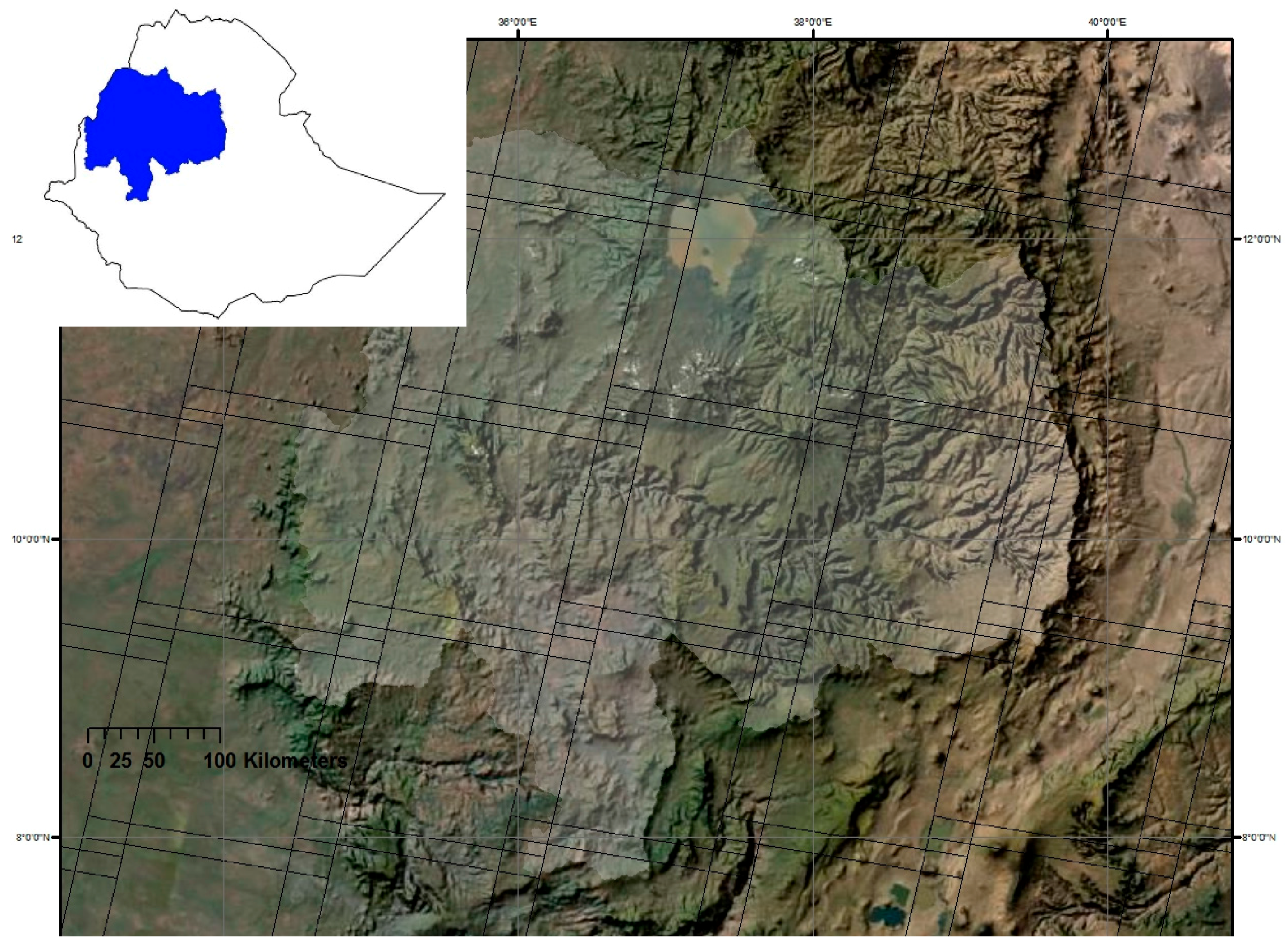
The Ethiopian Highlands are a rugged mass of mountains covering much of central and northern Ethiopia. Our study area is located in the northwestern portion of the Highlands in an area bounded roughly by 8°–12°N latitude and 34.5°–39.5°E longitude. Our site, an area covering 20,000 km
2 to the north and west of the capital, Addis Ababa, includes wet highlands that reach 4000 m above sea level, a small portion of the Rift Valley below the Eastern Escarpment at 500 m elevation, and foot slopes to the highlands in the west all the way to the Ethiopian border with Sudan. The main topographic feature of the study site is the Choke Mountain Range in the center, which is encircled by the Blue Nile as it winds southeast from Lake Tana and then heads west toward Sudan (
Figure 1). Rainfall in the highlands is mainly during the wet season from July to September and is characterized by high intensity storms. Generally, rainfall varies with altitude and east to west, with typical annual totals from 400 to 1500 mm with higher totals seen in the west and highest altitudes (>3000 m above sea level (masl)) and lower totals in the east and in the gorge around Choke Mountain (<1000 masl) [
23].
The study area is contained in the Amhara region for the most part, with small portions of the regions of Oromo, Afar, and Benishangul-Gumuz in the watershed. Rainfed cereal agriculture dominates the highlands with barley, wheat and teff being among the most important crops. Others include millet, sorghum, maize, chickpeas and other legumes. Important non-grain crops cultivated in fields or home gardens are potatoes, garlic, onions, tomatoes, and peppers. The Ethiopian society is largely agrarian with agriculture accounting for 48% of GDP and 85% of employment [
24], but there are few data on how much land is under cultivation.
Livestock husbandry is an important component of rural livelihoods in the study area. Serpentine grasslands lie along bottomlands among the grain fields of the agricultural plateaus and valleys of the highlands. These grazing areas have rules of access typically established at the community level. Cattle, sheep and goats are the most common ruminants in highland agricultural systems. Additional fodder that is important in the grazing system includes crop residues and flora found on hill slopes.
The citizens of Amhara are mostly Ethiopian Orthodox Christians; they represent over 95% of the population according to the last census [
25]. The many Ethiopian Orthodox churches that dot the highlands protect some of the healthiest portions of forest in the study area. Besides these, tree cover in the highlands is limited to community and individual woodlots (often in Eucalyptus) or inaccessible areas. Erosion of highland soil is often attributed in part to this lack of tree and shrub cover as well as overgrazing and the intensity and methods of cultivation [
1].
2.2. Data
Landsat-5 Thematic Mapper (TM) and Landsat-7 Enhanced Thematic Mapper Plus (ETM+) are excellent sensors for the project because of their spectral, spatial and temporal coverage. The spectral bands in red, near infra-red and shortwave infra-red are well suited to identifying vegetative land covers over large areas. The relatively fine spatial resolution (30 m) allows identification of landscape features that are critical in further agriculture and other environmental monitoring studies [
26]. Additionally, the deep (and free) temporal archive of Landsat imagery is essential for capturing phenological differences among the various vegetative land cover classes. For instance, agriculture greens up and dies back in the course of the growing season whereas forest maintains high level of greenness all year.
Several hundred individual scenes that had been acquired by both Landsat-5 TM and Landsat-7 ETM+ instruments covering a total of 14 individual footprints as part of the second World Reference System grid were downloaded from the United States Geological Survey (USGS) Earth Explorer system (
Table 1). The image acquisition period covered a wide range from 2000 to 2011. Due to the Scan Line Corrector (SLC-Off) issue associated with the ETM+ instrument, Landsat 5 images from 2008 to 2011 were preferred when cloud free images were available. Note that the climate of the study area is dominated by the African monsoon system that leads to persistent cloud cover over a significant portion of the year. Unfortunately, this is also the period when most crops are grown. To remedy this issue, we decided to expand the number of years that are included in the study. The rationale behind using this wide range of dates was to increase the likelihood of having cloud-free images within the monsoon period. Note that the time period of 10+ years used here could be seen as excessively long for a static land cover mapping exercise. Nevertheless, as shown in
Table 1, the majority of the images were from the 2008–2011 period, although the time window started in 2000. Often, in order to gather at least 10 distinct dates of imagery for each path/row, Landsat-5 and Landsat 7 data from 2000 to 2003 were also used. We attempted to find cloud free data from a variety of times of the year for several years, but generally cloud cover up to about 25% had to be accepted in order to obtain some data from the rainy season.
The second source of data was a 30-m spatial resolution DEM derived from the Advanced Spaceborne Thermal Emission Radiometer (ASTER) observations [
27]. The DEM dataset provided an important non-spectral input for this classification by characterizing elevation and slope-related landscape variability, particularly in two classes of interest. In the agriculture class, crop types are expected to vary with elevation as well as crop calendar. In dryer lowlands, grassy areas may green up only for a brief period during and immediately after the wet season, causing them to be spectrally similar to grain crops on higher plateaus. Woody vegetation varies with rainfall, which changes with elevation, but at the highest elevations woody cover gives way to grassland. By adding the DEM, the classifier was enabled to discriminate between some classes and aggregate within a varied class. In addition, slope information was derived from the DEM, which helped improve separability between classes. For example, spectral discrimination among the grassland, agriculture, and wooded categories in Ethiopian highlands is often very difficult. However, since Ethiopian law bans cultivation on slopes greater than 20 degrees, the steepest vegetated slopes are expected to be occupied by grasslands rather than agricultural cover. The flattest, lowest areas are often ribbons of managed pasture among a sea of cereal agriculture.
2.3. Pre-Processing
A cloud mask was applied to each image with greater than 5% cloud cover. This mask removed the clouds and their shadows from the six reflective bands. We used a common cloud detection algorithm called FMask [
28]. Nearly all images, even those acquired in the dry season, had at least 5% cloud cover. The wet season imagery often exceeded 20% cloud cover, but images with more than 35% cloud cover were excluded. Our intent was to find enough imagery for each season to have spatial and temporal coverage in spite of the “holes” created by the masking process.
The Landsat data were not atmospherically corrected, since each footprint was classified individually using an approach in which all available cloud-screened raw data, together with derived vegetation index and topographic information, were classified as a single large image stack. The DEM was trimmed to match each path/row, and finally, these DEM data were used to generate slope based on a 5 × 5 pixel moving window.
In addition to the raw spectral input, we also derived Normalized Difference Vegetation Indices (NDVI) from the original Landsat data using the following well-known formula:
where
NIR and
R correspond to near-infrared and red spectral bands of Landsat, respectively. These derived
NDVI layers for each date were made from the cloud-masked layers.
The logical extreme of the masking process is an area where cloud cover is complete throughout the image stack, which would lead to a set of pixels with no spectral input to the classifier. In this case, slope and DEM would be the only nonzero data for determining land cover. In reality, the top of Choke Mountain itself is the only area with such ubiquitous cloud cover (and it is not complete across all the dates of imagery). At the top of the mountain, the cover is nearly all grass and slope and DEM alone would give the classifier reasonable likelihood of making the correct determination.
2.4. Classification Scheme
The most difficult part of classification was dealing with variability and mixed pixels across the landscape at Landsat’s 30-m resolution. Class labels were chosen to include the major broad categories of land use and cover. The land cover classes included: agriculture, bare ground, urban/impervious surfaces, grasslands, marsh and seasonal water, water, wooded/shrub and forest areas.
Table 2 outlines the features of these classes.
Agriculture in the study area most often consists of a patchwork of smallholder plots in valleys and on mountainsides with very few areas of larger, broad tracts of mechanized production. The growing season is generally from July to December for the major grain crops. The most important grains in the highlands are wheat, barley and the indigenous grain teff. At higher elevations, potatoes are common and often rotated with barley. At lower elevations below the escarpment on the western edge of the study area, peanuts are common and there is much more maize.
The grassland class covers bottomland pasture of the highlands, herbaceous high mountain meadows, grassy mountainside and some extensive savannah grasslands of the lowlands. This includes a wide range of productivity. Rich, well-managed pasture of the highlands and extensive savannah in the west of the study area may be green for much of the year. On the other hand, on the foot slopes toward the Afar basin at the eastern edge of the study area, semi-arid grasslands may green up for only a short period after limited rains. This class also includes areas where up to 30% is covered in woody plants, shrubs and trees.
The wooded class represents a variety of savannah-like land cover seen in both the highlands and lowlands. Hillsides and river canyons are often covered in dense shrub and are one example of this class. The wooded class includes areas that range from >30% shrub or tree cover up to dense, closed canopy forest seen only in the western lowlands. The forest class, then, is found mostly in the west region of the study area. The highlands have limited forest cover in protected church forests, inaccessible areas of the mountains, and community and individual woodlots (often a Eucalyptus variety).
The bare ground class contains eroded and degraded hillsides, pasture or farmland, village lands, some dry riverbeds and arid areas in the east. The urban/impervious surface class encompasses urban areas, other built structures, and bare rock. Finally, marsh and seasonal water are seen in only a few locales, near dams and where bottom lands are prone to flooding.
2.5. Classification Inputs
Most stacks of images included more than 100 bands. Most of the bands in the image stacks contained the raw Digital Number (DN) from Landsat’s reflective bands. The slope and elevation derived from the digital elevation model were also included in all image stacks. Note that a test case using both the Top of the Atmosphere (TOA) and Surface Reflectance inputs and derived vegetation index did not produce improved classification results and hence only DN inputs were used in the classification process.
Vegetation indices over time can be useful in classifications, so from the set of NDVI images, the mean and variance at each pixel in those bands were calculated to create a temporally longitudinal data layer. The result was two additional bands of data, one for mean and one for variance of NDVI for each Landsat path/row. Finally, all these bands were combined into a single image stack for each path/row for use by the classifier.
In two cases, path/row 170/52 and 168/52, the image stack was segmented by elevation in order to run it through the classifier with separate training data for highlands and lowlands. In both of these areas, an escarpment bisects the scene, separating significantly different agroecologies. An elevation mask was created for areas greater and less than 1500 masl. The choice of 1500 masl is not an arbitrary number. Inspection of the DEM at the escarpment boundary shows a sharp change around 1500 m, and this is in line with Ethiopian agricultural nomenclature for the transition from Kolla (lowlands) to Weina Dega (low highlands) [
1]. Training data for these two elevation bands were gathered separately and the classifiers run separately.
2.6. Classification Algorithm
The variability seen in Ethiopia’s agrarian landscape required a classification algorithm equipped to deal with complex relationships between spectral inputs afforded by satellite data and land surface conditions while being immune to missing or mislabeled training data. In this research, we chose a Support Vector Machines (SVM) algorithm for this task. SVM is a supervised, non-parametric statistical learning technique that has been shown to be appropriate for classification problems with large dimensionality [
29]. The SVM algorithm works by determining, through an iterative learning process, an optimal linear hyperplane of
N-dimensional space that separates the input data into the predefined classes [
30,
31].
SVMs are known to be especially well-suited for applications of multispectral remote sensing [
29,
31,
32]. The support vectors are defined using only a subset of the training data. Those that lie on the margin are used to define the hyperplane of maximum margin, which allows SVMs to handle small training sets [
33]. SVMs are less data intensive than other machine learning algorithms such as Artificial Neural Networks, which require additional training data as the input dimensionality increases [
32]. Finally, when input spectral data are not normally distributed, the SVM algorithm is superior to classifiers such as the Maximum Likelihood Classification, which require a normal distribution of data [
29].
Several approaches have been developed to improve SVM predictive accuracies using multispectral remote sensing data. These include the soft margin approach and kernel-based learning that lead to SVM optimization in higher learning space, although the kernel functions often result in more expensive parameterization [
34,
35,
36]. Note that while SVMs have been shown to perform well in spite of a certain level of noise (i.e., mislabeled training data), they are not completely impervious to outliers [
37]. Methods have been developed to mitigate the effects of outliers on SVMs that include assigning a confidence value that indicates how likely a point is believed to be an outlier, or through fuzzy-SVMs and weighted-SVMs [
37,
38,
39,
40]. However, these studies show only incremental improvements over standard SVM methods [
38]. With sufficient ground truth information and large amounts of satellite data over time, the SVM algorithm should be able to be trained to separate classes of the Ethiopian landscape in spite of their great inherent variability.
To show that SVMs were the right tool for this classification problem, we further evaluated four different image classification algorithms, namely the Maximum Likelihood, Decision Trees, Neural Networks, and K-nearest neighbor algorithm. To achieve this, we picked a footprint that appeared to have the most diverse set of land cover types and used the training data associated with that footprint and used a 10-fold cross validation procedure with 75/25 training/testing split. This preliminary analysis (not shown) confirmed that in Ethiopia’s complex agrarian landscapes, SVMs outperformed other image classification algorithms. The SVM classifier was able to remove both the striping artifacts in the final classification results associated with the Landsat 7 SLC-Off issue and the salt-and-pepper texture common in per pixel classification results. The SVM classification was 5–25 percent higher in overall accuracy without a significant computation cost. Three reasons contribute to this, which have already been identified in the literature. First, regardless of the size of the learning sample, not all the available examples are used in the specification of the hyperplane. This allows SVMs to successfully handle small training data sets because only a subset of points that lie on the margin—the support vectors—are used to define the hyperplane [
33]. Second, unlike many statistical classifiers, SVMs do not make prior assumptions on the probability distribution of the data, and this leads to reduction in classification errors when input data do not conform to a distribution that other statistical qualifiers may require (e.g., Gaussian). Third, SVM-based classification algorithms have been shown to produce generalizable models from a set of input training data, eliminating the notion of overfitting [
41].
2.7. Training Data
The method for collecting training data was manual interpretation of the original Landsat data, supplemented by high-resolution imagery available through Google Earth. There is a growing number of high-resolution images, even covering areas of rural Ethiopia, available in Google Earth. A typical training data collection exercise takes the following form: first, the analyst displays several dates of Landsat imagery, usually one or two from the dry season and one or two from the rainy season, and possibly another one or two that seem particularly helpful for a given class. Displaying many images allows the analyst to see the phenological changes, which aid in the recognition of different land cover types. The analyst then finds a target land cover in the scene and confirms that land cover by cross-referencing the area in Google Earth’s imagery. For homogenous classes like water, only a couple of hundred pixels per footprint were gathered for training. In some areas of the Landsat scenes, availability of multiple dates of high resolution data in Google Earth make it easier to interpret the landscape. For more complicated classes, such as agriculture and wooded categories, 1000–2000 pixels are chosen in each Landsat path/row with an average total of ~5000 training pixels for each Landsat scene across the eight land cover classes. These training pixels are gathered for each of the 14 Landsat scenes individually, and finally the SVM tool is run for each Landsat scene separately.
After running the classifier, results are assessed visually to compare assigned classes to an analyst’s interpretation of raw data and Google Earth imagery. New training data are gathered via this method for several iterations of the classification before formal accuracy assessment is undertaken. Once the analyst is satisfied with the results qualitatively, an image segmentation and accuracy assessment can be performed (see below). With this objective feedback, the analyst may continue to gather training data to improve the most troublesome classes. Each Landsat footprint requires somewhere between four and eight iterations before the classification is considered final.
2.8. Refinement of Wooded Cover Categories
Our preliminary accuracy assessment indicated that there was great confusion between the wooded/shrub category and forested areas, especially in lower woody covered sites. To remedy this, we used an independent (i.e., it was not part of SVM classification inputs) continuous forest cover dataset and a thresholding approach to more accurately separate the shrub category from the forest category. In particular, we used the Landsat Vegetation Continuous Fields (VCF) tree cover dataset [
42] that contains estimates of the percentage of horizontal ground in each 30 m pixel covered by woody vegetation greater than 5 m in height. The VCF data were for the 2005 target year and developed from the NASA/USGS Global Land Survey collection (GLS) of Landsat data [
42].
Note that although the Landsat VCF product was designed to capture woody land cover fractions, we noticed that very low values of VCF observations were required to identify large fractions of actual woody cover. Specifically, when an independent set of wooded areal fractions data—extracted by visual examination of a set of randomly located 90 m × 90 m samples—was compared to the VCF data for the same plots, a small range of VCF values (0%–30%) covered the full range of wooded fractions (0%–90%). This finding required that we translate the original VCF data to a new range of woody cover areal fraction data using a logistic fit. The new “scaled” range of VCF values (VCFscaled) then allowed for better separation of the shrubland category (VCFscaled ≤ 50%) from the forested category (VCFscaled > 50%). In the final land cover map, the original shrubland and forest categories were then replaced with this independent two-category dataset derived from the scaled Landsat VCF data.
2.9. Post-Processing—Image Segmentation
Raw outputs from a classification algorithm often contain significant noise when examined on a pixel-by-pixel basis. To overcome this issue, we employed a post-classification segmentation process to translate the initial per-pixel results to per-polygon outcomes (segments). To do this, we employed a segmentation algorithm [
43] with a minimum mapping unit of six Landsat pixels (roughly equal to 0.5 hectares). Input features to the segmentation tool included a combination of Landsat bands 3, 4, and 5 images (red, NIR, and SWIR) from a set of dates that maximized both the number of valid observations (defined as free of cloud, cloud shadows, and SLC-Off gaps) and the temporal variability. These inputs typically included at least one image from the wet season and at least one from the dry period. Per-pixel classification results were first eroded and dilated, and converted to polygon-based outputs using a simple plurality (majority) rule. The final polygon-based classified images were more realistic and devoid of the high frequency noise present in the original per-pixel classification results. After adding in clouds and cloud shadows that were masked out earlier, each footprint contained a final land cover map in vector format. Note that the cloud/cloud shadow categories only exist in a small number of locations and hence they are not seen as a hindrance to the land cover map produced here. The final fourteen maps were then merged to make a single land cover map covering over 96% of the Abay Basin.
2.10. Accuracy Assessment
The accuracy of the final map was evaluated using two different methods associated with two independent validation datasets. In the first method, all categories of the final classification were assessed for accuracy by using random sampling. Roughly 200 segments per category were chosen. These segments were then assessed by an analyst through visual inspection of the vector overlays within Google Earth. In the end, the total number of independent samples was in excess of 1450. Note that while it would have been desirable to use a ground-validated dataset to assess the accuracy of the land cover maps, neither the data nor the resources to evaluate the entire area of the study were available or logistically feasible. In the final step, the independent set of samples was used to generate a confusion matrix, a standard tool for quantifying map accuracy derived from remotely sensed data [
44].
In the second method, we evaluated only the cropland category against all other categories using an existing validation set acquired as part of the Geo-Wiki project [
45] As part of a global land cover validation exercise, the Geo-Wiki team assembled a volunteer basis crop/non-crop dataset for all of Ethiopia in 2012. Each analyst was asked to identify a randomly selected location for crop presence along with the degree of presence as well as confidence in making a decision. For this evaluation purpose, we selected roughly equal amounts of crop and non-crop samples covering only the study area (the Abay Basin) from the large Ethiopia-wide dataset. We then compared the observed (reference) label of each sample to the map label and summarized the results in a confusion matrix.
3. Results
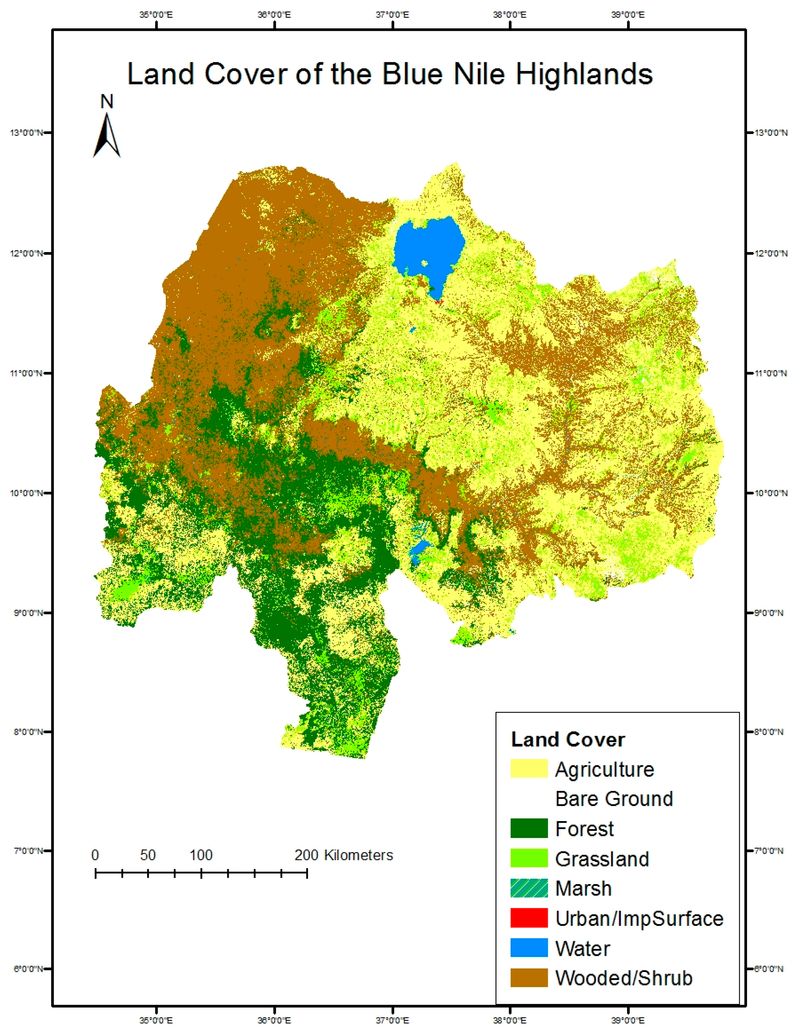
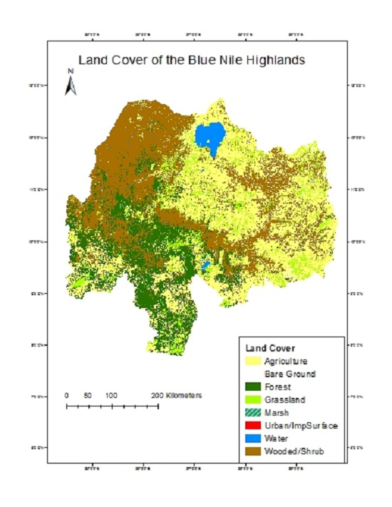
Visual assessment of the results on the final map (
Figure 2) shows that some broad relationships were well captured by the classification. A general look at the results shows ~35% of the area (~7,000,000 ha) is occupied by agriculture, which is slightly more than wooded/shrub which covers 33% of the map. Agriculture dominates the highlands of Amhara and Oromo in the center of the map and becomes sparse in the western lowlands, which are humid but characterized by more extensive production systems. The patterns of pasture and farmland throughout the agricultural plateau will be especially important for erosion studies and can be seen in
Figure 3 and
Figure 4. The farmland in the highlands is often threaded with tendrils of managed pasture in the flattest and lowest areas of village territories.
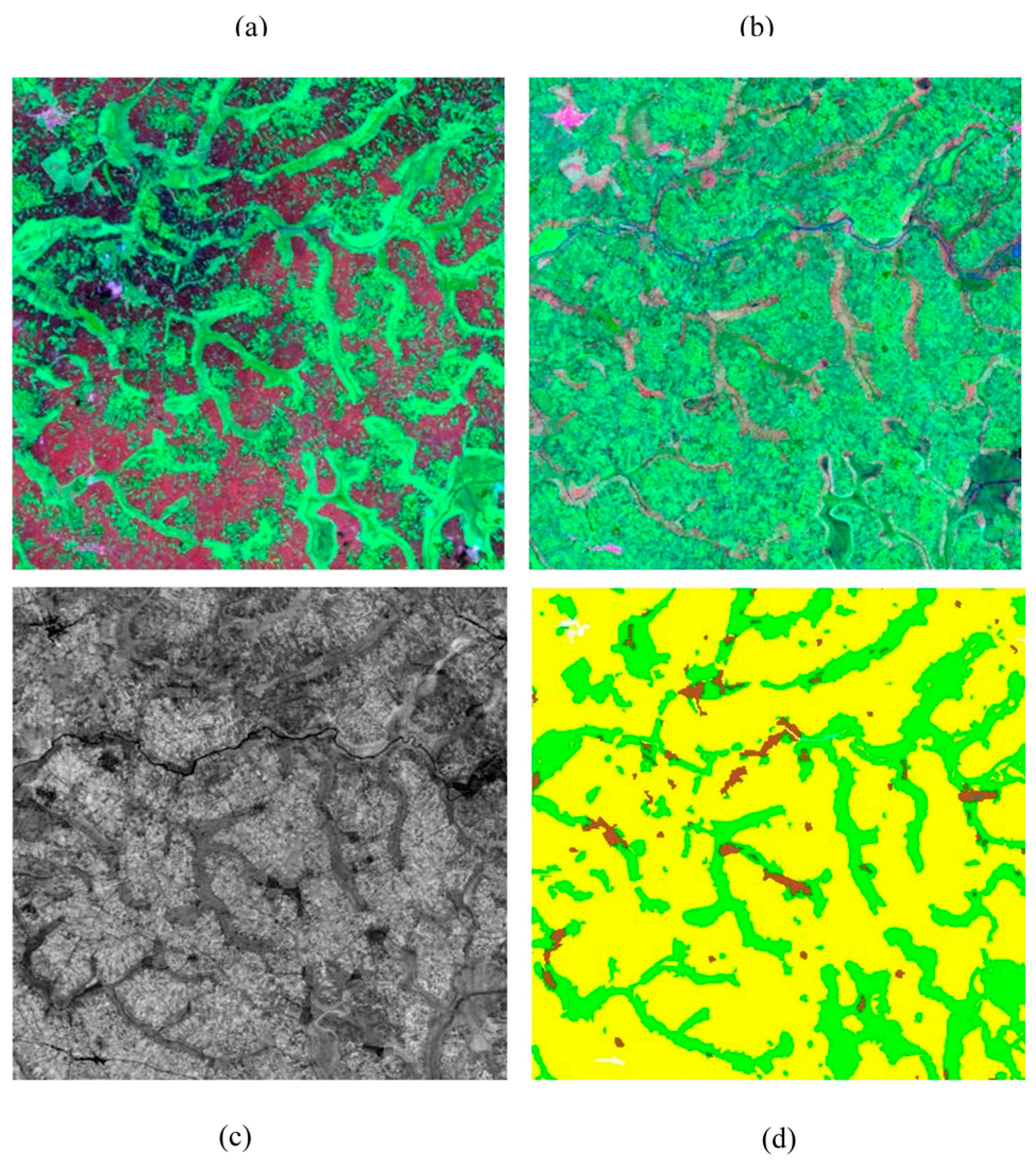
There is more tree and woody cover, as expected, in the west as well as in the gorge of the Abay River. Forests cover about 18% of the study area. The anomalous church forests were well captured in the agricultural highlands. These healthy stands of trees are seen throughout the final map as islands of woodlands within a sea of agriculture.
Figure 4 shows some examples. Finally, almost 11% of the area is grasslands, which includes managed pasture of the highlands and grassy savannah at lower elevations.
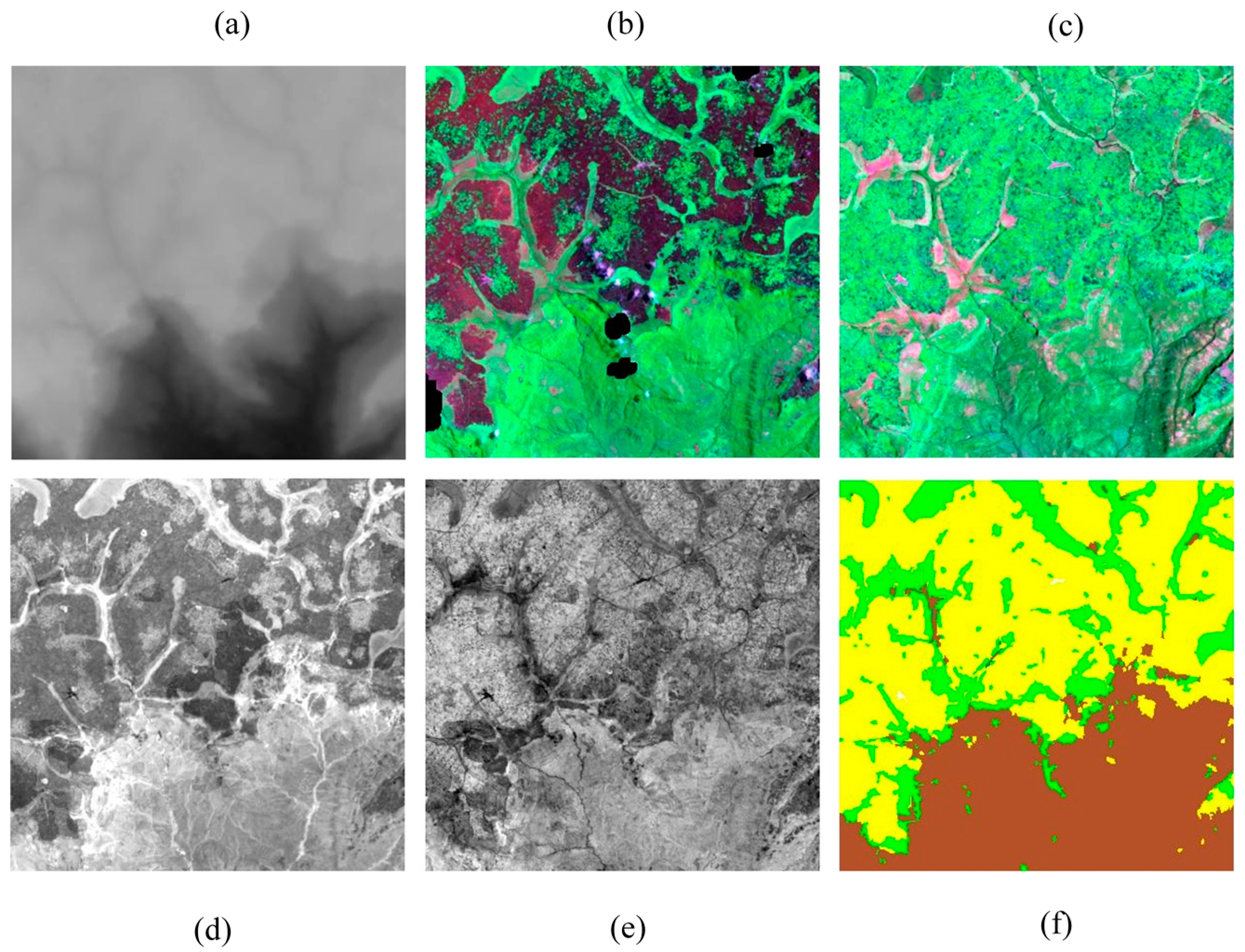
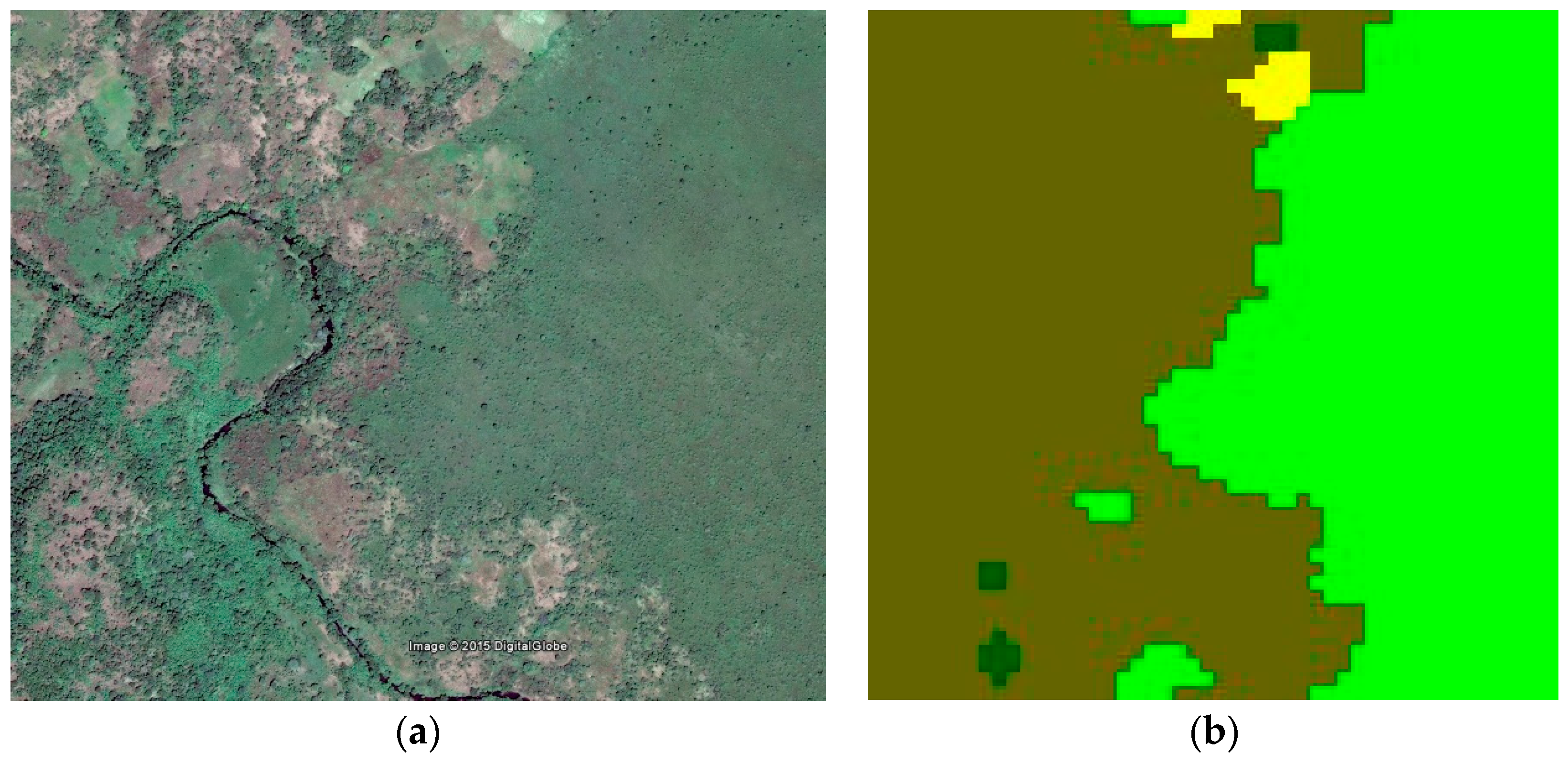
Figure 3 also illustrates the utility of the DEM and the use of temporal mean and variance in NDVI for separating agricultural areas and grasslands from the woody-shrub covered hillsides. The DEM in the upper left panel (a) shows the flatter plateau approach of the mountainside, which falls away quickly. The next two panels show green vegetation differences at two times of the year. The woody shrub maintains some relative greenness in both, whereas the vegetation on the plateau has more pronounced seasonality. The image in the bottom left (d) is the mean of NDVI at each pixel over time. The woody vegetation remains the greenest in terms of mean followed by agriculture and grasslands categories, which are comparable. The next image, variance of NDVI, is most useful for separating the agricultural lands from the grasslands.
Figure 4 also illustrates the utility of using the variance of NDVI over time to separate agriculture and grasslands. The agriculture category has much larger variance than the grassland category. These patterns are then reflected in the final map on the bottom right (f). None of these data layers are likely to have been sufficient to separate these classes had they not been combined with the others. There is significant overlap of classes among these rules and patterns, but the ability of the SVM to work with and combine these different sources of information made the final map possible.
Degraded lands are symptomatic of erosion and overgrazing in these highlands. Areas of both farmland and pasture that have been degraded have been captured in the bare ground class.
Figure 5 shows examples of imagery where farmland and pasture give way to bare ground, shown in white, and its derived classification.
Three of the classes in this map can be found across a continuum of savannah landscapes. In our system, forest gives way to wooded savannah as the canopy opens up, which in turn should be classified as grassland at less than 30% cover. These savannah transitions from woodier savannah to grasslands are a challenge to classify since by definition these are mixed pixels.
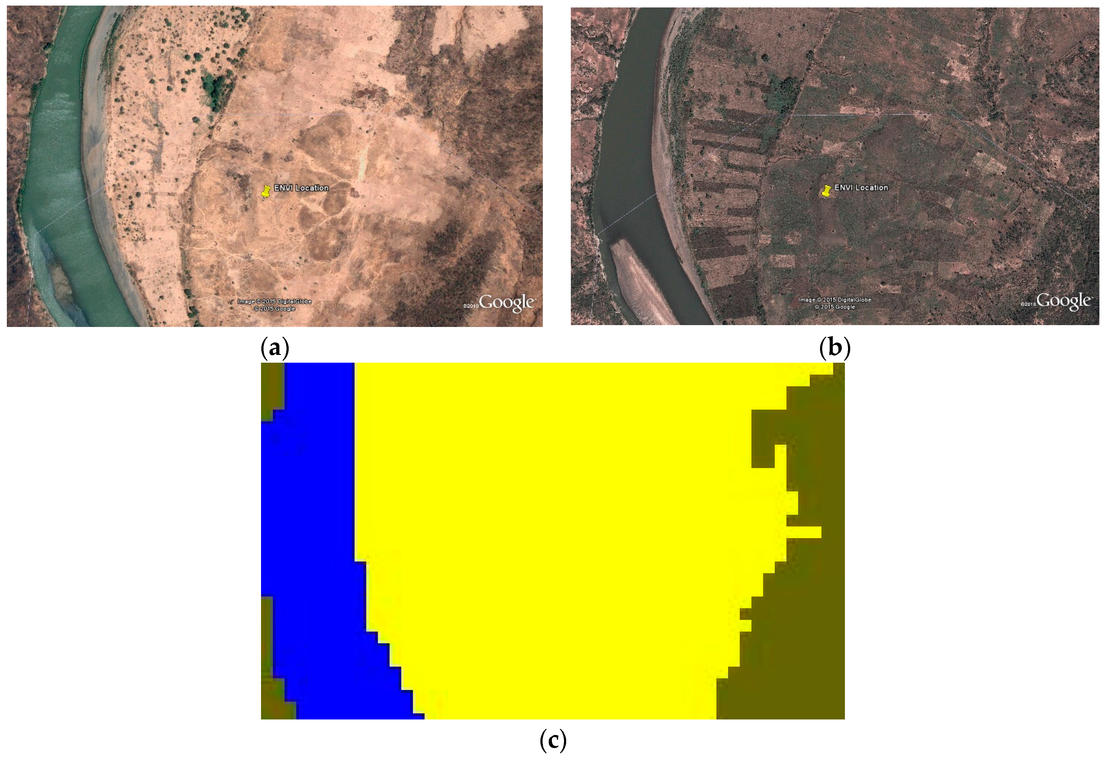
Descending into the gorge of the Blue Nile, dryer conditions prevail. Vegetation is shrubby to barren.
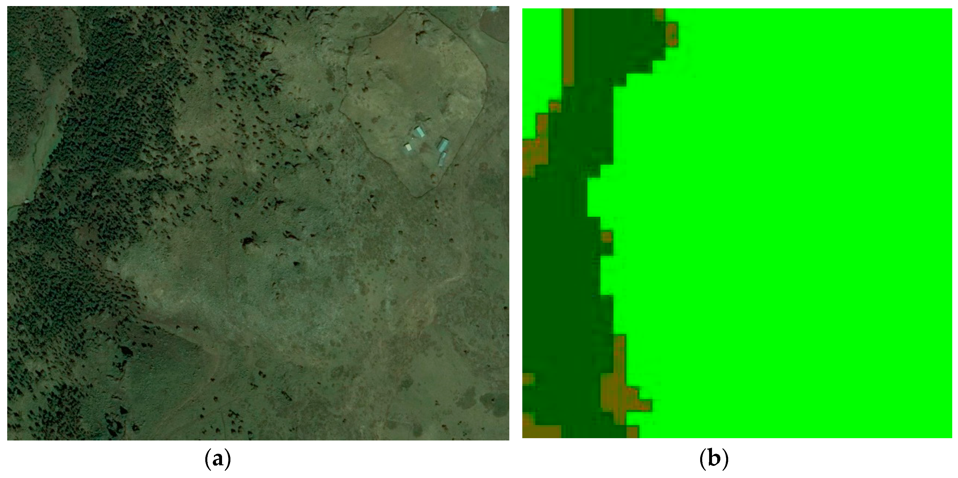
Figure 6 is imagery from above the Abay gorge from different years. In 2004, during the dry season in March, it is difficult to discern any agriculture even though a couple of homesteads are visible. In more recent imagery in December 2011, late in the growing season, it is possible to see some small fields traced within the thorny scrub. The classifier has labeled these as agriculture and wooded/shrub. This is emblematic of some of the most difficult areas to classify in the study area because the low productivity agriculture can be difficult to separate from bare ground with sparse shrub cover. Also notice that it is likely that agriculture expanded toward the river in the upper left of the newer image. This illustrates how change is necessarily masked using the greater temporal depth of imagery, but the full extent of contemporary agriculture is captured.
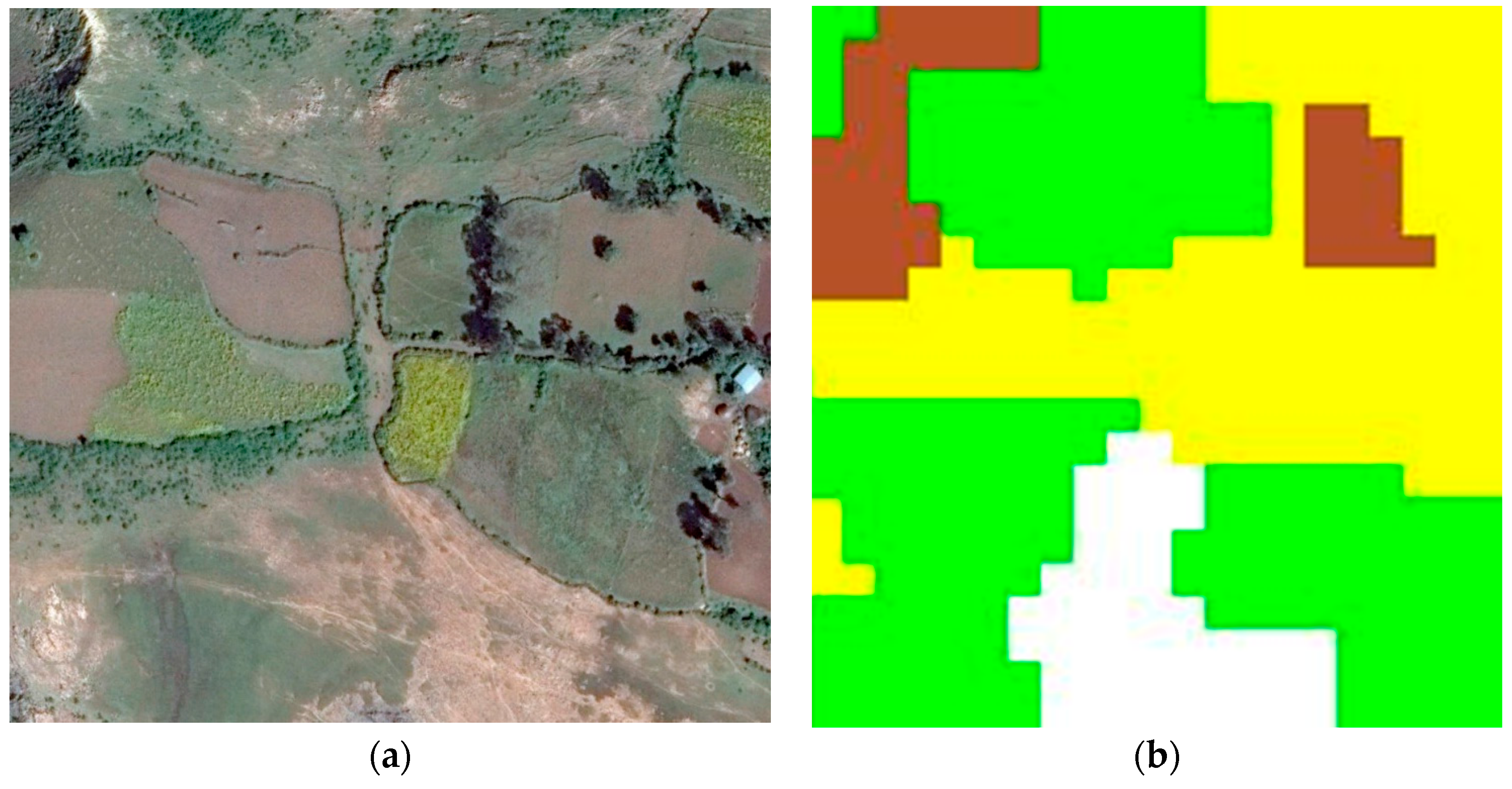
Figure 7 is taken in the lowland savannah of the western frontier and illustrates how the classifier managed separation of woodland savannah and grassland savannah. The grassy right side of the image is dotted with some trees and shrubs but is still open. The left side has more tree cover and some small stands where the canopy may be closed, but most of it still falls below 30% closure although there is substantial variability across a continuum of tree cover. The final classification expresses the major distinctions of grasslands to the right and wooded area to the left, with a small patch of forest at the bottom and a bit of agriculture at the top.
Figure 8 shows part of the peak of Choke Mountain at a point over 3600 masl, which receives greater than 1 m of rainfall per year and is characterized by herbaceous groundcover and some dense stands of trees [
23]. Despite very few cloud-free observations at this peak, the classifier has captured and separated this grassy cover from the forest.
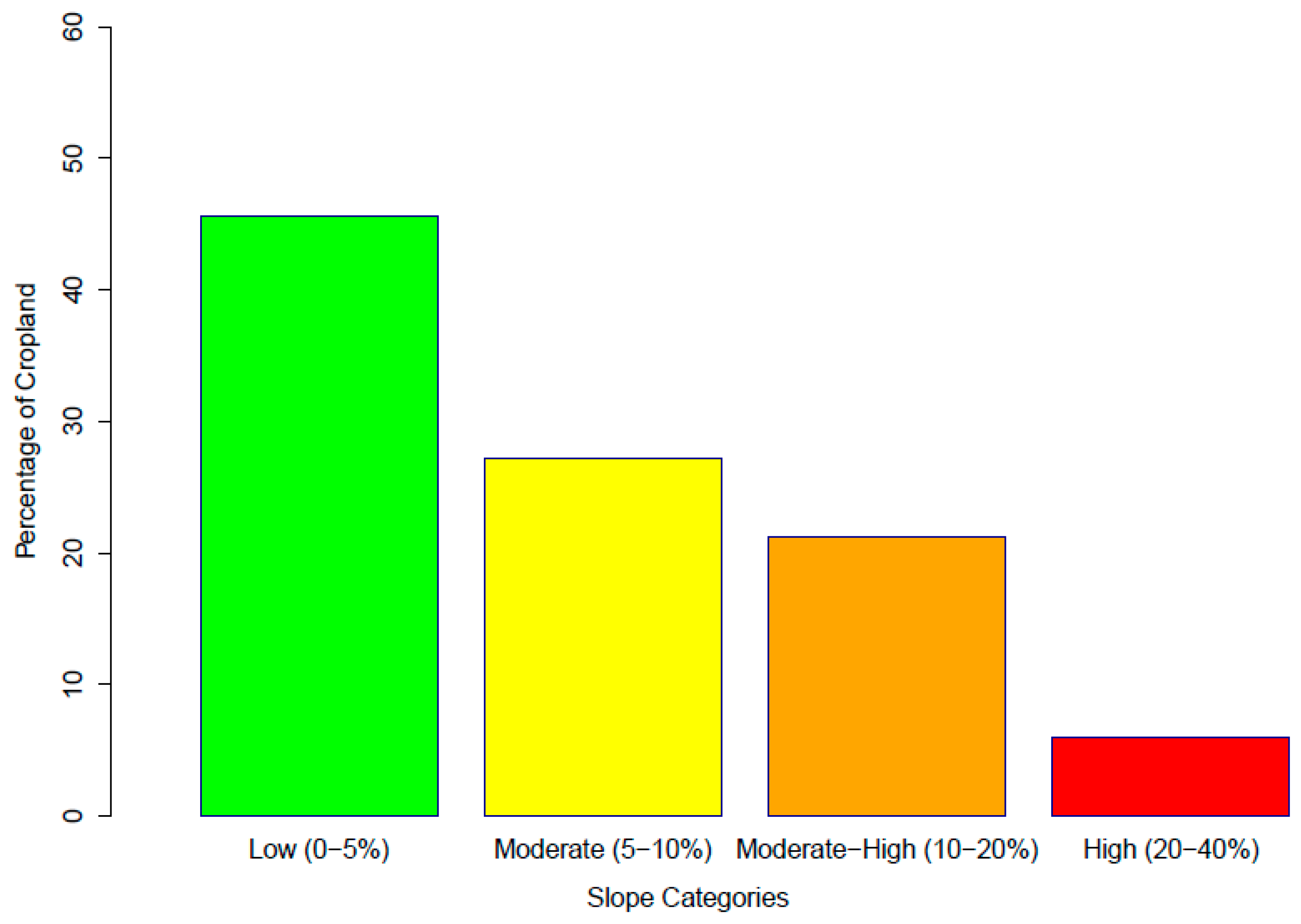
Figure 9 shows how this agricultural area is separated across some broad slope categories. The largest category of agricultural land is found where the slope is less than 5%: this totals about 45%, or more than 3 million hectares. The two middle categories, where slopes increase from 5% to 20%, combine to hold slightly more farmland than the first category. About 3.2 million hectares of agriculture, 200,000 more than with 5% slope, are found in these two categories. Finally, there is significant land with slope greater than 20% that is farmed. This is over 5% or about 400,000 hectares. Omitted from this figure is about 0.1% of agricultural land that was classified on slopes from 40% to 75%. It would hardly register on this graph but would probably include a higher percentage of error of land cover classification and slope calculation.
Table 3 shows the confusion matrix that provides an assessment of the map’s accuracy using the first sampling approach. Overall accuracy is around 55% with average producer’s accuracy at 64% and average user’s accuracy at 55%. Within the most common classes in the study and classes of particular interest in erosion studies (agriculture, wooded, grassland, bare and forest categories), the results were mixed. The agriculture category had producer’s accuracy of 51% and user’s accuracy of 85%. The high user’s accuracy for the agriculture class means that a map user can have 85% confidence that a segment labeled as agriculture is indeed agriculture. The lower producer’s accuracy means the model significantly underpredicted agriculture. It often classified agricultural land as grassland (35 segments), bare (34 segments), wooded (34 segments) and even urban (24 segments) and forest (15 segments). Wooded is the second most common land cover in the map after agriculture and the final results were mixed, with producer’s accuracy of 36% and user’s accuracy of 64%. The classifier most often mislabeled woodlands as forest (53 segments) or marsh (62 segments). Grasslands proved difficult to classify, with 59% user’s accuracy and 52% for producers. The grassland category was significantly mislabeled by the classifier as belonging to all the classes except forest and agriculture, yet the predicted grassland segments on the final map included significant amounts of agriculture (35 segments) and wooded areas (29 segments). The bare ground category had around 54% user’s accuracy and 48% producer’s accuracy and was usually mislabeled as urban (64 segments) or labeled bare when it was actually agriculture (34 segments). Of these more common land cover types, forest had the highest producer’s accuracy at 78%. Its user’s accuracy was just 59%, however, due to confusion with wooded segments.
The results of the second accuracy assessment involving only the cropland category revealed that this category had an overall accuracy of over 76% with a tolerable amount of commission errors but a significant amount of omission error (about 43%) in the non-cultivated category (
Table 4). Of the roughly 3800 samples used in this evaluation, 55% were selected from the cultivated category, and the remainder were selected from the non-cultivated category, encompassing all other categories targeted in this study. Of the roughly 1700 non-cultivated samples selected, grasslands (23%), wooded (48%) and forest (28%) made up the majority of the non-cultivated class. As depicted in
Table 4, the majority of the errors in the cultivated vs. non-cultivated comparison were omission in the non-cultivated category in nature, meaning that many areas that were labeled as non-cultivated in the map should have been mapped as cultivated. To this end, the grasslands category made the largest contribution to the omission error observed in
Table 4—over 77% of the samples labeled as non-cultivated (grasslands) should have been mapped as cultivated. This was followed by the bare ground category where roughly half of the samples were incorrectly classified as that class and should have been mapped as cultivated. The smallest omission error with a significant amount of samples occurred in the forest category—less than 30% of all non-cultivated (forest) samples were incorrectly classified as non-cultivated and belonged to the cultivated category in reality. These results suggest that the main source of confusion in the cropland category was the grasslands—not a very surprising result given the ecology and the topographic position of this land cover type.
4. Discussion
The results of the classification for this difficult mountainous and variable terrain are encouraging. Many aspects of the method performed well and merit consideration when confronted with similar classification problems. The main problems addressed by our study were these:
4.1. Mountainous Terrain
Mountainous terrain is difficult to classify due to cloud cover and topographically-linked variability of land cover classes of interest. First, mountains are often shrouded with clouds, which makes it difficult to measure spectral reflectance from space-based platforms. To deal with the cloud cover, we combined data from several years. This allowed us to obtain a variety of data from the wet and growing seasons, which was integral to discerning phenological differences among our classes. Unfortunately, it necessarily occludes land cover change that must occur over this timeframe, and must also then give rise to some of the error in the classification. Because the classification was driven in part by the need for better erosion studies and crop modeling simulations, the motivation to get the agriculture category correct outweighs some of the error derived from landscape change, and this goal was accomplished since agriculture was mapped at 85% user’s accuracy. The temporal and phenological differences captured in our time stacks was key to separating agriculture from woodlands and grasslands, so this sacrifice was necessary.
The second difficulty in classifying mountainous terrain is that the topography gives rise to variation across the broadly defined classes that interested us. Alpine grasslands at the top of Choke look much different than semi-arid grasslands in the canyon below. More than 10 crops are grown on small plots across various areas of the highlands. The use of the DEM and slope data can effectively turn these differences into an advantage. The SVM classifier can learn that a given class may have a range of expressions across different parts of a mountain. Other classification algorithms might have required that we create more specific sub-class labels in different mountain ecologies and then combine the results into a single class. That would likely create more work in training the classifier and processing the results, so in this case, the use of DEM information with the SVM classifier was a success.
4.2. Diversity of Management and Land Use History
Agriculture in the highlands is practiced on plots of small size using several different crops, each with its own cropping calendar. This creates much variation within and among agricultural pixels in space and time. Farmers planting different crops adjacent to one another in a given year may have planting and harvest dates that differ by months. Over the years that imagery was gathered, various crop rotations may be prevalent in different areas. Again, the SVM can handle this variability, but only if given appropriate and sufficient training data. With a deeper temporal set of data, the onus is on the collector of the training data to find points with unique temporal characteristics as well as unique spatial characteristics. In practice, this entails being mindful of gathering training data that use imagery from a variety of dates and seasons across the breadth of time covered by the satellite imagery selected. The use of a single set of temporal imagery simply because it shows agriculture particularly well would bias the training data toward specific cropping and management practices and miss the fuller expression and extent of agriculture in the study area. The algorithm is always only as good as the data it is given, and in this instance the use of so much input data implies significant effort in data collection and analysis.
4.3. Lack of Reference Data
Research for this project included time spent in the study area on Choke Mountain completing socio-economic survey, but not gathering organized groundtruth data. This fieldwork was still useful for interpreting imagery and training the classifier, but formally collecting validation samples in a structured manner would have been a huge undertaking, given the large and diverse study area and the difficulty of travel in some parts. For this reason, Google Earth high resolution imagery was leveraged for training the SVM algorithm. In some areas, these images are not of sufficient quality to inspire confidence using them in training or accuracy assessment. Often, these areas are the more remote western lowlands and there is better coverage in more populated highland areas. Unfortunately, the remote areas can be among the hardest to classify. Shrubby vegetation makes it impossible to differentiate between grassland and wooded savannah. There are areas of small villages with agriculture that can be confused with grasslands, woodlands and even barren lands if the land is very marginal. The bias in image availability, unfortunately, coincides with this research team’s expertise, which is also concentrated in agricultural communities of the more populated highlands. These biases have certainly affected the results, with agriculture being more successful as a class than the land covers present in the west.
There is also a lack of multi-temporal imagery in the Google high resolution data archives. Often, a single image is not sufficient to determine the class label in this study area, especially if it is a dry season image. Thus, the results are influenced by the season of the imagery available in Google. Where Google Earth has more wet season images, less bare ground may be chosen and vice versa. This can lead to misclassification both in training and in verification. However, this can be minimized if the analyst uses a large number of dates of satellite imagery that are independent of the Google Earth images.
4.4. Explaining Confusion
These challenges in combination caused a certain degree of error and confusion by the classifier. We believe the method of combining multitemporal imagery and DEM derived information with a nonparametric pattern recognition algorithm was more successful than a classification that used a single year of imagery could have been. However, the method was still hindered even by these challenges it was meant to address.
Agriculture covers a large proportion of these highlands. When the classifier identified a piece of land as agriculture, it was correct most of the time, probably because the chances favored that it was. Unfortunately, many other segments of agriculture were labeled erroneously, such as grasslands, bare, or wooded lands. Pixels and segments mixed with these land cover types and some land cover change over time are likely the reason for this deficiency. Over the landscape, these categories often occur together and morph among one another over time. There is no regular fallowing in many of the core agricultural areas, but even intermittent fallowing and cycling of marginal lands into or out of production on the edges would cause difficulty for the classifier, depending on when it was able to get clear observations of a specific location in the timestack.
Grasslands, similarly, proved difficult to classify for these reasons and possibly due to the variety of its expression. Even within a single Landsat scene, grasslands vary due to a wide rainfall gradient or human impacts and management. In a very small area, grasslands may be lush, managed pasture, degraded former farmland, or less shrubby hillside. In training, all these were gathered into the single class “grasslands” with no awareness of how the training sample might be skewed to one or another of these types. Certainly, the higher productivity, managed pastureland would be over-represented because it was easily identified in the images in the 7-4-2 Landsat TM band combination during the dry season through to early in the cropping season (~January–July). This tendency was remedied through an iterative approach to training data collection and classification. When the analyst saw errors relative to types of a certain land cover class, more training data would be gathered for that subtype. It would have been more efficient to collect training data by explicitly splitting the land cover into these subtypes during training and classification so that the number of training pixels in each could be readily seen. Then, the subtypes could have been rolled into the single, overarching type when making the final map.
4.5. Assessing Agriculture on Slopes
One of the goals of this study is to support future soil erosion, soil mapping, and crop modeling studies by mapping the patterns of land use and land cover at the scale of smallholder use. The high user’s accuracy in the agricultural landcover map will prove useful in any such research. Although agriculture is still somewhat underestimated in this map, areas which are labeled as agriculture are likely to be agriculture with a high degree of confidence. The study thus provides important new assessment of where agriculture is being practiced in the Abay basin and this information is crucial for spatially-explicit studies of erosion or crop modeling.
Cultivation of sloping farmland in this area does not, in and of itself, automatically imply land degradation, as there are numerous soil conservation practices employed in highland agricultural systems. At the spatial resolution of the DEM and slope layers, for instance, it would be impossible to account for terraces on hillsides, which could be in the order of ten meters wide.
Figure 9, however, does provide a window into some challenges for soil conservation in the study area. On the positive side, more than 45% of the land labeled agriculture in the final map was in a low slope category (<5%). There are also more than 400,000 hectares of farmland with slope over 20%, the legal limit on which land may be cultivated. Further, almost 1.5 million hectares of agricultural land were located on slopes of 10%–20%.
Errors are also likely in slope calculations, beginning with potential discrepancies in the elevation measurements of the DEM. The size of the window used in computing slope can change the result of slope analysis significantly and exacerbate or dampen the propagation of the DEM error [
46]. A 5 × 5 pixel moving window used here was judged to be superior to a 3 × 3 pixel window calculation over the same DEM dataset as it appeared smoother and with less noise. Increasing window size further would have reduced error, but at the cost of excessive generalization [
46]. Taken as a whole, the slope data derived from the 5 × 5 window was a compromise that would generally smooth areas of higher slope but still provide reliable information for the point in question without overgeneralizing. Since the agricultural land is also acknowledged to be an underestimate of total agricultural lands, it follows that the slope analysis of agricultural land is also conservative. This provides a useful lower limit to characterizations of where and how much sloping land may be cultivated in the study area. However, we again caution that soil conservation techniques are unaccounted for in both the land cover map and the slope map and obviously would need to be incorporated in any soil erosion study. The authors have commonly observed bunding, hedging and terracing, among other techniques, on many hillside agricultural lands in the study area. The authors have also observed their absence, especially on some steeper slopes, which may be under cultivation opportunistically, temporarily or illicitly.
4.6. Comparison with Existing Land Cover Products
The reported overall accuracy of 55% here compares well with the 48% accuracy in Ethiopia in FROM-GLC [
11]. Improved FROM-GLC did not report accuracy per country but does report accuracies per class [
12]. Its Random Forest classification performed best and comparison of its user and producer’s accuracies for similar class labels is given in
Table 5. Generally, the map presented here does well compared to the Improved FROM-GLC especially given the difficulty the FROM-GLC product experienced with Ethiopia. In the agriculture class, our map does generally as well, but better if looking at the high confidence samples of
Table 4. Our map shows an improvement in the difficult Grassland and Shrub categories. Our map falls short of the standard of Improved FROM-GLC in Forest, Water and Bare Ground, but these classes are a small fraction of total mapped area of the Ethiopia map when compared with the area Agriculture, Grassland and Wooded/Shrub. This supports our claim in the utility of our product for environmental assessment of this region of Ethiopia.
5. Conclusions
This challenging land cover classification is judged a mixed success. It has advanced knowledge of land cover of a difficult to map area for which global and regional scale maps had struggled. Agriculture is mapped with high accuracy, and the map captured important patterns of cropland, grassland, and shrubland in the highlands. For applications such as erosion studies and crop modeling, it is a significant step forward, since this productive landscape is mapped accurately at a scale commensurate with smallholder land use patterns for the first time in such a large area of Ethiopia. Some important classes in the map do have low producer’s and consumer’s accuracies and effort needs to be made to improve these with better reference data. The western part of this study area is more dynamic with extensive production systems and, likely, significant conversion of savannah to intensive agriculture in the last 10 years, and will need focused attention and mapping in that regard in the future. With the addition of better imagery and validation data, the methods used in making this map will also work for the western edge of the study area, so again, progress can be counted even on this western frontier.
Going forward, researchers should do three things. (1) Apply similar methodology to other difficult mapping areas that have not been well captured by global scale maps at this type of resolution; (2) Use this map in environmental applications in the study area; (3) Improve this map on the western lowland side since it is an area of ongoing landscape change.


