Article

Comparison of Tree Species Classifications at the Individual Tree Level by Combining ALS Data and RGB Images Using Different Algorithms

1
Institute of Mountain Science, Shinshu University, Nagano 399-4598, Japan
2
Finnish Geospatial Research Institute, Geodeetinrinne 2, 02430 Masala, Finland
3
Key Laboratory of Forest Ecology and Management, Institute of Applied Ecology, Chinese Academy of Sciences, Shenyang 110016, China
*
Author to whom correspondence should be addressed.
Remote Sens. 2016, 8(12), 1034; https://doi.org/10.3390/rs8121034
Submission received: 19 September 2016 / Revised: 12 December 2016 / Accepted: 14 December 2016 / Published: 19 December 2016

Abstract

:
Individual tree delineation using remotely sensed data plays a very important role in precision forestry because it can provide detailed forest information on a large scale, which is required by forest managers. This study aimed to evaluate the utility of airborne laser scanning (ALS) data for individual tree detection and species classification in Japanese coniferous forests with a high canopy density. Tree crowns in the study area were first delineated by the individual tree detection approach using a canopy height model (CHM) derived from the ALS data. Then, the detected tree crowns were classified into four classes—Pinus densiflora, Chamaecyparis obtusa, Larix kaempferi, and broadleaved trees—using a tree crown-based classification approach with different combinations of 23 features derived from the ALS data and true-color (red-green-blue—RGB) orthoimages. To determine the best combination of features for species classification, several loops were performed using a forward iteration method. Additionally, several classification algorithms were compared in the present study. The results of this study indicate that the combination of the RGB images with laser intensity, convex hull area, convex hull point volume, shape index, crown area, and crown height features produced the highest classification accuracy of 90.8% with the use of the quadratic support vector machines (QSVM) classifier. Compared to only using the spectral characteristics of the orthophotos, the overall accuracy was improved by 14.1%, 9.4%, and 8.8% with the best combination of features when using the QSVM, neural network (NN), and random forest (RF) approaches, respectively. In terms of different classification algorithms, the findings of our study recommend the QSVM approach rather than NNs and RFs to classify the tree species in the study area. However, these classification approaches should be further tested in other forests using different data. This study demonstrates that the synergy of the ALS data and RGB images could be a promising approach to improve species classifications.

Graphical Abstract

1. Introduction

The planted forests in Japan cover approximately 10 million ha [1]. Although harvest activities have almost stopped in some forests because of decreases in timber prices during the past 30 years, recently, many forest owners have had to improve their harvest efficiency to deal with the foreign competition related to the Trans-Pacific Partnership (TPP) agreement. One solution for the improvement of timber productivity is obtaining accurate and timely information on the condition of forest resources to support decision making. In addition, most privately owned forests, which account for approximately 58% of the total forested area in Japan [1], were entrusted to FOCs (Forest Owners’ Cooperatives) for management with the main purpose of wood production. To date, forest information, such as species composition, diameter at breast height (DBH) and stem density, has been obtained from traditional field-based surveys. The FOCs are eager to obtain spatially explicit and up-to-date stand information on DBH, tree height, volume and species distribution patterns over large areas at a low cost. More than 50% of Japanese land has been covered by airborne laser scanning (ALS) as of July 2013 [2]. The FOCs can obtain ALS data at a low cost, but they do not possess techniques to interpret the data. Consequently, the forest industry in Japan is looking to the next generation of forest inventory techniques to improve the current wood procurement practices.
Remote sensing has been established as one of the primary tools for large-scale analysis of forest ecosystems [3]. It has become possible to measure forest resources at the individual tree level using high resolution images and computer technology [4,5]. However, it is nearly impossible to estimate the DBH and volume attributes of forests at the single tree level using only two-dimensional airborne and satellite imagery [6,7]. One of the most prominent remote sensing tools used in forest studies is ALS, which measures distances by precisely timing a laser pulse emitted from a sensor and reflected from a target, resulting in accurate three-dimensional (3D) coordinates for the objects [8]. With the capability of directly measuring forest structure (including canopy height and crown dimensions), laser scanning is increasingly used for forest inventories at different levels [9]. Previous studies have shown that ALS data can be used to estimate a variety of forest inventory attributes, such as tree height, basal area, volume and biomass [7,10,11,12,13]. Several researchers have developed area-based approaches to estimate forest attributes at the stand level using ALS data [14,15,16]. However, few studies have focused on the automated delineation of single trees in Japanese forests [17].
Precision forestry, which can be defined as a method to accurately determine the characteristics of forests and treatments at the stand, plot or single tree level [18], is a new direction for better forest management. Individual tree detection technology plays a very important role in precision forestry because it can provide precise forest information required at the above three levels. Individual tree-level assessments can also be used for simulation and optimization models of forest management decision support systems [18]. During the past two decades, many approaches have been developed to detect individual tree crowns from remotely sensed data [10,19,20]. Early studies focused on assessing individual trees based on optical imagery with high resolution [21,22,23]. With the wide introduction of ALS into remote sensing, an increasing number of studies have undertaken individual tree detection using point clouds [12,24,25]. Through time, these studies have shown increased complexity of analyses, increased accuracy of results, and a focus on the use of ALS data alone [26,27]. Lu et al. [28] provided a literature review of more than 20 existing algorithms for individual tree detection and tree crown delineation from ALS, which showed overall accuracies ranging from 42% to 96% depending on the point density, forest complexity and reference data used. In general, these developed algorithms can be divided into two types: one uses a rasterized canopy height model (CHM) to delineate tree crowns [25,29,30], and the other directly uses 3D point clouds to detect individual trees [12,31,32]. Considering the effectiveness of the different tree crown delineation methods, some comparative studies were recently published showing that, depending on the forest type and structure, one method can be superior to another [33,34,35]. For example, the CHM-based approaches, such as inverse watershed segmentation and region growing algorithms, work best for coniferous trees in boreal forests [24,36,37]. The 3D point-based approaches sometimes successfully identify suppressed and understory trees [12,
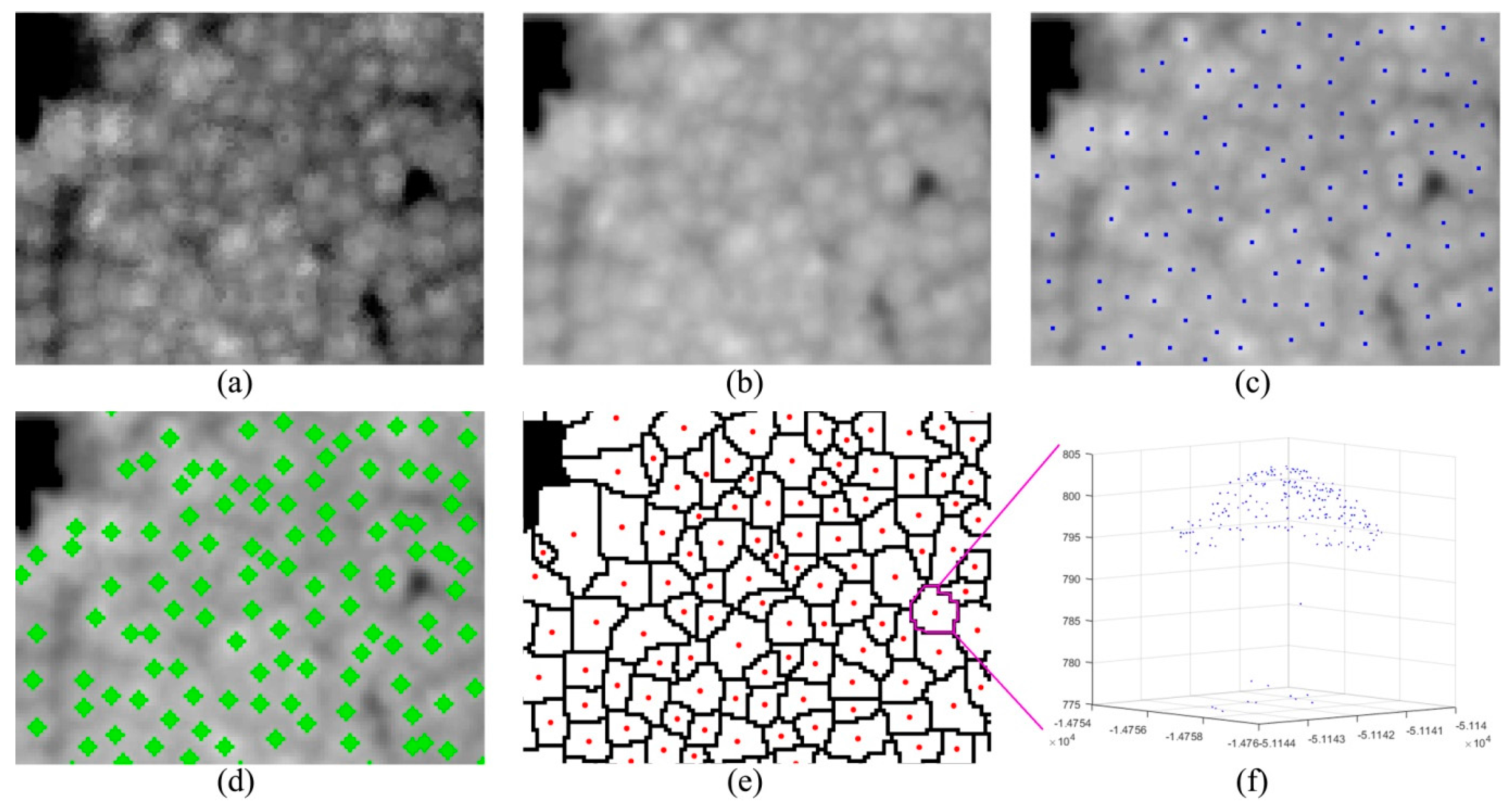
38], while most of the algorithms have lower accuracies over more structurally complex forests, especially in highly dense stands with interlocked tree crowns. Overall, single tree delineation in dense temperate and subtropical forests remains a challenging task. A marker-controlled watershed segmentation has shown a powerful capability for individual tree delineation in numerous previous studies [9,25,39,40].
Conventional existing methods for classifying forest species from remotely sensed data are mostly based on the spectral information from forest canopies [5,41]. Despite vegetation cover classification successes at the stand and landscape levels [42,43], improved accuracy of species classification at the individual tree level is still needed [4]. The availability of laser instruments to measure the 3D positions of tree elements, such as foliage and branches, provides an opportunity to significantly improve forest species classification accuracy [44]. During the last decade, a large number of researchers have contributed to the study of tree species classification using ALS data [45,46,47]. Several ALS features have been extracted to describe crown structural properties of individual trees, such as crown shape and vertical foliage distribution [44,48]. These features are usually calculated based on the parameters of a 3D surface model fitted to the ALS points within a given tree [38,45,49]. However, most of the previous studies showed that it is difficult to accurately classify mixed forests based solely on point clouds [30,46,50,51,52]. Consequently, the combinations of ALS points with passive data sources, such as multispectral and hyperspectral images, have also been used to classify tree species at the single tree level [27,53], but most studies focused on test sites located in boreal forests with a relatively simple forest structure [40]. However, species classification at the single tree level in Japanese temperate forests remains a challenging task. Stand density is generally higher, deciduous tree crowns are often interlocked, and species mixture is greater and more irregular compared with other temperate forests.
Selection of classification approaches plays an important role in forest species identification. Traditional parametric classification methods, e.g., Maximum Likelihood (ML), are easily affected by the “Hughes Phenomenon,” which arises in high dimensionality data when the training dataset size is not large enough to adequately estimate the covariance matrices [53]. In forest classification studies, acquiring a sufficient amount of training data that exceeds the total number of spectral bands and other features required for the ML classifier is an impractical task, especially in highly spectrally variable environments. Consequently, non-parametric machine learning methods such as decision tree approaches have recently received increasing attention in species classification studies [54]. The most commonly used approach is support vector machines [27,39,40,47,48,55,56]. Random forest classification [57] is considered as a solution to overcome the over-fitting issue [50,53,58,59]. Additionally, some researchers believed that linear and quadratic discriminant analysis classifiers were more suitable for their studies [44,51,60]. To the best of our knowledge, only a few studies compared the performance of different approaches in forest classification. For example, Li et al. [61] investigated three machine learning approaches—decision trees, random forest, and support vector machines—to classify local forest communities at the Huntington Wildlife Forest located in the central Adirondack Mountains of New York State and found that random forest and support vector machines produced higher classification accuracies than decision trees. However, assessing the performance of different methods in tree species identification at the individual tree level is still needed. Based on the above analyses, this study focused on the following objectives:
  • To assess the utility of ALS data for measuring single tree crowns in Japanese conifer plantations with a high canopy density using the watershed algorithm;
  • To determine the best combination of spectral bands and structural features for tree species classification; and
  • To evaluate the capability of different machine learning approaches for forest classification at the individual tree level.

2. Materials and Methods

2.1. Study Area and Field Measurements

The study area, located in Nagano, central Japan, is part of the campus forests of Shinshu University. The center of the test site is located at 35°52′N, 137°56′E and has an elevation of 770 m above sea level. The area belongs to the temperate zone and consists of high-density plantations with coniferous trees ranging from 30 to 90 years old. In this study, compartments 1–7 of the campus forests, with an area of approximately 7.3 ha, were selected as the research object (Figure 1). The forests in the study area are mainly dominated by Pinus densiflora (Pd), Chamaecyparis obtusa (Co), Larix kaempferi (Lk), and secondary broadleaved trees (Bl).
Field measurements were undertaken from April 2005 to June 2007. All trees with a DBH larger than 5 cm were tallied, and the species, DBH and tree height were recorded. Each tree was tagged with a permanent label and noted as either live or dead, and the DBHs were measured to the nearest 0.1 cm. Tree locations were calculated using the geographic coordinates of the vertices of the plots and were mapped to the nearest 0.1 m. The plot vertices were measured with a Global Positioning System (GPS) device (Garmin MAP 62SJ, Taiwan), and the locations were post-processed with local base station and orthoimages, resulting in an average error of 0.465 m (RMSE: 1.87 pixels with a resolution of 25 cm). The descriptive statistics of the forests in the seven compartments are summarized in Table 1. The DBH frequency distribution of all trees in the study area is shown in Figure 2. In addition, the forests in compartments 4 and 2 were investigated again in June 2015 and June 2016, respectively, to determine whether the dominant tree species in the canopy layer had changed. The results suggested no obvious changes in the canopy layer because no timber harvesting activities were conducted during this period.

2.2. Airborne Laser Data and True-Color (Red-Green-Blue—RGB) Images

Airborne laser scanning data were collected in June 2013 using a Leica ALS70-HP system (Leica Geosystems AG, Heerbrugg, Switzerland). The system was configured to record up to three echoes per pulse, i.e., first or only, intermediate and last. The wavelength of the laser scanner is 1064 nm. In this study, the point cloud data were acquired at a flight altitude of approximately 1800 m above ground level and at a speed of 203 km/h. The scanner was operated at a pulse rate of 308 kHz (i.e., 308,000 points per second), with a maximum scanning angle of ±15° and a beam divergence of 0.2 mrad. The specifications rendered the density of the collected point clouds to be at least 4 points per m2. To obtain a high point density, each flight line was surveyed twice using the laser scanner to provide 50% overlapping strips, which allowed us to acquire a point density ranging from 13 to 30 points per m2 (over the forested area). In addition, true-color (RGB) images with three bands (red, green and blue) and a resolution of 25 cm were acquired at the same time as the laser data from the RCD30 sensor using the color mode.

2.3. Data Analyses

The research flow chart in Figure 3 provides an overview of the methods.

2.3.1. Establishment of Canopy Height Model (CHM) and RGB Orthoimages

CHM and RGB orthoimages were created using the following steps: First, ground points were automatically extracted from the original point clouds using the standard approach in TerraScan software. Second, the ground points were manually corrected, and a digital elevation model (DEM) with a resolution of 50 cm was generated using the corrected ground points based on the TIN (triangulated irregular network) algorithm. Next, ortho-rectified RGB images were created using the above DEM data and raw camera photos in TerraPhoto software. Subsequently, a digital surface model (DSM) with a resolution of 50 cm was generated using the point cloud data, in which the height of the highest point in each grid with a length of 50 cm was considered to be the DSM value of the corresponding pixel. A CHM was then calculated by subtracting the DEM from the DSM. An image registration using polynomial fitting was finally completed for the RGB orthoimages based on the CHM, with an average error of 0.41 m (RMSE: 0.82 pixels). In addition, an intensity map with a 50 cm resolution was generated by averaging the laser intensity values of all points within each pixel.

2.3.2. Correcting for CHM Artifacts

An accurate delineation of tree crowns required generating a CHM with a high resolution of 50 cm [62] such that a ground point did not always occur within each pixel [27]. As a result, the CHM data contained a number of artifacts that prevented the successful segmentation of tree crowns. In particular, the CHM contained many severe elevation drops, especially in the middle of the canopy. The elevation drop artifacts were directly related to the scanning pattern of the laser sensor, i.e., the z-value thin troughs were located between the lines of the laser scans [27]. The challenge was further complicated because the artifact pixels were not NaN (Not a Number) values; rather, their values were well within a typical CHM. This problem has been noted before, especially when attempting to delineate individual trees [62]. Jakubowski et al. [27] presented an effective and detailed method to correct these artifacts in their research. However, this method did not work well for our data in this study. Consequently, we developed a simpler and more feasible approach to mitigate this problem using the following steps: First, the original CHM data (called ORG) were processed using a focal statistics calculation with a circular kernel of 3-pixel radius, which was completed using ArcGIS software, and the result was saved as FOCAL; second, the original CHM was smoothed twice using a low pass filter with a window of 3 × 3 pixels, and the result was saved as FILTER; then, the outlier pixel values in the original CHM were corrected using two conditional calculations: (1) if FILTER − ORG ≥ 1 m, the original pixels of the CHM data were valued as FOCAL; and (2) if FILTER – ORG ≤ −1.5 m, the original pixels were valued as FILTER. A part of the original and corrected CHM data is displayed in Figure 4.

2.3.3. Individual Tree Detection and Feature Extraction

Single tree detection and crown segmentation in the study area were performed using the above corrected CHM data and a marker-controlled watershed algorithm. During the segmentation processes, the tree crown shapes and individual tree locations were determined using the following steps [9,63]. (1) The corrected CHM (Figure 5a) was smoothed with a Gaussian filter to remove small variations on the crown surface. The degree of smoothing was determined by the standard deviation value (Gaussian scale) and kernel size of the filter. A standard deviation of 0.7 and a bandwidth of five pixels were used based on trial and error. The Gaussian smoothed CHM is displayed in Figure 5b; (2) Local maxima (LM) searches were performed in a sliding neighborhood of 5 × 5 pixels. These local maxima were considered as potential tree tops (Figure 5c). Due to the dispersive crown shape of the large deciduous trees, the LM algorithm tended to extract more than one tree top within a tree crown. Consequently, these local maxima were dilated using a dish-shaped structuring element with a radius of two pixels (Figure 5d); (3) The dilated local maxima were then used as markers in the following marker-controlled watershed segmentation for tree crown delineations. Each segment was considered to present a single tree crown, and the highest laser point height within each segment was used as an estimate of the tree height (Figure 5e). In total, 2438 tree crowns were detected in the study area.
After the individual tree crowns were segmented from the CHM, the laser returns that fell within each segment were extracted and used to derive the tree features (Figure 5f). Both structural and spectral features were generated from individual tree point clouds, CHM and RGB orthoimages. As a result, a total of 23 tree-level variables were extracted, consisting of 17 ALS-derived metrics and 6 optical metrics (Table 2). Additionally, the species of all segmented tree crowns in the study area were manually identified based on the field data and other information, including high resolution orthophotos and existing thematic maps.

2.3.4. Crown-Based Supervised Classification and Counting of Different Tree Species

In this study, to overcome the “mixed pixels” problem of the pixel-based classification (i.e., some pixels within a tree crown may be classified into two or more different classes), each tree crown was considered to be an object that was classified using its attributes extracted from the ALS and orthophoto data (Table 2). Seven approaches with 24 algorithms were compared (Table 3). In addition, the 23 tree features were divided into three groups: ALS-derived features (17), spectral orthoimage-derived features (6), and the combination of both data sources (23). The best method and best combination of tree features for species classification were identified using the following steps: (1) The 2438 segmented tree crowns with manually identified species were randomly split into 70% and 30% portions for a training dataset (n = 1707) and a validation independent dataset (n = 731), respectively. The calibration dataset was used to train the prediction models, while the validation dataset was used to test the quality and reliability of the prediction models. (2) The first five methods, including decision trees (DT), discriminant analyses (DA), support vector machines (SVM), K-nearest neighbors (KNN) and ensemble classifiers (EC), with 22 algorithms were trained using 16 and 84 combinations that were randomly selected from the 17 ALS-derived and all 23 features, respectively. This was performed using the classification learner application in Matlab R2015b software [64]. (3) The six RGB image-derived metrics were selected as the basic dataset to determine the best combination of tree features for species classification because these metrics provided an acceptable classification. In detail, these RGB features were first used to classify the tree crowns using the quadratic support vector machines (QSVM) approach; then, each combination of the basic dataset with each ALS-derived feature was used to perform a classification, and the combination that had the highest increment in overall accuracy was selected as the new basic dataset; next, each combination of the new basic dataset with each remaining ALS-derived feature was used to perform a classification, and the combination with the highest increment in overall accuracy was chosen as the new basic dataset; the above process was repeated until the overall accuracy of all of the new combinations decreased in comparison to the previous classification step. (4) The feature combinations that had the highest overall accuracy in each loop process were also used to perform tree crown classifications using the neural network (NN) and random forest (RF) approaches to compare the results obtained using the QSVM approach. The NN and RF classifications were completed using the Neural Network Toolbox in Matlab R2015b [65] and R 3.2.3 software, respectively. The detailed procedure of RF classifications using R software is listed in our previous studies [43,66].
After the tree crown-based supervised classification processes were completed, the total number of trees of different species in each compartment was counted using the summarize function in ArcGIS v10.0. The detected accuracy of the tree crowns can be calculated using the following formula:
φ = (1 − |ND − NF|/NF) × 100
where φ is the delineated accuracy (%), ND is the number of the trees detected by the watershed segmentation method, and NF is the number of the trees in the field data. In this study, based on the DBH frequency distribution of all of the trees in the study area and the average DBH in each compartment (Figure 2, Table 1), the trees with a DBH larger than 25 cm in the field data were selected as the canopy trees and were used to test the accuracy of the delineated tree crowns to distinguish between species.

3. Results

3.1. Comparison of Classification Methods

The 100 trained models were used to classify the validation dataset, and their overall accuracies are summarized in Figure 6. The results indicated that the QSVM approach had a higher overall accuracy compared with the other methods.

3.2. Delineation of Tree Crowns and Identification of Tree Species

As a result, a total of 2438 trees with an average accuracy of 93.54% were detected in the seven compartments (Figure 7). In terms of different compartments, more than 91% of the trees in each compartment were delineated except for compartment 1, which had an accuracy of 71.8%. In compartment 1, 163 upper trees were recorded in the field data, while 209 tree crowns were generated from the CHM data. This is because the forest in compartment 1 was mainly dominated by large broadleaved trees, and those deciduous trees with dispersive crowns were easily split into multiple crown components, which resulted in one segment for each component. In addition, there was a young Larix kaempferi stand in this compartment, which led to a lower count based on the field data compared with the interpreted results. After the tree crowns were detected based on the CHM, the species attributes of each crown were manually identified using field data, multi-temporal airborne images, and existing thematic maps. As a result, the delineated tree crowns and tree tops distinguishing the species are shown in Figure 8 by overlaying the true color image with a transparency of 50%.

3.3. Object-Based Supervised Classification of the Tree Species

3.3.1. Determining the Best Combination of Tree Features for Species Classification

The trained QSVM model using the 1707 tree crowns was used to predict the species attributes of the 731 test tree crowns, and an overall accuracy of 76.7% was obtained with the use of the six RGB features derived from the orthoimagery (Table 4). Then, 17 combinations of the six RGB features with each ALS feature were used to train the QSVM model and to predict the species of the test tree crowns. As a result, the combination of the RGB and LI features had a higher overall accuracy, with a value of 83.3%, in comparison to the other combinations in the first loop. In the second loop, the combination of RGB, LI, and CHA features had the highest overall accuracy of 88.8%, with an improvement of 5.5 percentage points compared to the best result of the previous loop. Until the seventh loop was performed by repeating the above steps, no improvement in the overall accuracy was found in the 11 combinations (Table 4). In addition, the combination of all 23 features was tested in this study. However, the overall accuracy obtained was 87.6% (Table 5). Consequently, the combination of RGB, LI, CHA, CHPV, SI, CA and CH, which was identified in the sixth loop, can be considered the most suitable dataset to classify the tree crowns in the study area.

3.3.2. Comparison of Classifications of the Tree Crowns Using Different Approaches

The datasets from RGB, all 23 features, and the combinations that had the highest overall accuracies in the six loops were used to train the NN and RF models and to predict the species of the test tree crowns. As a result, an accuracy report of the three methods was generated, as shown in Table 5. The results suggest that the overall accuracies of the classifications using the NN approach, with values ranging from 81.6% to 91%, were much higher than those using the RF classifier, with values less than 85%. Additionally, the producer and user accuracies of the different species for the classifications of the tree crowns classified using the three approaches with the highest overall accuracy are summarized in Figure 9. The results indicate that the QSVM and NN approaches resulted in superior classifications compared with the RF method, and QSVM was slightly better than NN. Consequently, the trained models using the QSVM and NN algorithms were used for further analyses.

3.4. Counting Trees of Different Species in the Study Area

All of the detected tree crowns in the study area were classified using the QSVM and NN models developed in Section 3.2. As a result, two classification thematic maps of tree crowns were generated, as displayed in Figure 10, by overlaying the RGB orthoimages with a transparency of 50%. The number of detected tree crowns that distinguished the species in each compartment and in the whole study area was then counted using the spatial statistics function in ArcGIS software, and these results, as well as the count values from the field data, are listed in Table 6. The results suggest that Pinus densiflora and Larix kaempferi were the main dominant species in the forests in compartments 1, 3 and 4. Additionally, the forests in compartments 4 and 1 were co-dominated by Chamaecyparis obtusa and large broadleaved trees, respectively. However, Pinus densiflora was the most dominant species in compartment 2. The canopy trees in compartments 5–7 were mainly dominated by Pinus densiflora and Chamaecyparis obtusa. Although most of the dominant canopy trees in the different compartments were successfully delineated, many Chamaecyparis obtusa trees were not detected in compartments 4 and 6.
In terms of the detected accuracies of the dominant tree species in each compartment (Figure 11), the dominant trees in the forests with a relatively simple spatial structure were delineated with a higher accuracy than those in other stands. For example, Pinus densiflora and Larix kaempferi, the dominant species in compartment 3, were detected with an accuracy of more than 92%. Moreover, the detected rate of Pinus densiflora and Chamaecyparis obtusa in compartment 5 reached 95% and 98%, respectively. By contrast, Chamaecyparis obtusa, one of the dominant species in compartment 4, where the forest had the highest stem density and the most complex spatial structure of multiple layers among the seven compartments, had a poor accuracy of approximately 40% because the interlocked crowns of different species in this compartment increased the probability of misclassification. Additionally, although the detection rate of the tree crowns in compartments 6 and 7 was higher than 98%, the Pinus densiflora trees were identified with an accuracy of less than 60%. This is because the forests in both compartments had a high mixing degree of dominant trees, which was disadvantageous for species classification. In addition, the Larix kaempferi trees in compartments 1 and 2 were not accurately extracted using either approach, due to misclassifications. The young Larix kaempferi stand in compartment 1 also contributed to the low detection accuracy. In terms of different classification methods, the results suggest that the detection of dominant trees in most compartments using the QSVM approach was slightly better than that using the NN approach.

3.5. Accuracy of Position Matching of Interpreted and Surveyed Trees

In this study, matching analyses were used to estimate the errors of omission (the trees that were not detected by remotely sensed data) and commission (the treetop candidates that could not be linked to field trees). Three thematic maps with a resolution of 5 m (the average distance between tree tops) were established using nearest neighborhood interpolation. One map was created using the field data (FD), and the other two used the two tree top datasets annotated with species attributes from the two species maps of the tree crowns that were classified using the QSVM and NN approaches, respectively. Then, two matching analyses were conducted between FD and QSVM and between FD and NN, and the error matrices for the two matchings are listed in Table 7. The results indicate that, between QSVM and FD, the matching of the four classes had a commission accuracy ranging from 79.7% to 94.5% while the omission accuracy ranged from 80.2% to 94.1%. A slight matching discrepancy was found between the tree positions detected using the QSVM and NN methods and those recorded in the field, which had overall matching accuracies of 89.4% and 87.6%, respectively. In terms of different tree species, the tree positions of the four classes classified using QSVM were matched to the field data with slightly higher accuracy than those classified using NN. The commission accuracy of the matching between QSVM and FD had an improvement ranging from −1.6% to 3.2% when compared to the matching between NN and FD, and the omission accuracy was improved from 0.6% to 3.9% by matching QSVM and FD. The findings of this study indicate that the positions of the trees were more accurately delineated using QSVM than NN.

4. Discussion

With the wide use of multiple data sources in forest resource measurements, a large number of features can be easily extracted from different datasets and used for forest classification and attribute estimation. Some authors used principal component analysis (PCA) to reduce the dimensions of feature space [67]. However, how to select the optimal number of principal component features as input to the classifier is another challenging task. In [68], the dimensionality of the data was reduced from 361 to 32 using a robust PCA method. A classification accuracy of 92.19% was achieved when the first 22 principal components were used. Then, the accuracy decreased slightly. In the pre-test, we attempted to classify the tree crowns using the principal components transformed from the tree features. However, the results indicated that all the classifications using PCA-transformed data had a lower overall accuracy than those using the original variables. Consequently, the results of the PCA classifications were excluded from this study. In addition, several studies selected feature importance to decrease the dimensions of the features [44,51,53]. Feature importance assessment was initially conducted using an internal ranking method established in the classifiers before forest classification to extract those that are most important, and then tree species were classified based on the selected features. In this study, however, we found that for the same feature there were different contribution degrees to species classification in different loops, indicating that the importance of a feature is changeable and greatly depends on a special combination with other features. Therefore, how to determine the best combination of features for tree classification in different forests remains a critical issue that should be further clarified [40,53].
Although several studies have demonstrated that a multisource information-based approach is a feasible method for the improvement of forest classification [39,40,53], data registration of different sensors is still a challenging task. The interpretation of species-specific individual trees always requires a registration error of less than 1 m, which is difficult to obtain especially for datasets acquired at different altitudes and in different seasons. In this study, matching with an accuracy of approximately 0.5 m between the orthoimages and CHM data was achieved, which can be one of the reasons that explains our better classification results compared with those of previous studies [39,55]. With the development of navigation technology, such as the synergy of different positioning satellite systems, the increasingly improved systematic error will be more advantageous for the measurement of forest resources at the single tree level.
A large number of studies have shown that the use of multispectral images is an effective means for species identification [4,22,41] because it can provide abundant spectral and textural information on tree crowns. In addition to the average spectral reflectance of the three bands, the standard deviations (SD) of the pixel values within each tree crown were also used to differentiate species in this study. Compared with our previous study [69], in which the tree crowns in the same area as this study were delineated using another algorithm, the overall accuracy was improved by 3.2 percentage points with the use of the SD features. Moreover, in the pre-test of this study, we found that the standard deviations contributed to the species classification with an improvement in overall accuracy ranging from 1.7% to 3.5%. The above results indicate that the SD parameter may be a valuable source of information for discriminating tree crowns of different species in Japanese plantations. However, a relatively low accuracy of 76.7% was obtained when using only the RGB features for the classification (Table 4). Errors in the classification can be attributed to the lack of near-infrared (NIR) information. Several authors have demonstrated that NIR improved the accuracy of forest classification in different study areas [4,70,71]. The findings of this study also suggest that the overall accuracy was improved by 6.6% with the use of a laser intensity (LI) feature with a wavelength of 1064 nm in the QSVM classification. Accordingly, the contribution of NIR, which can be obtained in laser scanning measurements using the colorIR mode, to species identification should be assessed in future studies. In addition, some studies suggested that band ratios and vegetation indices, such as NDVIs generated using different band combinations [39,53,72], have advantages for species differentiation and biomass estimation because these features can reduce Bi-directional Reflectance Distribution Function (BRDF) errors and do not saturate as quickly as single band data [55]. Consequently, the potential of these features for the improvement of tree crown-based classification requires further study.
A combination of ALS and complementary data sources has been proven to be a promising approach to improve the accuracy of tree species recognition [40]. Different from previous studies [44,48,53], we aimed to develop a simple but efficient framework to propose and validate feature parameters from airborne laser data for tree species classification. Compared to only using the spectral characteristics of the orthophoto, the classification accuracy was improved in this study for all tree species using the ALS-derived features. Based on a comparison with the RGB features, the overall accuracy was improved by 14.1%, 9.4%, and 8.8% with the best combination of features when the respective QSVM, NN, and RF approaches were used (Table 5). As shown in most previous studies [60,73,74], the results of this study also suggest that the laser intensity is an important feature for the classification of individual trees, which improved the overall accuracy by 5.1% to 8% with the use of different classification approaches. Additionally, the convex hull area (CHA), convex hull point volume (CHPV), shape index (SI), crown area (CA), and crown height (CH) features contributed to the species classifications to different extents (
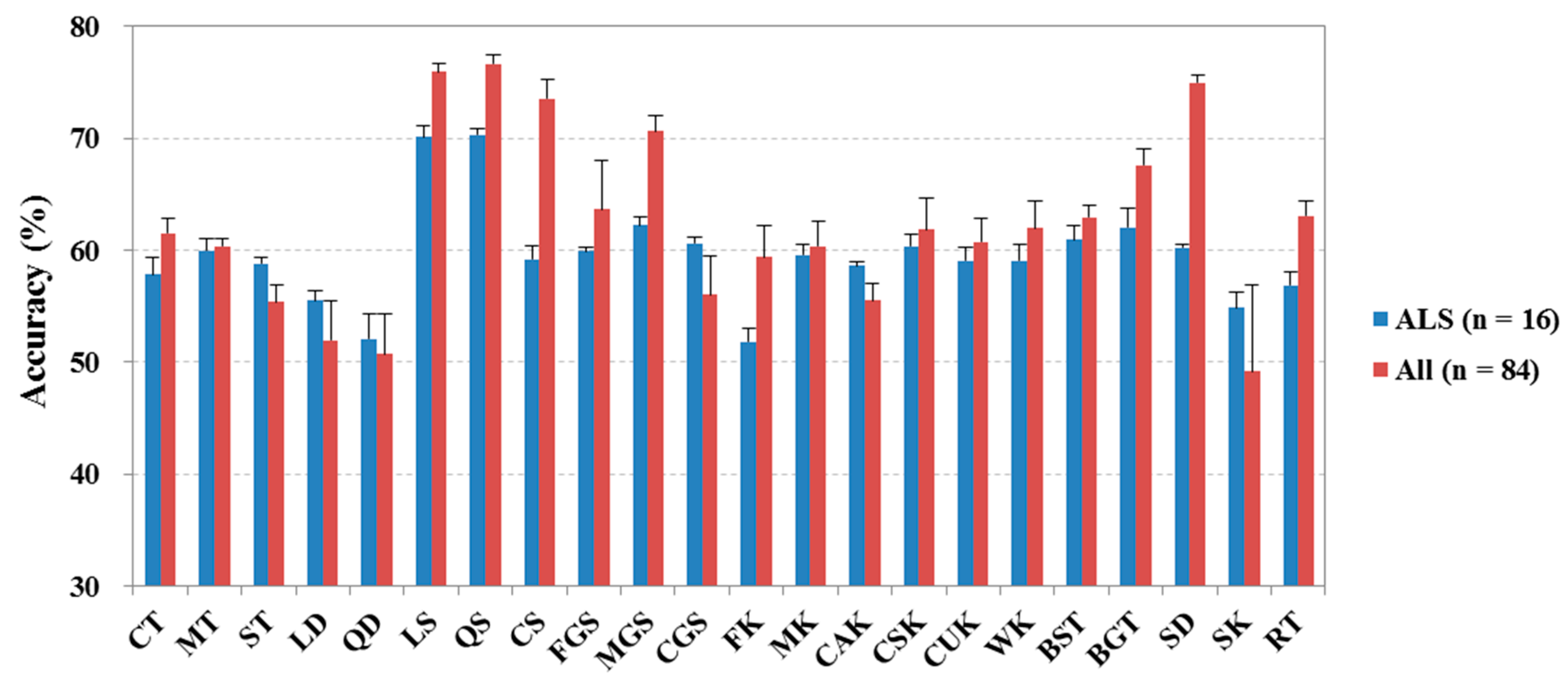
Table 4). CHA, CHPV and SI improved the overall accuracy by 5.5%, 1.4% and 0.4%, respectively. However, CA and CH only contributed 0.2% to the species classification. The best combination of features for species classification was determined using the QSVM approach, which indicates that there may be other best combinations for the NN and RF methods. In addition, the findings of this study did not support the recommendation that as many additional features as possible should be included in the tree species classification [44].
In this study, 22 algorithms were initially compared using 100 classifications, and the results indicated that the QSVM classifier had higher classification accuracies than the other classifiers. Then, the QSVM classifier was compared with the NN and RF approaches using eight combinations of different features. Previous studies obtained comparable results from the RF classifications [50,53,58,59], and some authors showed that RF produced higher classification accuracies than other classification techniques such as decision trees and bagging trees [61,
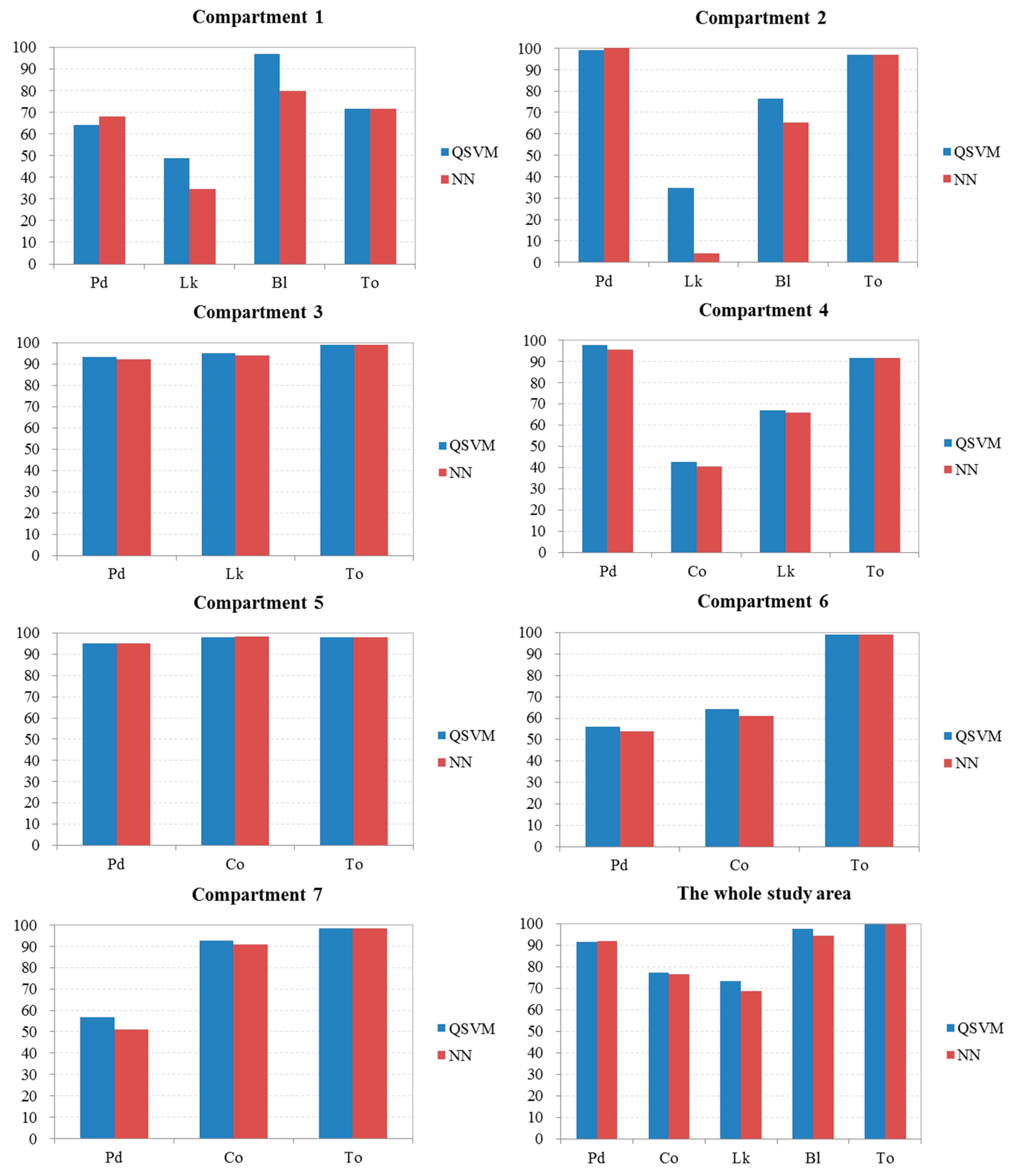
75]. In our study, however, we found that the QSVM and NN models were preferable to the RF models based on the classification accuracies. Although the overall accuracies of the classifications using NN were slightly higher than those using QSVM, it should be noted that several problems still remain with the NN method. For example, the NN model is more difficult to interpret than the QSVM model because it exhibits one or more hidden layer(s) and may therefore appear to be a “black box.” In terms of classification accuracies of different species, QSVM even obtained slightly better results than NN, especially for the broadleaved trees. Accordingly, we recommend the quadratic SVM approach rather than the neural network method to classify the tree crowns of forests in the study area. However, these classification approaches should be further compared in other forests using different data.
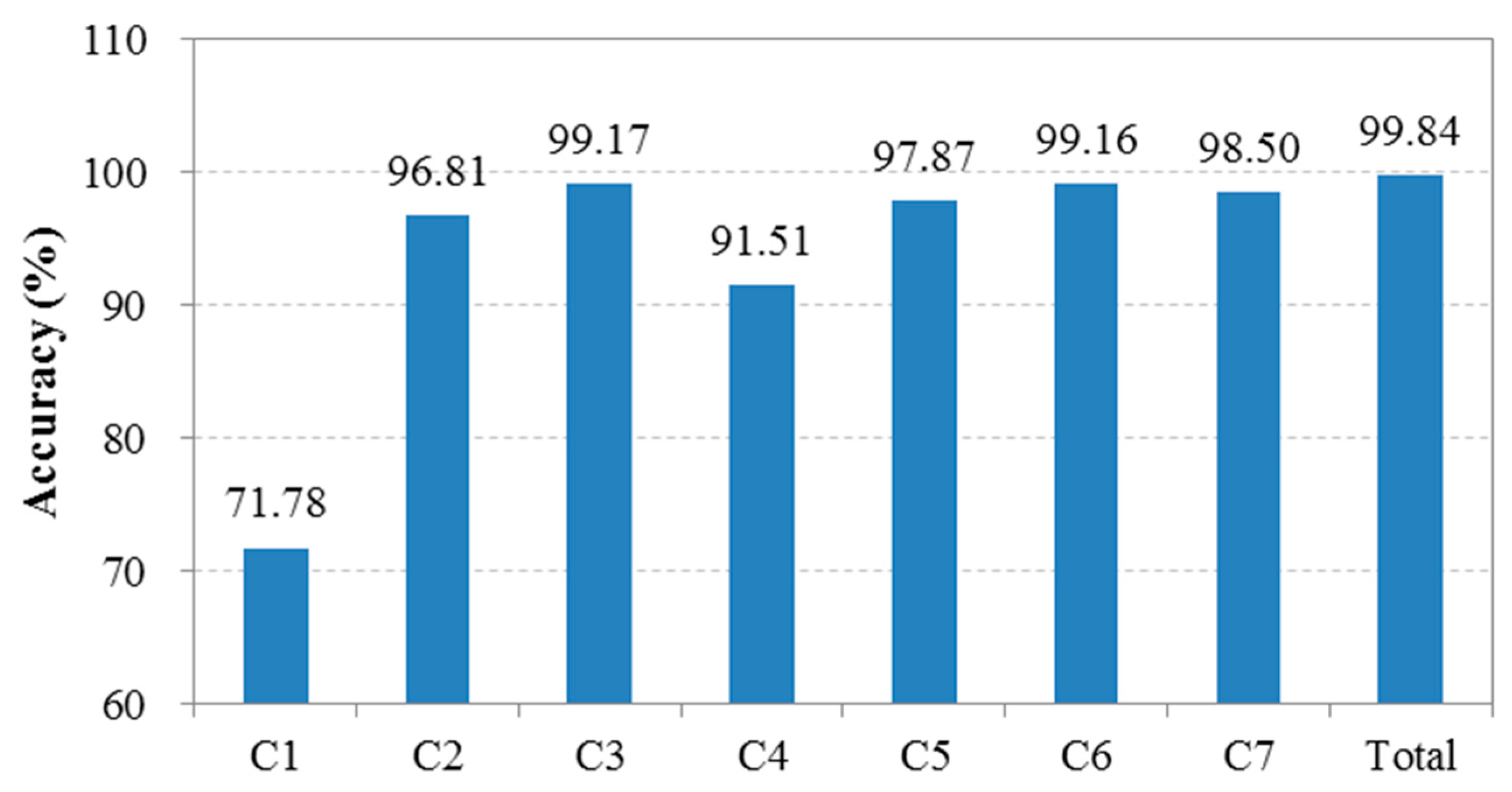
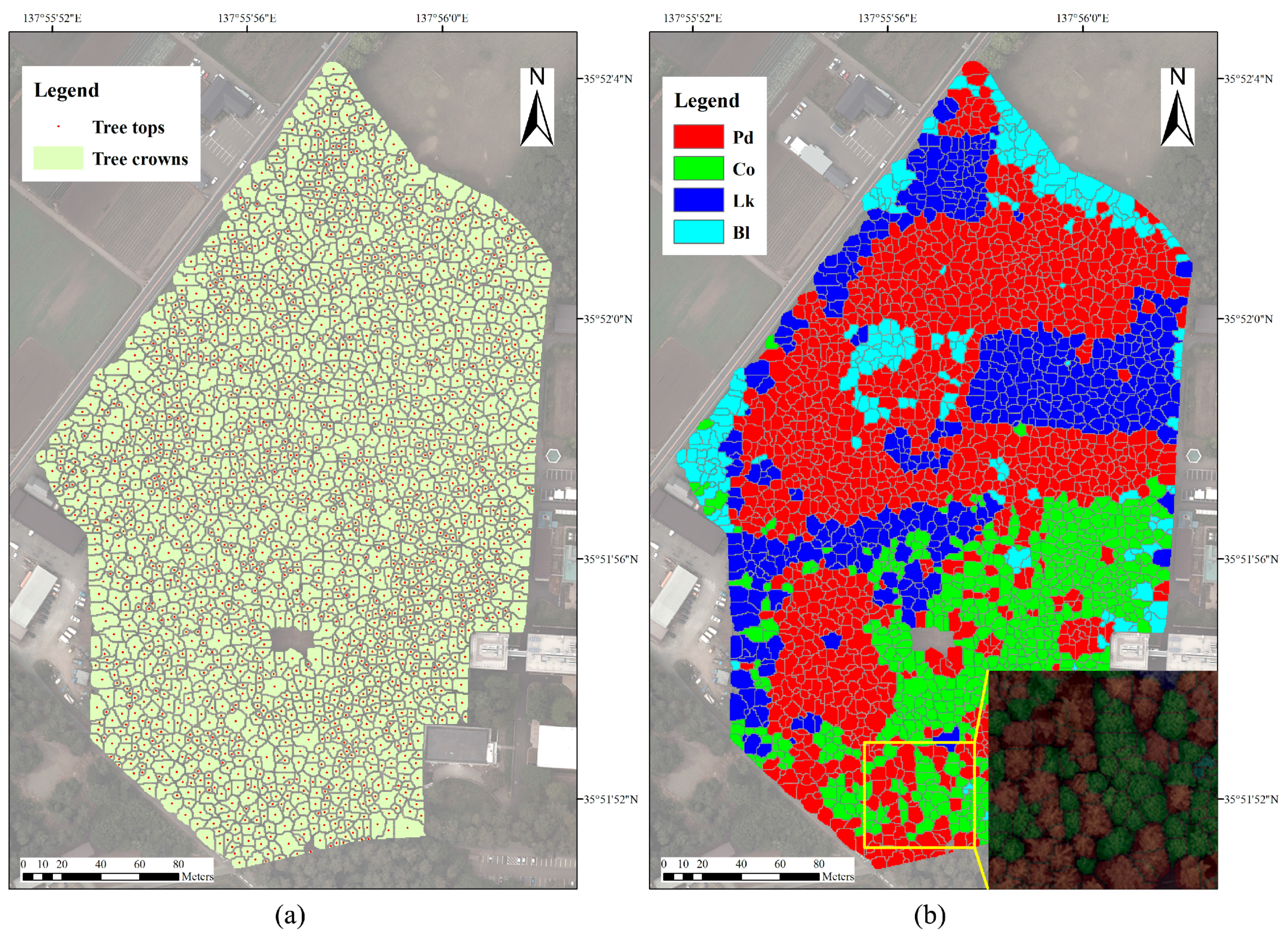
In theory, the success rate of individual tree detection to distinguish species depends on the accuracies of tree crown delineation and species classification in the study area. In this study, more than 90% of the trees in most compartments were delineated, and a classification accuracy of 90.8% was obtained by the QSVM approach when using the best combination of features. However, some dominant tree species were detected with a relatively low accuracy in some compartments. For example, Chamaecyparis obtusa was detected with an accuracy of less than 65% in compartments 4 and 6, and the Pinus densiflora trees were delineated at 57% in compartment 7. These results can be attributed to the high stem density and complex spatial structure of the forests in these areas, which increase the probability of overlap between tree crowns and were disadvantageous for species classification. Additionally, the DBH distribution also contributed to the detection accuracy. The compartments with a higher standard deviation for DBH classes had a lower accuracy. Another reason may be that the forest inventory data from 2005 to 2007 were used to examine the detection accuracy, whereas the airborne laser data were acquired in 2013. Although no management activities, such as thinning or timber harvest, were conducted since 2005, slightly better results were found in the accuracies calculated using the data surveyed in 2015 and 2016 for compartments 4 and 2 compared with those recorded in 2007. In addition, the trees with a DBH larger than 25 cm were considered to be the dominant canopy trees of the study area and were used to calculate the detection accuracy of the tree crowns to distinguish species. In fact, a notable difference in stand structure was found between some compartments. Consequently, a determination approach using the canopy trees in different forests should be further explored.
The synergy of laser scanning data with multi and/or hyperspectral images for individual tree detection to distinguish species has received more attentions in recent years [39,40,67]. However, although more than 50% of Japanese land has been covered by ALS data as of July 2013 [2], few airborne multispectral images with more than four bands are available in these areas. The successful launch of several commercial satellites such as GeoEye-1, WorldView-2 and WorldView-3 that can acquire images with a resolution less than 1 m provided a solution to this problem [4]. In addition, WorldView-4, which was just launched on 11 November 2016, can be expected to be an effective means for single tree crown identification because it has the capability to collect 30 cm resolution imagery with an accuracy of 3 m CE90 [76]. In fact, a combination of ALS data and WorldView-3 images has been successfully used for extracting the damaged trees caused by pine wood nematode in another study. Consequently, single tree delineation using the synergy of laser data and high resolution satellite imagery will be tested in our next study.

5. Conclusions

The best combination of features for species classification was identified using a forward iteration method. The findings of our study suggest that the combination of true-color (red-green-blue—RGB), laser intensity (LI), convex hull area (CHA), convex hull point volume (CHPV), shape index (SI), crown area (CA) and crown height (CH) yielded a higher classification accuracy than other combinations when using the quadratic support vector machines (QSVM) classifier. In addition, we found that for the same feature, there were different contribution degrees to species classification under different combinations. In terms of different classification algorithms, the findings from this study recommend the quadratic SVM approach rather than the neural network method to classify the tree crowns of forests in the study area. However, these classification approaches should be further compared in other forests using different data.

Acknowledgments

This study was supported by a Grant-in-Aid for Scientific Research from the Japan Society for the Promotion of Science (JSPS KAKENHI Grant Number JP16K18716). We gratefully acknowledge a number of students of Shinshu University for their support in the field and plot surveys. We would like to thank the members of the Forest Measurement and Planning Laboratory, Shinshu University, for their advice and assistance with this study. Moreover, we wish to express our heartfelt thanks to Jiaojun Zhu for his constructive suggestions for the manuscript. Finally, we wish to acknowledge the helpful comments from the anonymous reviewers and editors.

Author Contributions

Songqiu Deng and Xiaowei Yu conceived and designed the experiment; Masato Katoh and Juha Hyyppä coordinated the research projects and provided technical support and conceptual advice; Songqiu Deng and Masato Katoh performed the experiments and collected the data; Songqiu Deng, Xiaowei Yu and Tian Gao contributed the analysis tools; Songqiu Deng and Tian Gao analyzed the data. All of the authors helped in the preparation and revision of the manuscript.

Conflicts of Interest

The authors declare no conflict of interest.

References

  1. Learning Museum of the Forest and Forestry. Japanese Forests. Available online: http://www.shinrin-ringyou.com/forest_japan/kokuyu_minyu.php (accessed on 31 October 2016).
  2. Akiyama, T. Utility of LiDAR data. In Case Studies for Disaster’s Preventation Using Airborne Laser Data; Japan Association of Precise Survey and Applied Technology: Tokyo, Japan, 2013; p. 26. [Google Scholar]
  3. Kuplich, T.M. Classifying regenerating forest stages in Amazônia using remotely sensed images and a neural network. For. Ecol. Manag. 2006, 234, 1–9. [Google Scholar] [CrossRef]
  4. Deng, S.; Katoh, M.; Guan, Q.; Yin, N.; Li, M. Interpretation of forest resources at the individual tree level at Purple Mountain, Nanjing City, China, using WorldView-2 imagery by combining GPS, RS and GIS technologies. Remote Sens. 2014, 6, 87–110. [Google Scholar] [CrossRef]
  5. Gougeon, F.A.; Leckie, D.G. The individual tree crown approach applied to IKONOS images of a coniferous plantation area. Photogramm. Eng. Remote Sens. 2006, 72, 1287–1297. [Google Scholar] [CrossRef]
  6. Lefsky, M.A.; Cohen, W.B.; Acker, S.A.; Parker, G.G.; Spies, T.A.; Harding, D. LiDAR remote sensing of the canopy structure and biophysical properties of Douglas-fir western hemlock forests. Remote Sens. Environ. 1999, 70, 339–361. [Google Scholar] [CrossRef]
  7. Popescu, S.C.; Wynne, R.H.; Scrivani, J.A. Fusion of small-footprint LiDAR and multi-spectral data to estimate plot-level volume and biomass in deciduous and pine forests in Virginia, USA. For. Sci. 2004, 50, 551–565. [Google Scholar]
  8. Sun, G.; Ranson, K.J. Modeling LiDAR returns from forest canopies. IEEE Trans. Geosci. Remote Sens. 2000, 38, 2617–2626. [Google Scholar]
  9. Yu, X.; Hyyppä, J.; Holopainen, M.; Vastaranta, M.; Viitala, R. Predicting individual tree attributes from airborne laser point clouds based on random forest technique. ISPRS J. Photogramm. Remote Sens. 2011, 66, 28–37. [Google Scholar] [CrossRef]
  10. Hyyppä, J.; Kelle, O.; Lehikoinen, M.; Inkinen, M. A segmentation-based method to retrieve stem volume estimates from 3-D tree height models produced by laser scanners. IEEE Trans. Geosci. Remote Sens. 2001, 39, 969–975. [Google Scholar] [CrossRef]
  11. Næsset, E.; Gobakken, T. Estimation of above- and below-ground biomass across regions of the boreal forest zone using airborne laser. Remote Sens. Environ. 2008, 112, 3079–3090. [Google Scholar] [CrossRef]
  12. Shendryk, I.; Broich, M.; Tulbure, M.G.; Alexandrov, S.V. Bottom-up delineation of individual trees from full-waveform airborne laser scans in a structurally complex eucalypt forest. Remote Sens. Environ. 2016, 173, 69–83. [Google Scholar] [CrossRef]
  13. Zhao, K.G.; Popescu, S.; Nelson, R. LiDAR remote sensing of forest biomass: A scale in variant estimation approach using airborne lasers. Remote Sens. Environ. 2009, 113, 182–196. [Google Scholar] [CrossRef]
  14. Hayashi, M.; Yamagata, Y.; Borjigin, H.; Bagan, H.; Suzuki, R.; Saigusa, N. Forest biomass mapping with airborne LiDAR in Yokohama City. J. Jpn. Soc. Photogram. Remote Sens. 2013, 52, 306–315. [Google Scholar] [CrossRef]
  15. Kodani, E.; Awaya, Y. Estimating stand parameters in manmade coniferous forest stands using low-density LiDAR. J. Jpn. Soc. Photogram. Remote Sens. 2013, 52, 44–55. [Google Scholar] [CrossRef]
  16. Takejima, K. The development of stand volume estimation model using airborne LiDAR for Hinoki (Chamaecyparis obtusa) and Sugi (Cryptomeria japonica). J. Jpn. Soc. Photogram. Remote Sens. 2015, 54, 178–188. [Google Scholar] [CrossRef]
  17. Takahashi, T.; Yamamoto, K.; Senda, Y.; Tsuzuku, M. Predicting individual stem volumes of sugi (Cryptomeria japonica D. Don) plantations in mountainous areas using small-footprint airborne LiDAR. J. For. Res. 2005, 10, 305–312. [Google Scholar] [CrossRef]
  18. Holopainen, M.; Vastaranta, M.; Hyyppä, J. Outlook for the next generation’s precision forestry in Finland. Forests 2014, 5, 1682–1694. [Google Scholar] [CrossRef]
  19. Gougeon, F.A. A crown following approach to the automatic delineation of individual tree crowns in high spatial resolution aerial images. Can. J. Remote Sens. 1995, 21, 274–284. [Google Scholar] [CrossRef]
  20. Ke, Y.; Zhang, W.; Quackenbush, L.J. Active contour and hill climbing for tree crown detection and delineation. Photogramm. Eng. Remote Sens. 2010, 76, 1169–1181. [Google Scholar] [CrossRef]
  21. Erikson, M. Segmentation of individual tree crowns in color aerial photographs using region growing supported by fuzzy rules. Can. J. For. Res. 2003, 33, 1557–1563. [Google Scholar] [CrossRef]
  22. Leckie, D.G.; Gougeon, F.A.; Tinis, S.; Nelson, T.; Burnett, C.N.; Paradine, D. Automated tree recognition in old growth conifer stands with high resolution digital imagery. Remote Sens. Environ. 2005, 94, 311–326. [Google Scholar] [CrossRef]
  23. Wulder, M.; Niemann, K.O.; Goodenough, D.G. Local maximum filtering for the extraction of tree locations and basal area for high spatial resolution imagery. Remote Sens. Environ. 2000, 73, 103–114. [Google Scholar] [CrossRef]
  24. Chen, Q.; Baldocchi, D.; Gong, P.; Kelly, M. Isolating individual trees in a savanna woodland using small footprint LiDAR data. Photogramm. Eng. Remote Sens. 2006, 72, 923–932. [Google Scholar] [CrossRef]
  25. Kaartinen, H.; Hyyppä, J.; Yu, X.; Vastaranta, M.; Hyyppä, H.; Kukko, A.; Holopainen, M.; Heipke, C.; Hirschmugl, M.; Morsdorf, F.; et al. An international comparison of individual tree detection and extraction using airborne laser scanning. Remote Sens. 2012, 4, 950–974. [Google Scholar] [CrossRef] [Green Version]
  26. Dalponte, M.; Reyes, F.; Kandare, K.; Gianelle, D. Delineation of Individual Tree Crowns from ALS and Hyperspectral data: A comparison among four methods. Eur. J. Remote Sens. 2015, 48, 365–382. [Google Scholar] [CrossRef]
  27. Jakubowski, M.K.; Li, W.; Guo, Q.; Kelly, M. Delineating individual trees from LiDAR data: A comparison of vector- and raster-based segmentation approaches. Remote Sens. 2013, 5, 4163–4186. [Google Scholar] [CrossRef]
  28. Lu, X.; Guo, Q.; Li, W.; Flanagan, J. A bottom-up approach to segment individual deciduous trees using leaf-off LiDAR point cloud data. ISPRS J. Photogramm. Remote Sens. 2014, 94, 1–12. [Google Scholar] [CrossRef]
  29. Solberg, S.; Næsset, E.; Bollandsås, O.M. Single tree segmentation using airborne laser scanner data in a structurally heterogeneous spruce forest. Photogramm. Eng. Remote Sens. 2006, 72, 1369–1378. [Google Scholar] [CrossRef]
  30. Yu, X.; Litkey, P.; Hyyppä, J.; Holopainen, M.; Vastaranta, M. Assessment of low density full-waveform airborne laser scanning for individual tree detection and tree species classification. Forests 2014, 5, 1011–1031. [Google Scholar] [CrossRef]
  31. Li, W.; Guo, Q.; Jakubowski, M.K.; Kelly, M. A new method for segmenting individual trees from the LiDAR point cloud. Photogramm. Eng. Remote Sens. 2012, 78, 75–84. [Google Scholar] [CrossRef]
  32. Reitberger, J.; Schnörr, Cl.; Krzystek, P.; Stilla, U. 3D segmentation of single trees exploiting full waveform LiDAR data. ISPRS J. Photogramm. Remote Sens. 2009, 64, 561–574. [Google Scholar] [CrossRef]
  33. Eysn, L.; Hollaus, M.; Lindberg, E.; Berger, F.; Monnet, J.M.; Dalponte, M.; Kobal, M.; Pellegrini, M.; Lingua, E.; Mongus, D.; et al. A benchmark of LiDAR-based single tree detection methods using heterogeneous forest data from the Alpine Space. Forests 2015, 6, 1721–1747. [Google Scholar] [CrossRef] [Green Version]
  34. Larsen, M.; Eriksson, M.; Descombes, X.; Perrin, G.; Brandtberg, T.; Gougeon, F.A. Comparison of six individual tree crown detection algorithms evaluated under varying forest conditions. Int. J. Remote Sens. 2011, 32, 5827–5852. [Google Scholar] [CrossRef]
  35. Vauhkonen, J.; Ene, L.; Gupta, S.; Heinzel, J.; Holmgren, J.; Pitkänen, J.; Solberg, S.; Wang, Y.; Weinacker, H.; Hauglin, K.M.; et al. Comparative testing of single-tree detection algorithms under different types of forest. Forestry 2012, 85, 27–40. [Google Scholar] [CrossRef]
  36. Edson, C.; Wing, M.G. Airborne light Detection and Ranging (LiDAR) for individual tree stem location, height, and biomass measurements. Remote Sens. 2011, 3, 2494–2528. [Google Scholar] [CrossRef] [Green Version]
  37. Koch, B.; Heyder, U.; Weinacker, H. Detection of individual tree crowns in airborne LiDAR data. Photogramm. Eng. Remote Sens. 2006, 72, 357–363. [Google Scholar] [CrossRef]
  38. Yao, W.; Krzystek, P.; Heurich, M. Tree species classification and estimation of stem volume and DBH based on single tree extraction by exploiting airborne full-waveform LiDAR data. Remote Sens. Environ. 2012, 123, 368–380. [Google Scholar] [CrossRef]
  39. Dalponte, M.; Ørka, H.O.; Ene, L.T.; Gobakken, T.; Næsset, E. Tree crown delineation and tree species classification in boreal forests using hyperspectral and ALS data. Remote Sens. Environ. 2014, 140, 306–317. [Google Scholar] [CrossRef]
  40. Heinzel, J.; Koch, B. Investigating multiple data sources for tree species classification in temperate forest and use for single tree delineation. Int. J. Appl. Earth Obs. Geoinf. 2012, 18, 101–110. [Google Scholar] [CrossRef]
  41. Katoh, M.; Gougeon, F.A.; Leckie, D.G. Application of high-resolution airborne data using individual tree crown in Japanese conifer plantations. J. For. Res. 2009, 14, 10–19. [Google Scholar] [CrossRef]
  42. Coburn, C.A.; Roberts, A.C.B. A multiscale texture analysis procedure for improved forest stand classification. Int. J. Remote Sens. 2004, 25, 4287–4308. [Google Scholar] [CrossRef]
  43. Gao, T.; Zhu, J.; Zheng, X.; Shang, G.; Huang, L.; Wu, S. Mapping spatial distribution of larch plantations from multi-seasonal Landsat-8 OLI imagery and multi-scale textures using random forests. Remote Sens. 2015, 7, 1702–1720. [Google Scholar] [CrossRef]
  44. Li, J.; Hu, B.; Noland, T.L. Classification of tree species based on structural features derived from high density LiDAR data. Agric. For. Meteorol. 2013, 171–172, 104–114. [Google Scholar] [CrossRef]
  45. Holmgren, J.; Persson, Å. Identifying species of individual trees using airborne laser scanner. Remote Sens. Environ. 2004, 90, 415–423. [Google Scholar] [CrossRef]
  46. Ørka, H.O.; Næsset, E.; Bollandsås, O.M. Classifying species of individual trees by intensity and structure features derived from airborne laser scanner data. Remote Sens. Environ. 2009, 113, 1163–1174. [Google Scholar] [CrossRef]
  47. Vaughn, N.R.; Moskal, L.M.; Turnblom, E.C. Tree species detection accuracies using discrete point lidar and airborne waveform LiDAR. Remote Sens. 2012, 4, 377–403. [Google Scholar] [CrossRef]
  48. Lin, Y.; Hyyppä, J. A comprehensive but efficient framework of proposing and validating feature parameters from airborne LiDAR data for tree species classification. Int. J. Appl. Earth Obs. Geoinf. 2016, 46, 45–55. [Google Scholar] [CrossRef]
  49. Reitberger, J.; Krzystek, P.; Stilla, U. Analysis of full waveform LiDAR data for the classification of deciduous and coniferous trees. Int. J. Remote Sens. 2008, 29, 1407–1431. [Google Scholar] [CrossRef]
  50. Cao, L.; Coops, N.C.; Innes, J.L.; Dai, J.; Ruan, H.; She, G. Tree species classification in subtropical forests using small-footprint full-waveform LiDAR data. Int. J. Appl. Earth Obs. Geoinf. 2016, 49, 39–51. [Google Scholar] [CrossRef]
  51. Heinzel, J.; Koch, B. Exploring full-waveform LiDAR parameters for tree species classification. Int. J. Appl. Earth Obs. Geoinf. 2011, 13, 152–160. [Google Scholar] [CrossRef]
  52. Kankare, V.; Liang, X.; Vastaranta, M.; Yu, X.; Holopainen, M.; Hyyppä, J. Diameter distribution estimation with laser scanning based multisource single tree inventory. ISPRS J. Photogramm. Remote Sens. 2015, 108, 161–171. [Google Scholar] [CrossRef]
  53. Naidoo, L.; Cho, M.A.; Mathieu, R.; Asner, G. Classification of savanna tree species, in the Greater Kruger National Park region, by integrating hyperspectral and LiDAR data in a Random Forest data mining environment. ISPRS J. Photogramm. Remote Sens. 2012, 69, 167–179. [Google Scholar] [CrossRef]
  54. Li, J.; Hu, B. Exploring high-density airborne light detection and ranging data for classification of mature coniferous and deciduous trees in complex Canadian forests. J. Appl. Remote Sens. 2012, 6. [Google Scholar] [CrossRef]
  55. Colgan, M.S.; Baldeck, C.A.; Féret, J.-B.; Asner, G.P. Mapping savanna tree species at ecosystem scales using support vector machine classification and BRDF correction on airborne hyperspectral and LiDAR data. Remote Sens. 2012, 4, 3462–3480. [Google Scholar] [CrossRef]
  56. Yang, J.; Jones, T.; Caspersen, J.; He, Y. Object-based canopy gap segmentation and classification: Quantifying the pros and cons of integrating optical and LiDAR data. Remote Sens. 2015, 7, 15917–15932. [Google Scholar] [CrossRef]
  57. Breiman, L. Random Forests. Mach. Learn. 2001, 45, 5–32. [Google Scholar] [CrossRef]
  58. Lawrence, R.L.; Wood, S.D.; Sheley, R.L. Mapping invasive plants using hyperspectral imagery and Breiman Cutler classifications (randomForest). Remote Sens. Environ. 2006, 100, 356–362. [Google Scholar] [CrossRef]
  59. St-Onge, B.; Audet, F.-A.; Bégin, J. Characterizing the height structure and composition of a boreal forest using an individual tree crown approach applied to photogrammetric point clouds. Forests 2015, 6, 3899–3922. [Google Scholar] [CrossRef]
  60. Hovi, A.; Korhonena, L.; Vauhkonen, J.; Korpela, I. LiDAR waveform features for tree species classification and their sensitivity to tree- and acquisition related parameters. Remote Sens. Environ. 2016, 173, 224–237. [Google Scholar] [CrossRef]
  61. Li, M.; Im, J.; Beier, C. Machine learning approaches for forest classification and change analysis using multi-temporal Landsat TM images over Huntington Wildlife Forest. GISci. Remote Sens. 2013, 50, 361–384. [Google Scholar]
  62. Leckie, D.G.; Gougeon, F.A.; Hill, D.A.; Quinn, R.; Armstrong, L.; Shreenan, R. Combined high-density lidar and multispectral imagery for individual tree crown analysis. Can. J. Remote Sens. 2003, 29, 633–649. [Google Scholar] [CrossRef]
  63. Kankare, V.; Räty, M.; Yu, X.; Holopainen, M.; Vastaranta, M.; Kantola, T.; Hyyppä, J.; Hyyppä, H.; Alho, P.; Viitala, R. Single tree biomass modelling using airborne laser scanning. ISPRS J. Photogramm. Remote Sens. 2013, 85, 66–73. [Google Scholar] [CrossRef]
  64. Mathworks. Supervised Learning Workflow and Algorithms. Available online: http://jp.mathworks.com/help/stats/supervised-learning-machine-learning-workflow-and-algorithms.html?lang=en (accessed on 6 August 2016).
  65. Mathworks. Classify Patterns with a Neural Network. Available online: http://jp.mathworks.com/help/nnet/gs/classify-patterns-with-a-neural-network.html (accessed on 6 August 2016).
  66. Gao, T.; Zhu, J.; Deng, S.; Zheng, X.; Zhang, J.; Shang, G.; Huang, L. Timber production assessment of a plantation forest: An integrated framework with field-based inventory, multi-source remote sensing data and forest management history. Int. J. Appl. Earth Obs. Geoinf. 2016, 52, 155–165. [Google Scholar] [CrossRef]
  67. Matsuki, T.; Yokoya, N.; Iwasaki, A. Hyperspectral tree species classification of Japanese complex mixed forest with the aid of LiDAR data. IEEE J. Sel. Top. Appl. Earth Obs. Remote Sens. 2015, 8, 2177–2187. [Google Scholar] [CrossRef]
  68. Lee, J.; Cai, X.; Lellmann, J.; Dalponte, M.; Malhi, Y.; Butt, N.; Morecroft, M.; Schönlieb, C.B.; Coomes, D.A. Individual tree species classification from airborne multisensor imagery using robust PCA. IEEE J. Sel. Top. Appl. Earth Obs. Remote Sens. 2016, 9, 2554–2567. [Google Scholar] [CrossRef]
  69. Deng, S.; Katoh, M. Interpretation of forest resources at the individual tree level in Japanese conifer plantations using airborne LiDAR data. Remote Sens. 2016, 8. [Google Scholar] [CrossRef]
  70. Immitzer, M.; Atzberger, C.; Koukal, T. Tree species classification with random forest using very high spatial resolution 8-band WorldView-2 satellite data. Remote Sens. 2012, 4, 2661–2693. [Google Scholar] [CrossRef]
  71. Straub, C.; Weinacker, H.; Koch, B. A comparison of different methods for forest resource estimation using information from airborne laser scanning and CIR orthophotos. Eur. J. For. Res. 2010, 129, 1069–1080. [Google Scholar] [CrossRef]
  72. Mutanga, O.; Adma, E.; Cho, M.A. High density biomass estimation for wetland vegetation using WorldView-2 imagery and random forest regression algorithm. Int. J. Appl. Earth Obs. Geoinf. 2012, 18, 399–406. [Google Scholar] [CrossRef]
  73. Korpela, I.; Ørka, H.O.; Maltamo, M.; Tokola, T.; Hyyppä, J. Tree species classification using airborne LiDAR—Effects of stand and tree parameters, downsizing of training set, intensity normalization, and sensor type. Silva Fenn. 2010, 44, 319–339. [Google Scholar] [CrossRef]
  74. Kim, S.; McGaughey, R.J.; Andersen, H.E.; Schreuder, G. Tree species differentiation using intensity data derived from leaf-on and leaf-off airborne laser scanner data. Remote Sens. Environ. 2009, 113, 1575–1586. [Google Scholar] [CrossRef]
  75. Prasad, A.M.; Iverson, L.R.; Liaw, A. Newer classification and regression tree techniques: Bagging and random forests for ecological prediction. Ecosystems 2006, 9, 181–199. [Google Scholar] [CrossRef]
  76. DigitalGlobe. Meet WorldView-4. Available online: http://worldview4.digitalglobe.com/#/main (accessed on 10 December 2016).
Figure 1. A map of the study area showing field data collected from April 2005 to June 2007. DBH, diameter at breast height; Pd, Pinus densiflora; Co, Chamaecyparis obtusa; Lk, Larix kaempferi; Bl, broadleaved trees.
Remotesensing 08 01034 g001
Figure 2. Frequency distribution of all trees in the study area with a DBH larger than 5 cm. The x-axis shows the DBH class; for example, the “6” and “10” classes represent the trees with DBHs ranging from 5 to 7 cm and from 9 to 11 cm, respectively. The y-axis shows the number of trees included in each DBH class.
Remotesensing 08 01034 g002
Figure 3. Research flow chart. DEM, digital elevation model; DSM, digital surface model; CHM, canopy height model.
Remotesensing 08 01034 g003
Figure 4. A part of the CHM data before and after correction.
Remotesensing 08 01034 g004
Figure 5. Procedure used for individual tree detection and feature extraction. (a) Corrected CHM; (b) Gaussian-filtered image; (c) potential tree tops; (d) dilated tree tops; (e) watershed segmented tree crowns with tree tops; and (f) laser point clouds within an individual tree crown.
Remotesensing 08 01034 g005
Figure 6. Classification accuracy of the 22 algorithms using 16 and 84 sub-datasets randomly selected from the 17 ALS-derived data and all 23 features, respectively. CT, complex tree; MT, medium tree; ST, simple tree; LD, linear discriminant; QD, quadratic discriminant; LS, linear SVM; QS, quadratic SVM; CS, cubic SVM; FGS, fine Gaussian SVM; MGS, medium Gaussian SVM; CGS, coarse Gaussian SVM; FK, fine KNN; MK, medium KNN; CAK, coarse KNN; CSK, cosine KNN; CUK, cubic KNN; WK, weighted KNN; BST, boosted trees; BGT, bagged trees; SD, subspace discriminant; SK, subspace KNN; RT, RUSBoosted trees.
Remotesensing 08 01034 g006
Figure 7. The detected accuracy of the tree crowns in different compartments and in the whole study area.
Remotesensing 08 01034 g007
Figure 8. Delineated tree crowns and tree tops using the CHM data (a); and manually identified tree species (b). Pd, Pinus densiflora; Co, Chamaecyparis obtusa; Lk, Larix kaempferi; Bl, broadleaved trees.
Remotesensing 08 01034 g008
Figure 9. A bar chart representing the producer and user accuracies for the three classifications of tree crowns classified using the quadratic SVM (QSVM), neural network (NN), and random forest (RF) approaches with the highest overall accuracy. Pd, Pinus densiflora; Co, Chamaecyparis obtusa; Lk, Larix kaempferi; Bl, broadleaved trees; PA, producer accuracy; UA, user accuracy.
Remotesensing 08 01034 g009
Figure 10. Tree crown classification based on the quadratic SVM (a) and neural network (b) models. Pd, Pinus densiflora; Co, Chamaecyparis obtusa; Lk, Larix kaempferi; Bl, broadleaved trees.
Remotesensing 08 01034 g010
Figure 11. A comparison of the accuracies of the dominant tree species in each compartment and the entire study area interpreted using the quadratic SVM (QSVM) and neural network (NN) approaches. Pd, Pinus densiflora; Co, Chamaecyparis obtusa; Lk, Larix kaempferi; Bl, broadleaved trees; To, total accuracy of the detected tree crowns versus the surveyed trees.
Remotesensing 08 01034 g011
Table 1. Characteristics of the forests at the study site surveyed from April 2005 to June 2007. DBH, diameter at breast height. Pd, Pinus densiflora; Co, Chamaecyparis obtusa; Lk, Larix kaempferi; Bl, broadleaved trees. a stem density of the trees with a DBH larger than 5 cm; b stem density of the trees with a DBH larger than 25 cm (the upper trees).
Compartment (Area, ha)Dominant SpeciesMin DBH (cm)Max DBH (cm)Average DBH (cm)Average Height (m)Density a (Stem/ha)Density b (Stem/ha)Basal Area (m2/ha)
1 (0.67)Pd, Lk, Bl5.459.022.815.258324531.0
2 (1.06)Pd, Lk, Bl7.456.921.815.982229939.1
3 (1.10)Pd, Lk5.058.722.316.774432837.4
4 (1.39)Pd, Co, Lk5.077.122.216.295440549.6
5 (1.10)Pd, Co5.081.624.316.577538546.8
6 (1.22)Pd, Co6.863.623.615.971029442.6
7 (0.73)Pd, Co7.765.326.317.463236241.8
Table 2. Features and variables extracted from the airborne laser (ALS) data and orthoimages for all trees.
RS SourcesFeaturesDescription
True-color (RGB) orthoimagesRavgThe average value of the red band within each segment
RsdThe standard deviation of the red band within each segment
GavgThe average value of the green band within each segment
GsdThe standard deviation of the green band within each segment
BavgThe average value of the blue band within each segment
BsdThe standard deviation of the blue band within each segment
Airborne laser data (ALS)Laser intensity (LI)The average laser intensity within each segment
Convex hull area (CHA)The area of the convex hull of each segment
Convex hull point volume (CHPV)The volume of the crown points within the convex hull of each segment
Shape index (SI)The ratio of the area to the perimeter of each segment
Crown area (CA)The area of each segment
Crown height (CH)The difference between the highest and lowest pixels of the CHM within each segment
Crown slope (CS)The average slope value of the CHM within each segment
Convex hull point density (CHPD)The point density of the crown points within the convex hull of each segment
Crown point density (CPD)The point density of the crown points within each segment
Crown point volume (CPV)The volume of the crown point clouds within each segment
Convex hull volume (CHV)The volume of the convex hull of each segment derived from the CHM
Convex hull surface area (CHSA)The surface area of the convex hull of each segment derived from the CHM
Convex hull diameter (CHD)The diameter of a circle with an area equal to the convex hull of each segment
Crown volume (CV)The crown volume of each segment derived from the CHM
Crown surface area (CSA)The surface area of each segment derived from the CHM
Crown diameter (CD)The diameter of a circle with an area equal to each segment
Tree height (TH)Estimated using the highest laser point within each segment
Table 3. Classification methods with different algorithms used in this study.
MethodAlgorithm
Decision trees (DT) aComplex tree
Medium tree
Simple tree
Discriminant analyses (DA) aLinear discriminant
Quadratic discriminant
Support vector machines (SVM) aLinear SVM
Quadratic SVM
Cubic SVM
Fine Gaussian SVM
Medium Gaussian SVM
Coarse Gaussian SVM
K-nearest neighbors classifiers (KNN) aFine KNN
Medium KNN
Coarse KNN
Cosine KNN
Cubic KNN
Weighted KNN
Ensemble classifiers (EC) aBoosted trees
Bagged trees
Subspace discriminant
Subspace KNN
RUSBoosted trees
Neural network (NN) bTwo-layer feed-forward network
Random forest (RF) cRegression tree
Notes: a for detailed information refer to [64]; b for detailed information refer to [65]; c for detailed information refer to [57].
Table 4. Overall accuracy (%) of the quadratic SVM classifications using different features and increments compared to the highest accuracy in each previous loop. ACC, accuracy; INC, increment. The feature abbreviations are the same as in Table 2.
FeatureACCINCACCINCACCINCACCINCACCINCACCINCACCINC
RGB76.7-------------
LI83.36.6------------
CHA81.75.088.85.5----------
CHPV82.05.387.54.290.21.4--------
SI81.95.287.34.090.01.290.60.4------
CA81.54.886.73.489.91.190.40.290.70.1----
CH80.13.485.82.589.10.389.7−0.590.4−0.290.80.1--
CS80.33.684.81.589.50.789.3−0.989.2−1.489.2−1.589.5−1.3
CHPD77.81.183.90.689.10.388.6−1.689.7−0.989.3−1.489.2−1.6
CPD77.00.383.80.588.4−0.488.8−1.489.1−1.589.5−1.288.6−2.2
CPV80.74.084.51.289.70.990.20.090.3−0.390.2−0.589.6−1.2
CHV79.93.285.11.889.30.589.2−1.089.5−1.190.0−0.789.5−1.3
CHSA80.33.685.32.088.90.188.9−1.389.2−1.489.1−1.689.7−1.1
CHD79.73.084.41.189.30.589.6−0.690.3−0.390.2−0.590.3−0.5
CV80.74.085.42.189.20.490.0−0.289.5−1.190.0−0.789.7−1.1
CSA78.21.584.91.689.50.788.8−1.489.2−1.489.3−1.489.6−1.2
CD79.22.586.02.789.60.889.5−0.789.6−1.090.0−0.790.3−0.5
TH76.90.283.30.088.80.088.6−1.688.9−1.788.8−1.989.5−1.3
Table 5. Overall accuracy (%) and kappa coefficient of the QSVM, NN and RF classifications obtained using different tree features. OA, overall accuracy; KC, kappa coefficient. Other abbreviations are the same as in Table 2 and Table 3.
DatasetQSVMNNRF
OAKCOAKCOAKC
RGB76.70.6381.60.7275.90.62
RGB + LI83.30.7486.70.8083.90.74
RGB + LI + CHA88.80.8389.50.8484.40.75
RGB + LI + CHA + CHPV90.20.8590.60.8684.30.75
RGB + LI + CHA + CHPV + SI90.60.8691.00.8684.50.75
RGB + LI + CHA + CHPV + SI + CA90.70.8689.80.8484.70.76
RGB + LI + CHA + CHPV + SI + CA + CH90.80.8689.30.8384.30.75
All features87.60.8190.20.8583.20.73
Table 6. Count of the upper trees surveyed in the field data and classified using different approaches based on distinguishing species. QSVM, quadratic SVM classifier; NN, neural network; Pd, Pinus densiflora; Co, Chamaecyparis obtusa; Lk, Larix kaempferi; Bl, broadleaved trees.
CompartmentSpeciesField DataQSVMNNCompartmentSpeciesField DataQSVMNN
1Pd5068665Pd167175175
Co-511Co235230231
Lk497481Lk376
Bl646251Bl182020
Total163209209Total423432432
2Pd2512532516Pd143206209
Co1612Co190122116
Lk233845Lk183130
Bl554236Bl837
Total345334334Total359362362
3Pd1821701687Pd517376
Co434Co207192188
Lk169177179Lk112
Bl576Bl744
Total360357357Total266270270
4Pd263257251AllPd110712021196
Co1436158Co795614610
Lk88117118Lk351445461
Bl243947Bl181177171
Total518474474Total243424382438
Table 7. Error matrices for the matching tests between detected and surveyed trees. Pd, Pinus densiflora; Co, Chamaecyparis obtusa; Lk, Larix kaempferi; Bl, broadleaved trees.
MethodClass NameField DataTotalCommission Accuracy (%)Overall Accuracy (%)
PdCoLkBl
QSVMPd1214391517128594.589.4
Co48545233264884.1
Lk16115202757490.6
Bl12343230738579.7
Total12906295903832892
Omission Accuracy (%)94.186.688.180.2
NNPd1191423734130491.387.6
Co35540312463085.7
Lk25184972056088.8
Bl39292530539876.6
Total12906295903832892
Omission Accuracy (%)92.385.984.279.6

