A New Operational Snow Retrieval Algorithm Applied to Historical AMSR-E Brightness Temperatures

Abstract

Snow is a key element of the water and energy cycles and the knowledge of spatio-temporal distribution of snow depth and snow water equivalent (SWE) is fundamental for hydrological and climatological applications. SWE and snow depth estimates can be obtained from spaceborne microwave brightness temperatures at global scale and high temporal resolution (daily). In this regard, the data recorded by the Advanced Microwave Scanning Radiometer—Earth Orbiting System (EOS) (AMSR-E) onboard the National Aeronautics and Space Administration’s (NASA) AQUA spacecraft have been used to generate operational estimates of SWE and snow depth, complementing estimates generated with other microwave sensors flying on other platforms. In this study, we report the results concerning the development and assessment of a new operational algorithm applied to historical AMSR-E data. The new algorithm here proposed makes use of climatological data, electromagnetic modeling and artificial neural networks for estimating snow depth as well as a spatio-temporal dynamic density scheme to convert snow depth to SWE. The outputs of the new algorithm are compared with those of the current AMSR-E operational algorithm as well as in-situ measurements and other operational snow products, specifically the Canadian Meteorological Center (CMC) and GlobSnow datasets. Our results show that the AMSR-E algorithm here proposed generally performs better than the operational one and addresses some major issues identified in the spatial distribution of snow depth fields associated with the evolution of effective grain size.

1. Introduction

Snow is a key element of the water and energy cycles and the knowledge of bulk snow properties at both local and global scales is crucial for hydrological and climatological applications. Because its radiative and thermal properties modulate transfers of energy and mass at the surface–atmosphere interface [1], snow affects the overlying atmosphere [2,3] and thereby plays an important role in the complex web of feedbacks that control local to global climate. Snow also modulates the hydrologic cycle [4,5], influences ecosystem functioning [6] and is a significant resource for many mid latitude populations and for populations whose water is derived from mountainous and northerly cold regions [7,8]. Moreover, knowledge of snow depth or snow water equivalent (SWE) is fundamental for water resources management, weather forecast and flashflood predictions. Further, snow strongly influences the global energy balance because of its high reflectivity, insulation properties, and the large amount of latent heat consumed during melting.

Snow depth is routinely measured by automatic weather stations (AWS) or by other in-situ sensors (such as snow pillows). Although extremely valuable and precious for regional and local scale applications, in-situ point-scale measurements are limited by their spatial coverage, with often only snow depth, and not SWE, being recorded at many locations. Remote sensing offers the unique opportunity to overcome the abovementioned spatial coverage limitations. In particular, spaceborne passive microwave data can be used to estimate snow depth and SWE at large spatial scales and high-temporal resolution, having been measuring the natural upwelling microwave radiation from the Earth for more than 35 years [9,10]. For snow covered terrains, the radiation emitted from a snowpack in the microwave region depends on the kinetic temperature of the snow, snow grain size, the number of grains in the path of the emitted radiation and their volume to air fraction, the underlying surface conditions and in-situ vegetation characteristics [11]. Several algorithms for the retrieval of SWE or snow depth have been proposed in the literature [12,13], reviewed and updated for forested areas [14,15,16,17,18,19]. Studies have also been conducted for improving the estimation of SWE at regional scale and through the use of numerical techniques for the inversion of semi-empirical relationships [20,21,22,23]. Grippa et al. [24], for example, used a dynamic algorithm to estimate seasonal SWE in Siberia and several dynamic algorithms have been proposed [25,26]. More recent algorithms rely on electromagnetic modeling [27,28] and assimilation approaches [29,30]. It has been demonstrated that the combination of space-borne passive microwave data with in-situ observations in an assimilation scheme improves the snow depth and SWE retrieval accuracy with respect to the case when only interpolation of synoptic surface observations is used [22]. The retrieval of snow depth from passive microwave brightness temperatures can be improved by using retrieval approaches that dynamically combine ancillary snow depth information (e.g., from snow physical models driven with surface meteorological data) when compared to established algorithms based solely on regression or electromagnetic modeling without ancillary inputs [26].

Until its failure on 4 October 2011 estimates of daily, pentad and monthly SWE and snow covered area (SCA) at global scale were produced operationally by NASA from the brightness temperatures measured by the Advanced Microwave Scanning Radiometer for EOS (AMSR-E) on the NASA’s AQUA spacecraft [31]. The AMSR-E was successfully launched on 4 May 2002, providing more than ten years of data that complement those acquired by other space-borne microwave sensors such as the Special Sensor Microwave Imager (SSM/I, [9]). The AMSR-E sensor is a twelve-channel, six-frequency total power passive microwave radiometer system, acquiring brightness temperatures at horizontal and vertical polarization at 6.9 GHz, 10.7 GHz, 18.7 GHz, 23.8 GHz, 36.5 GHz and 89.0 GHz [32]. At a nominal altitude of 705 km, the sensor measured the upwelling brightness temperatures over an angular sector of ±61° about the sub-satellite track, resulting in a swath width of ~1500 km. A summary of the performance characteristics of the AMSR-E is reported (

Table 1. Advanced Microwave Scanning Radiometer–Earth Orbiting System (AMSR-E) performance characteristics.

Center Freq (GHz)	6.9	10.7	18.7	23.8	36.5	89.0
Band Width (MHz)	350	100	200	400	1000	3000
Sensitivity (K)	0.3	0.6	0.6	0.6	0.6	1.1
IFOV (km × km)	76 × 44	49 × 28	28 × 16	31 × 18	14 × 8	6 × 4
Sampling Rate (km × km)	10 × 10	10 × 10	10 × 10	10 × 10	10 × 10	5 × 5
Integration Time (ms)	2.6	2.6	2.6	2.6	2.6	1.3
Main Beam Efficiency (%)	95.3	95.0	96.4	96.4	95.3	96.0
Beam Width (deg)	2.2	1.4	0.8	0.9	0.4	0.18

) [32]. The brightness temperature fields used in this study are provided by National Snow and Ice Data Center (NSIDC) in EASE-Grid projection [33].

During and after the AMSR-E lifetime, NASA supported the development, refinement and implementation of the NASA operational AMSR-E SWE product [31], the only NASA satellite-based SWE product available to the scientific community. The effort continues with the launch of the Advanced Microwave Scanning Radiometer 2 (AMSR2, [34]) onboard the GCOM-W1 satellite of the Japanese Aerospace Exploration Agency (JAXA) in 2012, collecting data at the same frequencies of AMSR-E, thus making possible the production of a long-term SWE product estimated from passive microwave datasets. Because of this, and to provide improved estimates of SWE at global scale, historical AMSR-E data can be re-processed using refined algorithms that can ultimately replace or complement the operational one used to produce the data currently distributed by NSIDC. Focusing on improving the ASMR-E SWE estimates will benefit also the retrieval of the same parameters using data collected either from SSM/I or from the Scanning Multi-channel Microwave Radiometer (SMMR), hence offering the possibility of improved estimates of SWE for more than three decades.

Here, we report the analysis of the performance of a new operational algorithm for re-processing NASA AMSR-E brightness temperatures and for estimating SWE at global scale. The new algorithm aims at addressing several issues identified through the analysis of the outputs of the current operational AMSR-E SWE product. Specifically, the new algorithm here proposed addresses, among other things, the overestimation of snow depth and SWE over Siberia, where large snow grains occurring throughout the season are not accounted for by the current operational algorithm. The new algorithm builds on the previous operational algorithm but combines the outputs of an electromagnetic modeling with artificial neural networks for estimating snow depth, snow surface temperature and the so-called effective snow grains (e.g., the size of the scatterers in the microwave region integrated along the penetration depth). Moreover, differently from the original operational algorithm, in the new algorithm snow density is not static, but it is dynamically computed (spatially and temporally), building on Sturm et al. [17].

2. Considerations on the Retrieval of SWE from Microwave Brightness Temperatures and Physical Basis

Under an electromagnetic point of view, dry snow can be approximated as a mixture of ice and air, with its permittivity depending on the permittivity of the single constituent materials and on their fractional volume. The real part of dry snow permittivity can be assumed to be constant with frequency and temperature and mainly depending on the snow fractional volume [11]. Dry or frozen ground are good emitters and the microwave signal recorded by passive microwave sensors over a snow covered terrain can be seen, in simple terms, as the signal naturally emitted by the underlying soil attenuated by the snow layer. The contribution from the dry snow layer itself is negligible because of the low emissivity of dry snow. The attenuation of the microwave signal for dry snow covered terrain is due to the multiple scattering occurring in the snowpack [11,35]. This is caused by dielectric discontinuities between snow grains and air [36] because the wavelengths in the microwave regions of interest (e.g., Ka and K bands) are comparable to the snow grain size. As a consequence of the low absorption in the case of dry snow, microwaves will penetrate and scatter over distances within the snowpack that are greater than the wavelength, hence resulting in volume scattering. Internal layers along the snowpack are also responsible for attenuation and scattering. Scattering increases with grain size and frequency [37], with multiple scattering further increasing the attenuation of the radiation emitted by the soil in the snow pack. Because the attenuation is related to the scatterers (e.g., snow grains) and this can be associated, in first approximation, to snow depth (e.g., the deeper the snow the more the scatterers, assuming a uniform distribution of snow grains with a given size [38,39]), an inverse relationship between snow depth and brightness temperature has been hypothesized for retrieval purposes. Because of the dense packing of the ice particles (with respect to the wavelength), the independent scattering assumption cannot be used and several theoretical models have been proposed in the literature to account for this [38,39,40]. Moreover, snow crystals tend to cluster in a snowpack after extended metamorphosis. By applying a “stickiness” parameter [41], it is possible to account for the clustering of non-spherical snow grains in the snowpack. However, the absence of measurements for such parameter and the difficulty in measuring it in the field makes it problematic to use it for operational purposes.

The microwave bands available on spaceborne sensors that are used for the retrieval are, generally, near K- (~19 GHz) and Ka-band (~37 GHz). Other sensors also collect data at C-band (~6 GHz) and X-band (~10 GHz), as in the case of the AMSR-E and SMMR, which can be used to address issues related to deep snow, as it will be discussed in the following. Early studies indicate that when snow depth exceeds 5 cm (or SWE exceeds 10 mm), scattering of naturally emitted microwave radiation can be detected at frequencies greater than 25 GHz [13]. Many of the retrieval algorithms used to estimate SWE from spaceborne passive microwave data have relied on the assumption that brightness temperature at K-band (~19 GHz) is weakly affected by the presence of the snowpack on ground but the Ka-band (~37 GHz) is more sensitive to the snow presence. Hence, snow depth and SWE estimates have been historically performed using the difference of the brightness temperature at the two frequencies [13,14]. However, for relatively deep snow and/or snow with relatively large grains (e.g., hoar) this assumption does not hold any longer, with the brightness temperature values at K-band also becoming affected by the presence of the snowpack [42]. Another limiting factor in estimating snow depth and SWE from passive microwave data is the presence of liquid water [43]. This increases absorption, with the consequence of reducing the penetration depth. As a consequence, the signal from the underlying soil does not reach the sensor and the measured brightness temperature is mainly associated with the emission from the wet surface of the snowpack. In wet snow conditions, therefore, the retrieval of snow depth, and consequently SWE, is not possible [13,14,15,16,17,18,19].

A crucial aspect of the retrieval of snow depth and SWE from spaceborne passive microwave data concerns the sensitivity of the data to grain size and snow density, being higher than that to snow depth. This makes the practical task of snow depth and SWE retrieval more challenging and ill-posed in its nature. An ill-posed problem is characterized by the conditions that it is not possible to affirm that the solution always exists; that if the solution exists then it is not unique; and that different sets of snow parameters may correspond to the same set of brightness temperatures and a small change in the problem may lead to a big change in the solution. The ill-posed nature of the problem in the case of snow depth/SWE retrieval from microwave data is reflected in the fact that there are several combinations of snow parameters that can correspond to a given set of measured brightness temperatures, given the errors associated with measurements and retrieval. For example, a relatively shallow snowpack with large grains can have brightness temperatures similar to the ones of a thicker snowpack, but with relatively smaller grains. Though the brightness temperatures in the two examples can be different from a theoretical point of view (when considering decimal places, for example), such difference is small when compared to the magnitude of the error associated to the data and to the convergence criteria associated to the minimization techniques (which can be of the order of Kelvins, depending on atmospheric conditions, snow properties and retrieval scheme). Without a-priori knowledge of the snowpack conditions (e.g., shallow with large grains vs. deep with small grains) the solution computed, for example, from the minimization of the difference between measured and modeled brightness temperatures might not be stable around a minimum and small perturbations in the input (e.g., the measured minus modeled brightness temperature) could reflect into large changes in the output (e.g., estimated snow parameters). The current operational algorithm, as we will see, does not account for this aspect and this represents a large source of error. Several approaches have been addressing this aspect, with studies assimilating ancillary information into remote sensing retrieval schemes. For example, Takala et al. [23] proposed an algorithm assimilating synoptic weather station data on snow depth with satellite passive microwave data to produce a 30-year-long time-series of seasonal SWE for the northern hemisphere, pointing out to the benefits of the developed assimilation approach with respect to a stand-alone passive microwave data algorithm.

Beside the abovementioned issues, there are other aspects that can impact the retrieval of SWE from spaceborne passive microwave data. Snow depth cannot be retrieved if it exceeds the penetration depth of the electromagnetic radiation. This is, in turn, a function of several factors and can range considerably depending on snow parameters, such as grain size and density and their vertical distribution. We refer to this as the saturation effect and it is responsible for an underestimation of snow depth (and SWE consequently) from the passive microwave data. Another limiting factor is related to the presence of forest within the area under observation. Forests, indeed, attenuate the radiation emitted by the underlying snowpack and, consequently, increase uncertainty on the SWE retrieval [14,20]. SWE retrieval is also affected by strong temperature gradient between liquid and frozen water in the presence of water bodies within a pixel [44] and by atmospheric components such as oxygen and cloud liquid water content [45]. Lastly, another important feature that affects the microwave response from snow is layering. Current retrieval algorithms generally consider the snowpack as a single layer of scatterers, whereas in reality, the presence of layers, ice lenses and the vertical distribution of snow properties can considerably affect not only the absolute brightness temperature values but also their polarization difference [46]. However, the inclusion of multiple layers in a retrieval scheme purely based on measured brightness temperature values is computationally consuming and requires the knowledge of the vertical distribution of snow properties.

3. Materials and Methods

3.1. Description of the Current Operational Retrieval Algorithm

The first SWE retrieval algorithms developed for spaceborne passive microwave data [13,14,47] were based on a linear regression between snow depth and the difference between brightness temperatures at ~19 (Tb19) and ~37 GHz (Tb37) (or similar frequencies, Equation (1)), with Tb19 and Tb37 expressed in Kelvin [K]. The regression coefficient (denoted as Rc) was static both in space and time and set to 1.6 cm/K for snow depth (SD) (assuming fixed value of mean grain radius of 0.3 mm). SWE was then derived assuming a fixed snow density of 0.3 g/cm³.

$$SD=Rc \times \left(Tb19-Tb37\right)$$

(1)

The algorithm was later modified to account for the attenuation introduced by forest cover (Equation (2)), [14] by dividing Rc by (1 − ff), where ff represents the forest cover fraction (ranging between 0 and 1).

$$SD=Rc \times \frac{1}{1-ff} \times \left(Tb19-Tb37\right)$$

(2)

The current AMSR-E SWE operational algorithm was built on this original effort and was developed at the NASA Goddard Space Flight Center [48]. Static ancillary datasets were introduced and consisted of global forest fraction Boston University IGBP data (MOD12Q11IGBP) [49], global forest density (University of Maryland’s (UMD) Vegetation Continuous Fields (VCF) based on MOD09A1), Land, Ocean Coasts & Ice Mask (derived from Moderate Resolution Imaging Spectroradiometer (MODIS) MOD12Q1 IGBP land cover data). A snow possible/not possible mask based on snow climatology data [50] was also introduced to account for the presence/absence of snow. For reader’s convenience, the sources of ancillary data are provided in

Table 2. Ancillary datasets required by AMSR-E SWE operational algorithm.

Data Set	Source
Global Forest Fraction	Boston University IGBP data (MOD12Q11GBP) (Hansen et al., 2003)
Global Forest Density	UMD/VCF (based on MOD09A1)
Land, Ocean Coasts & Ice Mask	Derived from MODIS MOD12Q1 IGBP land cover data (collection V004)
Snow possibility/impossibility	Snow climatology data set (Dewey and Heim, 1984)
Snow density	Seasonal snow classification map (Liston and Sturm, 1998)

. The flowchart diagram of the AMSR-E SWE operational algorithm is reported in Figure 1.

In order to separate dry from wet snow conditions, an absolute brightness temperature threshold method is applied. In the following, we will denote the brightness temperature values at different frequencies and polarizations as TbFreqPol (e.g., Tb36 H denotes the brightness temperature measured at 36.5 GHz, horizontal polarization). In the AMSR-E operational algorithm, dry snow is assumed to be present if both conditions of Tb36 H < 245 K and Tb36 V < 255 K are satisfied [48]. If dry snow is present and if Tb10 V − Tb36 V > 0 K or Tb10 H − Tb36 H > 0 K, then medium to deep snow is assumed to be present. However, if Tb10 V − Tb36 V ≤ 0 K and Tb10 H − Tb36 H ≤ 0 K snow is still possible but it is assumed to be shallow if Tb89 V ≤ 255 K, Tb89 H ≤ 265 K, Tb23 V − Tb89 V > 0 K, Tb23 H − Tb89 V > 0 K and Tsnow < 267 K. Here Tsnow is the snowpack surface temperature obtained using a combination of brightness temperatures [25]. In case shallow snow is detected, snow depth is set to 5 cm [48]. If medium or deep snow is present, then snow depth is computed using Equation (3):

$$SD=ff\times \left(SDf\right)+\left(1-ff\right)\times \left(SDo\right)$$

(3)

where SD is snow depth, SDf is snow depth for forest covered area and SDo is snow depth from the non-forested component. The SDf and SDo terms (expressed in cm) are computed as follows:

$$SDf= polfac{t}_{36} \times \frac{\left(T{b}_{18V}-T{b}_{36V}\right)}{\left(1- 0.6fd\right)}$$

(4)

$$SDo =\left[polfac{t}_{36} \times \left(T{b}_{10V}- T{b}_{36V}\right)\right]+\left[polfac{t}_{18} \times \left(T{b}_{10V}-T{b}_{18V}\right)\right]$$

(5)

where

$$polfac{t}_{36}=\frac{1}{lo{g}_{10}\left(po{l}_{36}\right)}$$

(6)

$$polfac{t}_{18} =\frac{1}{lo{g}_{10}\left(po{l}_{18}\right)}$$

(7)

$$po{l}_{36}=T{b}_{36V}-T{b}_{36H}$$

(8)

$$po{l}_{18}=T{b}_{18V}-T{b}_{18H}$$

(9)

and fd is forest density (unitless, ranging between 0 and 1). In its operational function, the algorithm is applied to level 2A brightness temperatures [51], and the estimated values are then averaged within each 25 km × 25 km pixel of the EASE-Grid projection used for the production of the final product. Then, SWE is obtained by multiplying the estimated snow depth by spatially variant but temporally static snow density values based on seasonal snow classification map [52].

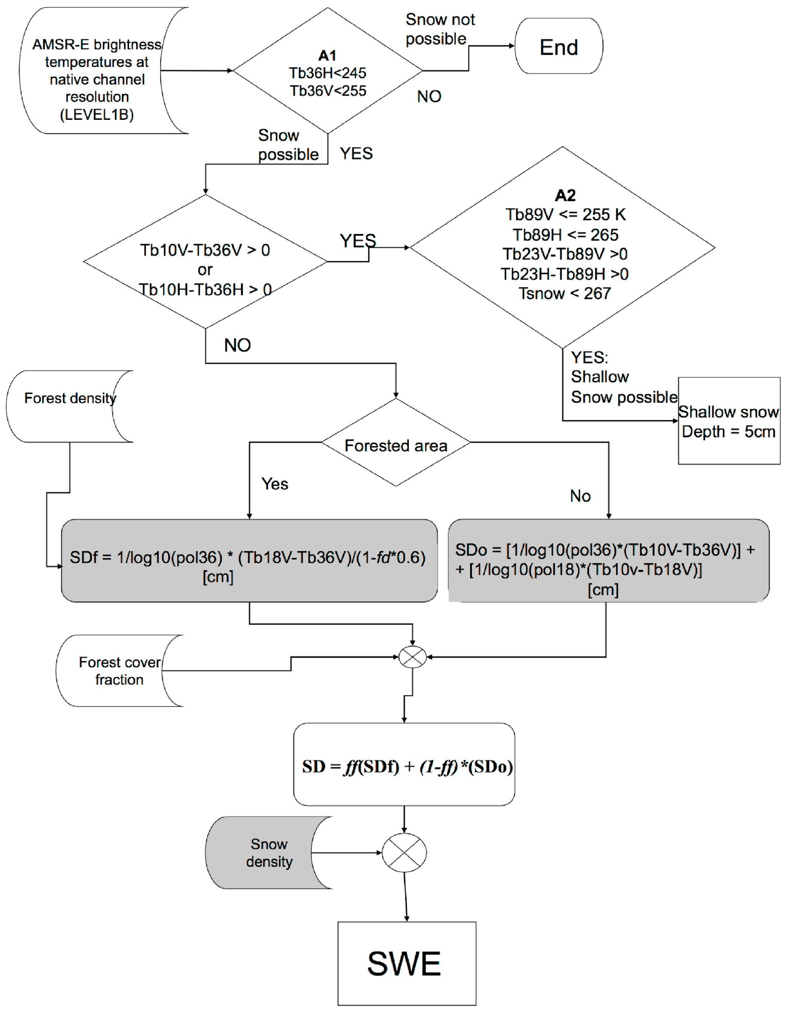
3.2. The New Operational Snow AMSR-E Algorithm

The new algorithm here proposed builds on the operational algorithm described in the previous section, addressing some of the issues identified in previous studies [53]. Major differences between the new and the existing algorithms consist in the way the retrieval coefficients relating passive microwave measurements to snow depth are computed, how the values of snow density used to convert snow depth to SWE are estimated and the use of ancillary datasets. In the new algorithm, indeed, the retrieval coefficients are computed using estimates of effective grain size obtained from artificial neural networks (ANNs) trained with the outputs of an electromagnetic model, specifically the Helsinki University of Technology electromagnetic model, TKK, formerly known as HUT [54]. In addition, the temporally static density map is replaced with a temporally and spatially varying dynamic map based on the work by Sturm et al. [17].

3.2.1. A New Scheme for Retrieval Coefficients

Grain size plays a dominant role in the retrieval of SWE and snow depth from spaceborne microwave brightness temperatures [48,53]. Because of the strong sensitivity of microwave brightness temperatures at the frequencies of interest to grain size, the knowledge of this parameter is crucial for constraining the inversion problem (e.g., estimates of snow parameters from a set of measured brightness temperatures). The current AMSR-E operational algorithm accounts for the grain size spatio-temporal variability by computing the retrieval coefficients from the polarization ratio of the recorded brightness temperatures. Nevertheless, previous studies have found a relatively weak correspondence between the retrieval coefficients estimated by the operational algorithm and the estimates of the microwave effective grain size obtained from the analysis of the outputs of an electromagnetic model [53]. This can lead to substantial error on snow depth/SWE estimates. For example, one of the reasons for overestimating snow depth from microwave data over specific regions in Eurasia is the underestimation of the effective grain size [24,41,55,56]. These studies show that the existence of strong temperature gradients between air surface and ground temperature over eastern Siberia tends to accelerate grain size metamorphism early in the season, thus increasing the size of effective microwave scatters early in the season. As an example, Figure 2 shows the average near-surface temperature for January 2006, derived from the combination of brightness temperatures and using the formula currently used in the AMSR-E operational algorithm (as given in Equation (16)). We observe that the near-surface temperatures are lower over the areas where the AMSR-E operational algorithm is overestimating snow depth [55], such as over Siberia. Despite the operational algorithm’s attempts to account for the grain size spatio-temporal variability (Equation (4) through Equation (9)), it is unable to account for the increase in the grain size due to the temperature gradient and the prediction of a smaller effective grain size with respect to the actual one produces higher snow depth values.

The retrieval coefficients in the current operational algorithm (Equations (6) and (7)) are replaced in the new algorithm here proposed with those in Equations (10) and (11):

$$newfac{t}_{36}= \frac{pfros{t}_{fact}}{\exp \left(g{r}_{36}-g{r}_0\right)}$$

(10)

$$newfac{t}_{18\_36}= \frac{pfros{t}_{fact}}{\exp \left(g{r}_{18\_36}-g{r}_0\right)}$$

(11)

where

$$pfros{t}_{fact}= \frac{pfros{t}_{clim\_temp}}{240}$$

(12)

$$pfros{t}_{clim\_temp}= \frac{V_{10GHz\_clim}}{0.95}$$

(13)

and gr₃₆ and gr_{18_36} are the grain size estimated using only the 36.5 GHz brightness temperatures or both the 18.7 and 36.5 GHz values, respectively. The idea behind these coefficients is to use grain size estimates from the inversion of an electromagnetic model and account for this through the exponential function in the formula. The reason for selecting two different grain size values is to account for the different penetration depths of the microwave frequencies within the snowpack and the vertical distribution. The value of gr₀ in Equations (10) and (11) was estimated as the grain size value that would correspond to the effective grain size used in the current operational algorithm when using the formula for the new coefficients, and was found to be 0.9 mm. The pfrostfact term aims at accounting for the distribution of permafrost underlying the snowpack, which impacts both the grain size metamorphism and the brightness temperatures at the lower frequencies (e.g., ~10 and ~19 GHz). The permafrost maps are obtained from [57] (updated 2001). For practical purposes, pfrostfac is set to 1 if it exceeds the value of 1. In the formula, V10 GHz_clim is the C-band vertical polarization brightness temperature climatology (2002–2009). The value of 240 K was derived from the analysis of the brightness temperatures over permafrost areas. Specifically, this value was obtained as the mean brightness temperature at 10 GHz for the months of November and December for those regions where permafrost is existing according to [57]. The value of 0.95 to obtain estimates of the permafrost temperature from the brightness temperatures at ~10 GHz was derived following Zuerndorfer et al. [58].

The values of gr₃₆ and gr_{18_36} are obtained from the minimization of the difference between measured (AMSR-E) and simulated brightness temperatures. For computational efficiency, the minimization procedure is carried out by means of artificial neural networks (ANNs). ANNs consist of interconnected neurons that exchange messages between each other. The connections have numeric weights that are tuned based on inputs–outputs datasets (called training dataset), allowing them to learn the relationship between inputs and outputs. ANNs can be seen as multivariate, non-linear approximations of the relationship between brightness temperature inputs and grain size outputs [20]. In the ANN, the input layer is passed through many hidden layers (made of certain number of neurons) [59]. The output O of the ANN can be expressed in terms of matrix algebra as:

$$O=LW \times tansig\left(IW \times I+B_0\right)+ B_1$$

(14)

where IW is the input weight matrix, LW is the layer weight matrix and B₀ and B₁ are bias vectors corresponding to the trained ANN. I is the input vector made of the brightness temperature values and tansig is a sigmoidal function defined as:

$$tansig\left(x\right) = \frac{2}{\left(1+exp\left(-2x\right)\right)}-1$$

(15)

The ANN here used is a feed forward network [59] with one hidden layer containing four neurons. This optimal ANN architecture is chosen by comparing the performance of different architectures using the root mean square error (RMSE) between measured and estimated surface brightness temperatures at 18.7 and 36.5 GHz, both horizontal and vertical polarization, as a metric. Training is performed through a back propagation algorithm [20,59]. The training dataset is here obtained using the inputs and outputs of the TKK electromagnetic model [22] and consists of simulated brightness temperatures and the corresponding snow depth, density and temperature inputs (

Table 3. Range of the snow parameters used as inputs to the electromagnetic model to generate the set of simulated brightness temperatures used to train the artificial neural network.

Snow Parameter	Minimum	Maximum	Step
Snow Temperature (°C)	−30	0	2.5
Snow depth (m)	0	1	0.1
Snow density (g/cm3)	0.1	0.4	0.025
Grain size (mm)	0.1	1.6	0.1

). The only output of the ANN consists of the grain size. Two separate ANNs are trained for the estimation of the gr₃₆ and gr_{18_36} values: a first one accepting only the 36.5 GHz Tb values as input and a second one using both the 18.7 and 36.5 GHz Tb values. Once trained, the ANN can be interrogated to provide estimates of the effective grain size. To this aim, values of measured brightness temperatures, snow depth, density and temperature need to be provided to the trained ANN. In this case, snow depth consists of the snow depth monthly climatology values where density is obtained following the approach in [17], using the monthly snow depth climatology values, the day of the year and snow classes as inputs. Near-surface temperatures are obtained from the same approach adopted in the current operational algorithm. We point out that the goal of this activity is to identify the values for the effective grain size characterizing the snowpack under observation. As an example, Figure 3 shows a map of effective grain size estimated from the ANN (using only the 36.5 GHz brightness temperatures) on 1 January 2004. The figure clearly shows the larger values over Siberia captured in our approach, where the operational algorithm generally overestimates snow depth. As we will see in Section 4, the larger effective grain size values here are considerably improving estimates of snow depth over that region.

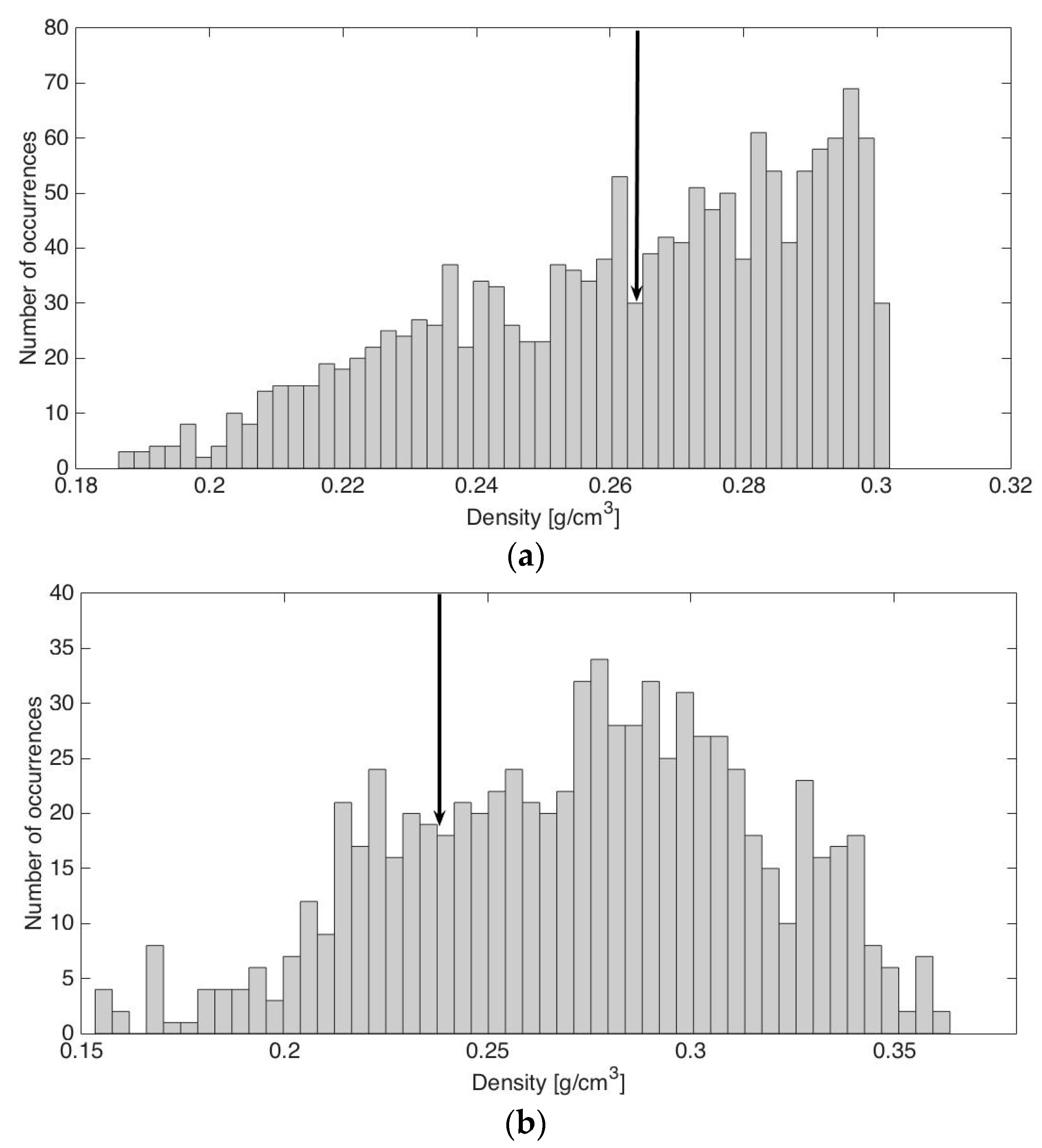
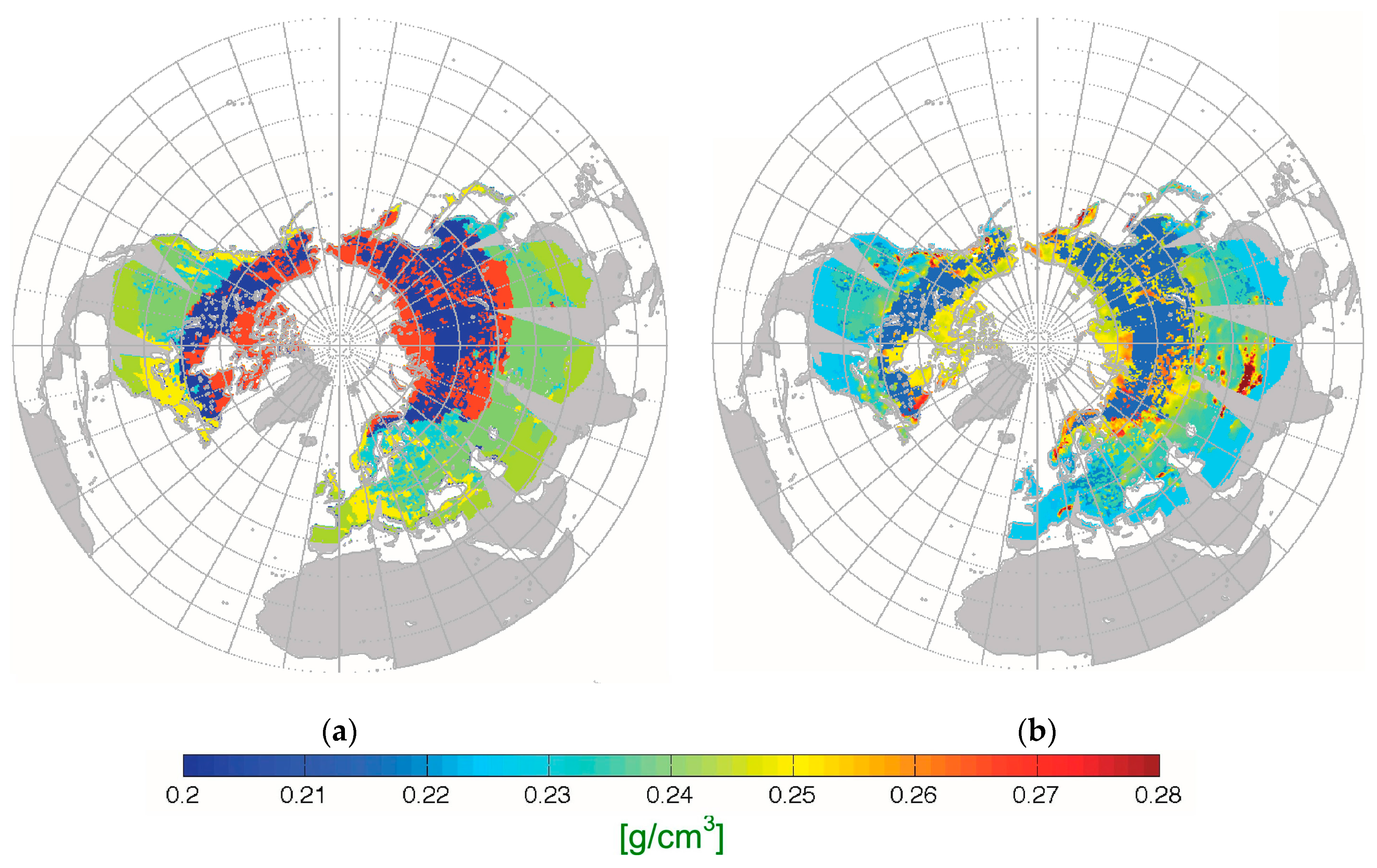
3.2.2. Snow Temperature and Snow Density

In the operational AMSR-E SWE algorithm, near-surface temperature (Ts, in °C) is estimated from the linear combination of measured brightness temperatures [25]

$$T_s=58.08-0.39T{b}_{19V}+1.21T{b}_{23V}-0.37T{b}_{37H}+0.36T{b}_{89V}-273.15$$

(16)

In the algorithm here proposed, similar to the approach proposed to estimate the effective grain size, the linear regression in Equation (16) is replaced with a non-linear multivariate regression approach based on ANNs. The ANN is driven with brightness temperatures measured at K and Ka bands, (both vertical and horizontal polarization), the 22.7 GHz brightness temperature (vertical polarization) and the 89 GHz brightness temperatures. A database containing ~630,000 values of co-registered WMO station data and AMSR-E brightness temperatures [60] was divided into three subsets that were used to train and evaluate the performance of the ANN [20]. The average RMSE between ANN-estimated and measured near-surface temperatures is 6.8 °C, with mean absolute error (MAE) of 5.55 °C, an improvement with respect to the values obtained with the linear regression formula (RMSE of 8.82 °C and MAE of 6.54 °C). The linear regression coefficient between estimated and measured surface temperature is R = 1.06 in the case of the ANN and R = 1.13 in the case of the linear formula.

Estimates of snow density are used to convert snow depth obtained from spaceborne brightness temperatures to SWE. As mentioned above, in the operational version of the current AMSR-E SWE algorithm, a temporally static mask of snow density values is used for this purpose. Despite the fact that the density map is spatially variable, no spatial variability occurs within each snow class. Still, density does evolve during the snow season and within each snow class. It is therefore important to account for this process to potentially improve SWE estimates [53]. In the new algorithm, daily snow density maps are obtained following the formulas reported in [17]. Here, a statistical model based on a Bayesian analysis of a set of 25,688 depth-density-SWE data collected in the U.S., Canada, and Switzerland uses snow depth (SD), day of the year (DOY), and the climate class of snow (SC) to produce estimates of a local bulk density. In the version adopted in our algorithm, for operational purposes, daily snow depth values are replaced with values of monthly snow depth climatology. The bulk density for each pixel and day is, therefore, obtained as follows:

$$\rho \left(DOY, SD, SC\right)=\left({\rho }_{max}-{\rho }_0\right)\left(1-\exp \left(-k_1\ast D-k_2\ast DOY\right)\right)+{\rho }_0$$

(17)

where DOY is the day of the hydrological year (running from Day −92 for 1 October to Day 181 for 30 June) and ρ_max, ρ₀, k₁ and k₂ are coefficients that vary with snow class. These values are reported for reader’s convenience in Table S1 for the different snow classes [17]. In Sturm et al. [17], the parameters for the snow class denoted as Ephemeral are not computed. The density value for those pixels where ephemeral snow is present is, therefore, set to the static value of 0.2275 g/cm³. This aspect should be addressed in future algorithms refinements. Examples of snow density maps used in the operational algorithm and in the one here proposed are reported in Figure 4. Because both approaches make use of snow classes identified in Liston and Sturm [61], the spatial patterns of density are similar. Additionally, Figure 5 shows the distribution of density as computed with the new AMSR-E algorithm for all months and years for a pixel belonging to the (Figure 5a) maritime and (Figure 5b) prairie classes. Black arrows indicate the density values used in the case of the static previous algorithm. The differences that exist between the two maps are due to the dependency of snow density values computed in the new algorithm on snow depth. As mentioned in Sturm et al. [17], the approach here used to calculate the bulk density from DOY, SD and snow classes is particularly applicable for operational purposes. The good performance of the method found in Sturm et al. [17] is due to the existence of a statistical relationship between bulk density and snow depth, time of year, and climate class of snow and because snow density is a conservative variable that in nature is constrained between fairly narrow limits.

3.3. Validation Datasets

3.3.1. Canadian Meteorological Centre Dataset

The Canadian Meteorological Centre (CMC) dataset for the northern hemisphere [62] includes daily observations from 1998 to 2013 and monthly averages of SWE and snow depth. The CMC product is generated from the combination of snow depth data obtained from surface synoptic observations, meteorological aviation reports and special aviation reports from the World Meteorological Organization (WMO [63] by interpolating such observations using a more sophisticated approach in which other components (beside the ground observations) are used to generate maps from point scale measurements. First, real-time snow depth data are acquired from the WMO information system. The analysis is updated every six hours using optimum interpolation, with the initial value provided by a simple snow accumulation and melt model using analyzed temperatures and forecast precipitation from the CMC Global Environmental Multiscale (GEM) forecast model [64]. In those regions where there are no observations of snow depth, the snow depth shown in the analysis corresponds to the initial guess field simplified assumptions regarding snowfall, melt and aging.

A complete description of the analysis methodology and validation is published in previous studies [62,65]. Because over most of the Arctic region there are no observations, the analysis is based on estimated snow depths from the first guess field. Moreover, snow depth observations over northern Canada might be biased to coastal locations with observing sites at open areas near airports.

3.3.2. WMO Ground Observations Co-Registered with AMSR-E Data

We also use spatially and temporally AMSR-E co-registered WMO observations provided by the NSIDC [60]. The temporal coverage of this data set spans from 1 January 2002 through 19 March 2009. Documentation for this dataset is available at [66]. The distribution of WMO stations used for the assessment of the AMSR-E product is reported in Figure 6.

3.3.3. The GlobSnow Product

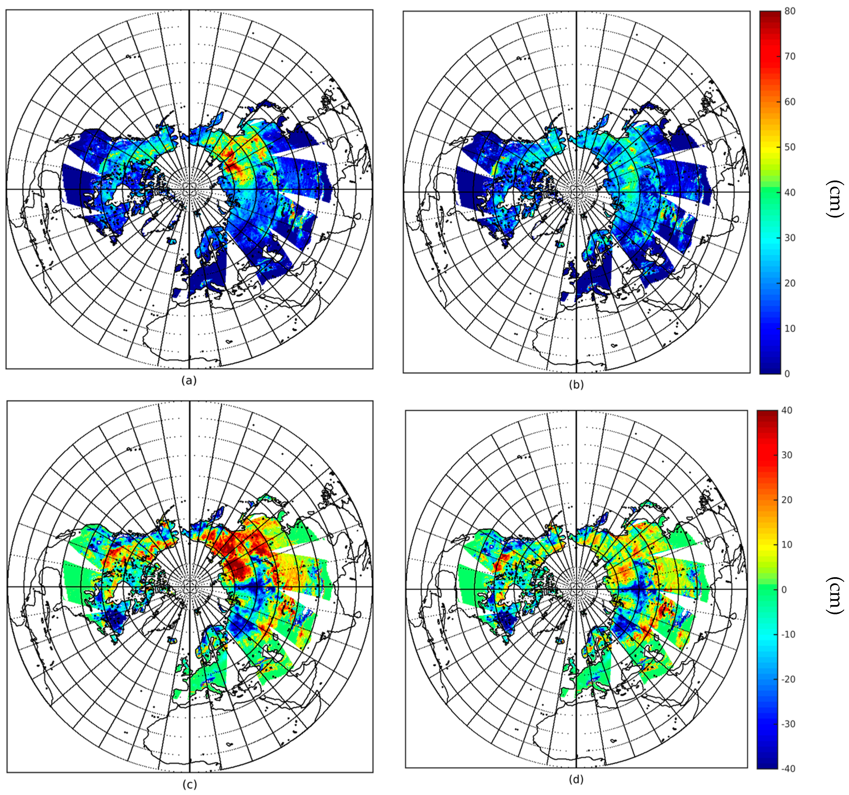
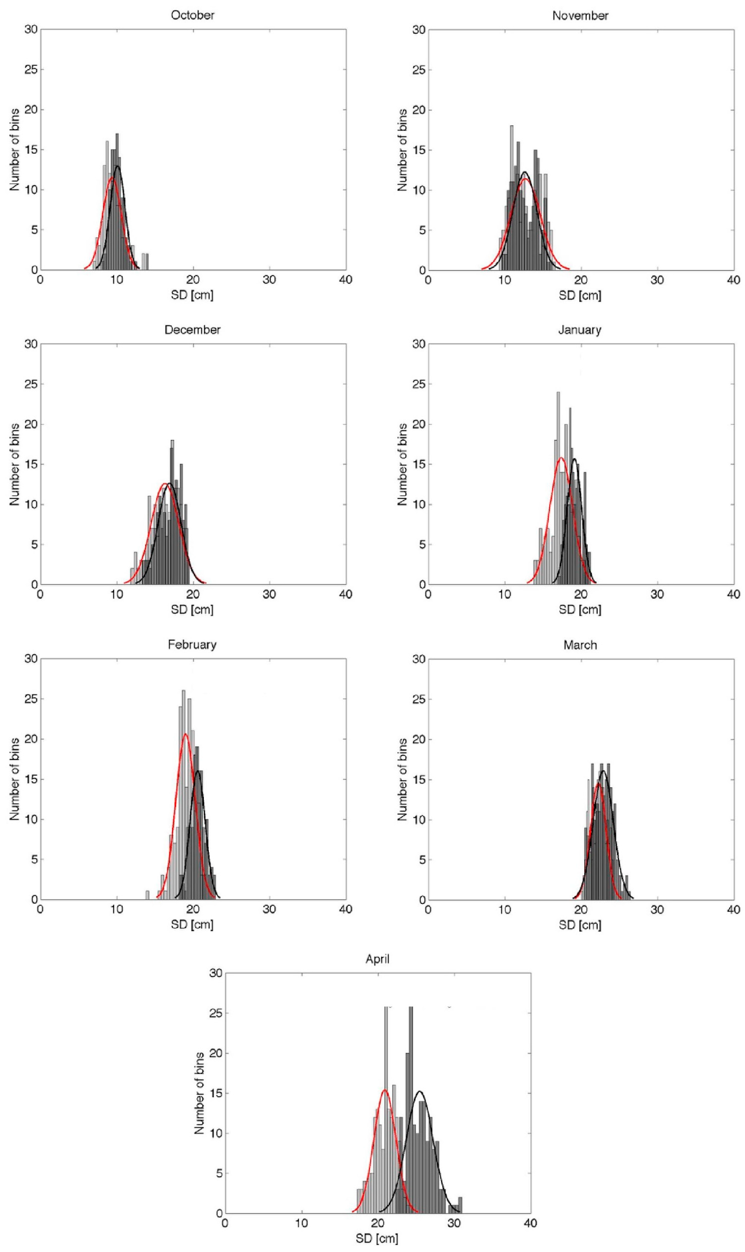
The GlobSnow product has been generating global gridded information on snow extent and SWE across the Northern Hemisphere combining information from spaceborne microwave radiometers and ground-based weather stations [67]. The approach used in GlobSnow is similar to the one proposed in the new algorithm, making use of the same frequencies (with the exception of the 10 GHz). In GlobSnow, however, the inversion of the electromagnetic model is obtained through an iterative minimization procedure. Still, the major difference consists in the snow depth ancillary information used in the algorithm. In GlobSnow, daily snow depth background fields are generated from observations at synoptic weather stations acquired from European Centre for Medium-Range Weather Forecasts (ECMWF) for the years 1979 to present. The ECMWF snow depth data were enhanced with the inclusion of the INTAS-SCCONE (International Association for the promotion of co-operation with scientists from the New Independent States of the former Soviet Union—Snow Cover Changes Over Northern Eurasia) snow depth dataset [68]. The synoptic weather station data set is first filtered from extremely large snow depth values (over 300 cm, typically occurring only in mountains or extreme locations) and then a median filter is applied to remove values that differ more than 50 cm from the median of 11 days’ time frame for each station. Stations with at least 20 measurements for at least five separate years are kept while the remaining stations are removed. Stations with unusually deep snow conditions (e.g., mean of March over 150 cm) are also filtered out if the deep snow conditions have occurred at least 50% of the years that the station has had at least 20 measurements. Differently from the approach used in our new algorithm (based on ANN), the methodology for SWE retrieval employed by GlobSnow utilizes a Bayesian non-linear iterative assimilation approach first described in Pulliainen [22] and complemented in Takala et al. [23]. The available synoptic weather station measurements of snow depth are used as input to the HUT snow emission model ([28,54]), describing the scene brightness temperature as a function of the characteristics of the snowpack (depth, bulk density and grain size) and forest canopy (stem volume/biomass). Snow parameters are then extracted by minimizing the difference between measured and simulated brightness temperatures [22]. Density used to convert snow depth to SWE is kept fixed at 0.248 g/cm³. This is also another difference between GlobSnow and our algorithm. Lastly, mountain regions are excluded from GlobSnow. Within GlobSnow, an EASE-Grid cell is considered as mountainous if the standard deviation of the elevation within a grid cell is above 200 m [67].

4. Results

4.1. Comparison between AMSR-E and CMC

Table 4. Monthly averaged correlation values, Root Mean Squared Error (RMSE), slope and bias between the AMSR-E derived snow depth values and those estimated in the Canadian Meteorological Centre (CMC) data set.

	AMSR-E Operational			New Algorithm
	Correlation	RMSE (cm)	Bias (cm)	Correlation	RMSE (cm)	Bias (cm)
October	0.20	7.24	3.94	0.48	6.80	0.56
November	0.28	13.03	7.90	0.50	10.97	2.43
December	0.23	19.97	13.48	0.55	14.88	3.55
January	0.31	28.03	13.59	0.40	25.70	10.33
February	0.40	30.88	11.36	0.49	28.00	7.90
March	0.38	34.94	12.11	0.43	32.73	10.17
April	0.42	24.51	5.03	0.45	25.23	4.22

shows the correlation (R²), RMSE and bias between AMSR-E derived snow depth values and those obtained with the CMC product for the months of October through April. Only snow depth values below 80 cm in the CMC product were used for the results reported in the table, in order to account for the saturation effect discussed in Section 2. The value was selected based on the threshold currently used in the operational algorithm. The table clearly indicates that the new algorithm performs better than the operational one (when CMC is used as a validation data set) for all months. In our analysis, we did not report the values for the months of May through September as the snow cover extent is relatively small and snow is present mostly over the Arctic region for that period. The improvement of the new algorithm with respect to the operational one is strongly driven by the use of the a-priori knowledge on grain size. As an example, Figure 7 shows snow depth values obtained with (Figure 7a) the operational AMSR-E SWE algorithm, (Figure 7b) the algorithm here proposed, the differences between (Figure 7c) the operational and CMC, and (Figure 7d) the new and CMC for 1 January 2004. Again, we note that the new algorithm performs considerably better than the current algorithm especially over Siberia (where, as we mentioned, large effective grains not captured by the operational algorithm are responsible for the overestimation of snow depth). Over the remaining regions, the new algorithm does not introduce a considerable bias or considerable changes over those areas where the operational algorithm is already performing relatively well. We also studied the performance of the operational and new algorithms with respect to forest cover fraction. Our results, reported in Tables S2 through S7, confirm that the new algorithm performs better than the existing one for all forest density ranges. We suggest this might be due to the improvement introduced in the new algorithm associated with the grain size spatio-temporal variability, which also accounts for the impact of vegetation on snow parameters. However, a more detailed analysis, which is beyond the scope of this paper, is required to better understand the reasons for the improved performance with respect to forest density of the new algorithm.

4.2. Comparison of Spaceborne Estimates with WMO Data

The results of the comparison between AMSR-E and WMO snow depth values are reported in

Table 5. RMSE, Slope and bias of the AMSR-E estimated and WMO measured snow depth values using the original and the modified algorithm.

	Operational			New Algorithm
	Correlation	RMSE (cm)	Bias (cm)	Correlation	RMSE (cm)	Bias (cm)
October	0.12	11.43	11.23	0.18	10.35	10.24
November	0.21	13.65	13.82	0.29	13.16	11.02
December	0.32	17.15	18.21	0.39	16.13	13.58
January	0.36	20.66	29.19	0.42	17.39	20.57
February	0.22	22.78	37.88	0.21	19.17	27.54
March	0.14	27.34	45.62	0.13	24.70	37.29
April	0.11	32.12	44.68	0.12	27.90	30.30

. One limitation in this case consists in the point-scale nature of the WMO measurements with respect to the large-scale nature of the AMSR-E observations. This is an important issue and, unfortunately, can be solved only by increasing the number of observations within each pixel, as suggested in [47]. For each day, an average number of 2000 stations is used to evaluate the results of the remote sensing algorithms. The number of stations used varies on a daily basis, depending on the maximum snow depth and near-surface temperatures. Besides excluding snow depth measurements that exceed 80 cm, we also excluded those days when near-surface temperature is above 0 °C, to reduce the probability of wet snow occurrence. The map of the distribution of the WMO stations (Figure 3) shows that many stations are located in Europe and a relatively low number of stations are located in Eurasia and North America. In addition, WMO stations poorly cover Eastern Siberia, suggesting that an improvement is also obtained over areas other than Siberia.

4.3. Comparison of Spaceborne Estimates with GlobSnow

4.3.1. Snow Depth

Figure 8 shows the histograms of the difference between GlobSnow snow depth values and those estimated from AMSR-E using the two algorithms considered in this study. In the figure, the light grey bars and red curve correspond to the new algorithm here proposed, while the dark bars and the black curve correspond to the operational algorithm. The histograms of the differences are fitted with Gaussian distributions and the values for the mean and standard deviation obtained from the fitting are reported in Table S8. Overall, the new algorithm performs generally better than the operational one with the differences increasing from October through April. This might be due to a combination of factors, such as the saturation effect described above, the vertical distribution of snow grain size and density as well as the presence of ice lenses or layers within the snowpack. We speculate that these factors might be captured by the GlobSnow product in view of its ingestion of in-situ measurements, but are missed by the AMSR-E algorithms. The values of the mean in the case of the two algorithms are similar for the months of October, November, December and March, with the new algorithm generally providing a smaller mean (e.g., better matching with GlobSnow) than the operational algorithm (Table S8). For the remaining months, the new AMSR-E algorithm provides a better agreement with the GlobSnow product, with the largest difference in April (~5 cm, equivalent to ~25% of the AMSR-E operational product mean difference), followed by January (~1.8 cm, ~10%) and February (1.58 cm, ~10%).

Table 6. Monthly averaged correlation values, RMSE, slope and bias between the AMSR-E derived snow depth values and those estimated in the GlobSnow data set.

	AMSR-E Operational			New Algorithm
	Correlation	RMSE (cm)	Bias (cm)	Correlation	RMSE (cm)	Bias (cm)
October	0.41	9.87	2.56	0.47	8.56	1.40
November	0.39	11.2	6.67	0.45	9.87	4.12
December	0.41	14.32	11.38	0.51	12.43	4.34
January	0.32	26.45	11.89	0.47	17.89	8.72
February	0.43	33.76	14.55	0.42	21.54	8.97
March	0.37	38.67	13.12	0.39	24.43	12.63
April	0.21	22.31	5.19	0.32	18.73	4.12

provides also the metrics between AMSR-E products and GlobSnow as reported in the previous sections, including correlation, RMSE and bias. The standard deviation in the case of the new algorithm is generally larger than the one obtained when considering the operational algorithm. It is not clear why this is happening, but we plan to further look into this for improving the performance of the new algorithm. We remind here that both the new AMSR-E algorithm here proposed and GlobSnow make use of a-priori information on snow depth and this might be a driving factor for the improved performance of the new AMSR-E algorithm with respect to the operational one.

4.3.2. SWE

The unavailability of spatially dense measurements of SWE on ground is a limiting factor for the assessment and the evaluation of the SWE estimated from AMSR-E. When available, indeed, SWE measurements are not performed systematically or continuously over time, with those few measurements carried out at automatic stations being mainly located at high elevations, where they are not representative of the large area observed by the passive microwave sensor and where forest fraction can be very high. One way to circumvent this problem consists in comparing the outputs of the AMSR-E algorithm with other remote sensing and global snow products. This can offer a tool to understand issues and problems related to the products under consideration. As in the previous section, therefore, we compared the SWE estimated from AMSR-E from the two algorithms with SWE estimates from the GlobSnow product. As in Figure 8, Figure 9 shows the histograms of the difference between GlobSnow and AMSR-E SWE estimates obtained using the new and operational algorithms. The values of the means and standard deviations of the Gaussian distributions fitting the differences are reported in Table S9. Correlation, RMSE and bias are reported in

Table 7. Monthly averaged correlation values, RMSE, slope and bias between the AMSR-E derived SWE values and those estimated in the GlobSnow data set.

	AMSR-E SWE Operational			New SWE Algorithm
	Correlation	RMSE (mm)	Bias (mm)	Correlation	RMSE (mm)	Bias (mm)
October	0.33	17.14	8.74	0.43	16.70	6.76
November	0.32	22.15	11.43	0.35	19.58	8.37
December	0.29	25.67	18.87	0.38	19.29	13.25
January	0.28	34.63	22.78	0.39	27.33	31.09
February	0.41	40.17	19.23	0.40	32.34	18.67
March	0.38	46.56	21.39	0.39	35.68	17.23
April	0.13	37.87	18.11	0.22	29.21	14.30

. Similarly to snow depth, the new AMSR-E algorithm generally matches better the GlobSnow values than the operational one, with the exception of the months of November and March. One factor that needs to be accounted for when comparing SWE estimates from the different approaches is that the GlobSnow product uses a fixed density value (0.24 g/cm³) to convert snow depth estimates into SWE, whereas the operational AMSR-E algorithm uses a spatially dynamic, but temporally static density map, and the new algorithm uses a spatio-temporally dynamic map. This, obviously, makes the assessment of the comparison of the SWE values obtained with the three algorithms more difficult as it does not allow to properly understand whether the improvement (or deterioration) of one algorithm vs. another is due to snow depth or to the different use of density values used to extract SWE. In this regard, parallel activities with European and Canadian colleagues are ongoing [69].

Despite the prototype algorithm producing improved estimates of SWE, there are still several issues that remain to be addressed for improving SWE estimates from spaceborne passive microwave data. Building on previous studies [45], we are evaluating an optimal way of performing operational atmospheric correction to the measured brightness temperatures, in order to reduce the uncertainty on SWE retrieval. Improvements are also being sought in the case of forest. Several approaches different from the one currently used will be evaluated to account for the “masking” effect due to vegetation. Other data sets will also be considered and the combined use of forest fraction and forest density (proposed in the current algorithm, but here not considered) will also be re-evaluated.

5. Conclusions

Building on the current AMSR-E SWE operational algorithm, we have implemented and assessed a new algorithm for estimating SWE and snow depth from historical AMSR-E brightness temperatures. The main differences between the algorithm here proposed and the current operational AMSR-E SWE one consist in: (1) the use of artificial neural networks in combination with an electromagnetic model to estimate effective grain size. This, in turn, is used to compute the retrieval coefficients relating brightness temperature differences (at different frequencies) to snow depth; (2) density values that are used to convert snow depth to SWE are spatially and temporally dynamically computed, replacing the previous temporally static map of density values used in the operational algorithm; (3) estimates of near-surface snow temperature are performed using artificial neural networks, rather than using a linear regression approach as in the current operational algorithm. The new algorithm also generates maps of snow bulk density and effective grain size that can be, eventually, of benefit for the scientific community.

The comparison between the results obtained with the AMSR-E SWE algorithm here proposed and several independent data sets shows that the new algorithm performs better than the operational one, especially over those areas where large snow grains can be present. Though there has been small or no analysis concerning the use of maps of effective grain size, the availability of such parameter as part of an operational product would offer the possibility to perform new investigations. For example, the effective grain size could be related to the snow age or to support a better understanding on when saturation effects occur due to the impact of snow grains on brightness temperature at low frequencies.

Differently from the operational one, the new algorithm makes use of a-priori information (snow depth climatology in this case) to increase the probability that the effective grain size value used for the retrieval is close to what would be expected given the snow climatic conditions of the area. This action is undertaken to minimize the impact of the ill-posed nature of the retrieval problem. A similar approach has been used by the European and Canadian agencies to produce an operational SWE retrieval (GlobSnow, www.globsnow.info). Differences between the GlobSnow algorithm and the one here proposed consist in the use of climatological information (our algorithm) rather than daily measured values from ground stations (GlobSnow) and the use of ANN for the inversion procedure. Moreover, the current version of GlobSnow uses a fixed density of 0.248 g/cm³ for converting snow depth to SWE, while in our case a dynamic map is used (though plans for GlobSnow2 are to use the same approach adopted in our algorithm, Chris Derksen, Pers. Comm.). The reason for using snow depth monthly climatologies rather than daily information as in the case of GlobSnow is related to the choice for our algorithm to be self-consistent, meaning that all the data required for the SWE estimate is measured by the AMSR-E sensor itself or it is available as ancillary datasets. The possibility of using external, near-real-time datasets is currently under study for the AMSR2 operational SWE product.

Despite the prototype algorithm producing improved estimates of SWE, there are still several issues that remain to be addressed for improving SWE estimates from spaceborne passive microwave data. Building on previous studies [45], we are evaluating an optimal way of performing operational atmospheric correction to the measured brightness temperatures, in order to reduce the uncertainty on SWE retrieval. Improvements are also being sought in the case of forest. Several approaches different from the one currently used will be evaluated to account for the ‘masking’ effect due to vegetation. Other data sets will also be considered and the combined use of forest fraction and forest density (proposed in the current algorithm, but here not considered) will also be re-evaluated.

The retrieval of snow depth and SWE at large spatial scales from spaceborne passive microwave data remains one of the key aspects for quantifying the long-term changes and trends of snow mass at global scale with a high temporal resolution. Regardless of whether focusing on the improvement of pure remote sensing algorithms or on the combination of remote sensing retrieval schemes supported by other tools, such as data assimilation or ancillary information, it is crucial to continue improving our skills in estimating both snow depth and SWE from the available datasets. This will support not only the re-analysis of historical datasets, but it will lay the ground for future improved operational algorithms, reducing the uncertainty on estimates of snow depth and SWE that can span for more than 35 years. In this regard, our study shows that large improvements can be made by including knowledge of physical processes into remote sensing retrieval schemes. This, in conjunction with ancillary data, represents a powerful tool to overcome some of the known issues limiting the improvement of the algorithms solely based on remote sensing data. Our plan is to continue improving the retrieval scheme here proposed and extend its application to both AMSR2 and SSMI and complement the ongoing efforts on ground and from the climate modeling community to build a more robust and improved time series of the changes occurring to the snow on our planet.

References

1. Zhang, X.; Zwiers, F.W.; Hegerl, G.C.; Lambert, F.H.; Gillett, N.P.; Solomon, S.; Stott, P.A.; Nozawa, T. Detection of human influence on twentieth-century precipitation trends. Nature 2007, 448, 461–465. [Google Scholar] [CrossRef] [PubMed]
2. Cohen, J. Snow cover and climate. Weather 1994, 49, 150–156. [Google Scholar] [CrossRef]
3. Mote, T.L. On the role of snow cover in depressing air temperature. J. Appl. Meteorol. Climatol. 2008, 47, 2008–2022. [Google Scholar] [CrossRef]
4. Graybeal, D.Y.; Leathers, D.J. Snowmelt-related flood risk in Appalachia: First estimates from a historical snow climatology. J. Appl. Meteorol. Climatol. 2006, 45, 178–193. [Google Scholar] [CrossRef]
5. Leathers, D.J.; Robinson, D.A. The association between extremes in North American snow cover extent and United States temperatures. J. Clim. 1993, 6, 1345–1355. [Google Scholar] [CrossRef]
6. Jones, H.G.; Pomeroy, J.W.; Walker, D.A.; Hoham, R.W. (Eds.) Snow Ecology: An Interdisciplinary Examination of Snow-Covered Ecosystems, 1st ed.; Cambridge University Press: Cambridge, UK; New York, NY, USA, 2001.
7. Barnett, T.P.; Adam, J.C.; Lettenmaier, D.P. Potential impacts of a warming climate on water availability in snow-dominated regions. Nature 2005, 438, 303–309. [Google Scholar] [CrossRef] [PubMed]
8. Barry, R.G. The role of snow and ice in the global climate system: A review. Polar Geogr. 2002, 26, 235–246. [Google Scholar] [CrossRef]
9. Armstrong, R.; Knowles, K.; Brodzik, M.; Hardman, M.A. DMSP SSM/I-SSMIS Pathfinder Daily EASE-Grid Brightness Temperatures, version 2; NASA National Snow Ice Data Center Distributed Active Archive Center: Boulder, CO, USA, 1994. [Google Scholar]
10. Knowles, K.E.; Njoku, G.; Armstrong, R.; Brodzik, M. Nimbus-7 SMMR Pathfinder Daily EASE-Grid Brightness Temperatures, version 1; NASA National Snow Ice Data Center Distributed Active Archive Center: Boulder, CO, USA, 2000. [Google Scholar]
11. Ulaby, F.T.; Moore, R.K.; Fung, A.K. Microwave Remote Sensing: Active and Passive, Volume 1—Microwave Remote Sensing Fundamentals and Radiometry; Microwave Remote Sensing; Artech House Publishers: Norwood, MA, USA, 1981; Volume 1, p. 456. [Google Scholar]
12. Aschbacher, J. Land Surface Studies and Atmospheric Effects by Satellite Microwave Radiometry. Ph.D. Thesis, University of Innsbruck, Innsbruck, Austria, 1989. [Google Scholar]
13. Chang, A.; Foster, J.L.; Hall, D.K. Nimbus-7 SMMR derived monthly global snow cover and snow depth. Ann. Glaciol. 1987, 9, 39–44. [Google Scholar]
14. Foster, J.L.; Chang, A.T.C.; Hall, D.K. Comparison of snow mass estimates from a prototype passive microwave snow algorithm, a revised algorithm and a snow depth climatology. Remote Sens. Environ. 1997, 62, 132–142. [Google Scholar] [CrossRef]
15. Hallikainen, M.T.; Jolma, P.A. Comparison of algorithms for retrieval of snow water equivalent from Nimbus-7 SMMR data in Finland. IEEE Trans. Geosci. Remote Sens. 1992, 30, 124–131. [Google Scholar] [CrossRef]
16. Tait, A. Estimation of snow water equivalent using passive microwave radiation data. In Proceedings of the 1996 International Geoscience and Remote Sensing Symposium—Remote Sensing for a Sustainable Future, Lincoln, NE, USA, 27–31 May 1996.
17. Sturm, M.; Taras, B.; Liston, G.E.; Derksen, C.; Jonas, T.; Lea, J. Estimating snow water equivalent using snow depth data and climate classes. J. Hydrometeorol. 2010, 11, 1380–1394. [Google Scholar] [CrossRef]
18. Derksen, C.; Toose, P.; Rees, A.; Wang, L.; English, M.; Walker, A.; Sturm, M. Development of a tundra-specific snow water equivalent retrieval algorithm for satellite passive microwave data. Remote Sens. Environ. 2010, 114, 1699–1709. [Google Scholar] [CrossRef]
19. Clifford, D. Global estimates of snow water equivalent from passive microwave instruments: History, challenges and future developments. Int. J. Remote Sens. 2010, 31, 3707–3726. [Google Scholar] [CrossRef]
20. Tedesco, M.; Pulliainen, J.; Takala, M.; Hallikainen, M.; Pampaloni, P. Artificial neural network-based techniques for the retrieval of SWE and snow depth from SSM/I data. Remote Sens. Environ. 2004, 90, 76–85. [Google Scholar] [CrossRef]
21. Tedesco, M.; Kim, E.J. Intercomparison of electromagnetic models for passive microwave remote sensing of snow. IEEE Trans. Geosci. Remote Sens. 2006, 44, 2654–2666. [Google Scholar] [CrossRef]
22. Pulliainen, J. Mapping of snow water equivalent and snow depth in boreal and sub-arctic zones by assimilating space-borne microwave radiometer data and ground-based observations. Remote Sens. Environ. 2006, 101, 257–269. [Google Scholar] [CrossRef]
23. Takala, M.; Luojus, K.; Pulliainen, J.; Derksen, C.; Lemmetyinen, J.; Kärnä, J.P.; Koskinen, J.; Bojkov, B. Estimating northern hemisphere snow water equivalent for climate research through assimilation of space-borne radiometer data and ground-based measurements. Remote Sens. Environ. 2011, 115, 3517–3529. [Google Scholar] [CrossRef]
24. Grippa, M.; Kergoat, L.; Le Toan, T.; Mognard, N.M.; Delbart, N.; L’Hermitte, J.; Vicente-Serrano, S.M. The impact of snow depth and snowmelt on the vegetation variability over central Siberia. Geophys. Res. Lett. 2005, 32. [Google Scholar] [CrossRef]
25. Kelly, R.E.; Chang, A.T.; Tsang, L.; Foster, J.L. A prototype AMSR-E global snow area and snow depth algorithm. IEEE Trans. Geosci. Remote Sens. 2003, 41, 230–242. [Google Scholar] [CrossRef]
26. Tedesco, M.; Reichle, R.; Löw, A.; Markus, T.; Foster, J.L. Dynamic approaches for snow depth retrieval from spaceborne microwave brightness temperature. IEEE Trans. Geosci. Remote Sens. 2010, 48, 1955–1967. [Google Scholar] [CrossRef]
27. Fuller, M.C.; Derksen, C.; Yackel, J. Plot scale passive microwave measurements and modeling of layered snow using the multi-layered HUT model. Can. J. Remote Sens. 2015, 41, 219–231. [Google Scholar] [CrossRef]
28. Lemmetyinen, J.; Derksen, C.; Toose, P.; Proksch, M.; Pulliainen, J.; Kontu, A.; Rautiainen, K.; Seppänen, J.; Hallikainen, M. Simulating seasonally and spatially varying snow cover brightness temperature using HUT snow emission model and retrieval of a microwave effective grain size. Remote Sens. Environ. 2015, 156, 71–95. [Google Scholar] [CrossRef]
29. Che, T.; Li, X.; Jin, R.; Huang, C. Assimilating passive microwave remote sensing data into a land surface model to improve the estimation of snow depth. Remote Sens. Environ. 2014, 143, 54–63. [Google Scholar] [CrossRef]
30. De Lannoy, G.J.M.; Reichle, R.H.; Arsenault, K.R.; Houser, P.R.; Kumar, S.; Verhoest, N.E.C.; Pauwels, V.R.N. Multiscale assimilation of Advanced Microwave Scanning Radiometer–EOS snow water equivalent and Moderate Resolution Imaging Spectroradiometer snow cover fraction observations in northern Colorado. Water Resour. Res. 2012, 48. [Google Scholar] [CrossRef]
31. Tedesco, M.; Kelly, R.; Foster, J.L.; Chang, A.T.C. AMSR-E/Aqua Daily L3 Global Snow Water Equivalent EASE-Grids, version 2; NASA National Snow Ice Data Center Distributed Active Archive Center: Boulder, CO, USA, 2004. [Google Scholar]
32. AMSR-E Instrument Description. Available online: https://nsidc.org/data/docs/daac/amsre_instrument.gd.html (accessed on 13 October 2016).
33. Brodzik, M.J.; Knowles, K. EASE-Grid: A Versatile Set of Equal-Area Projections and Grids. In Discrete Global Grids; Goodchild, M., Ed.; National Center for Geographic Information & Analysis: Santa Barbara, CA, USA, 2002. [Google Scholar]
34. Tedesco, M.; Jeyaratnam, J.; Kelly, R. NRT AMSR2 Daily L3 Global Snow Water Equivalent EASE-Grids; NASA LANCE AMSR2 at the Global Hydrology Resource Center Distributed Active Archive Center: Huntsville, AL, USA, 2015. [Google Scholar]
35. Ulaby, F.T.; Moore, R.K.; Fung, A.K. Microwave Remote Sensing: Active and Passive; Artech House Publishers: Norwood, MA, USA, 1986. [Google Scholar]
36. Bernier, P.Y. Microwave remote sensing of snowpack properties: Potential and limitations. Hydrol. Res. 1987, 18, 1–20. [Google Scholar]
37. Mätzler, C. Applications of the interaction of microwaves with the natural snow cover. Remote Sens. 1987, 2. [Google Scholar] [CrossRef]
38. Tsang, L.; Kong, J.A. Scattering of electromagnetic waves from a dense medium consisting of correlated mie scatterers with size distributions and applications to dry snow. J. Electromagn. Waves Appl. 1992, 6, 265–286. [Google Scholar] [CrossRef]
39. Tsang, L.; Chen, C.T.; Chang, A.T.C.; Guo, J.; Ding, K.H. Dense media radiative transfer theory based on quasicrystalline approximation with applications to passive microwave remote sensing of snow. Radio Sci. 2000, 35, 731–749. [Google Scholar] [CrossRef]
40. Tsang, L.; Kong, J.A. Multiple scattering of electromagnetic waves by random distributions of discrete scatterers with coherent potential and quantum mechanical formalism. J. Appl. Phys. 1980, 51. [Google Scholar] [CrossRef]
41. Zurk, L.M.; Ding, K.H.; Tsang, L.; Winebrenner, D.P. Monte Carlo simulations of the extinction rate of densely packed spheres with clustered and non-clustered geometries. In Proceedings of the 1994 International Geoscience and Remote Sensing Symposium—Surface and Atmospheric Remote Sensing: Technologies, Data Analysis and Interpretation, Pasadena, CA, USA, 8–12 August 1994; Volume 1, pp. 535–537.
42. Josberger, E.G.; Mognard, N.M. A passive microwave snow depth algorithm with a proxy for snow metamorphism. Hydrol. Process. 2002, 16, 1557–1568. [Google Scholar] [CrossRef]
43. Tedesco, M.; Kim, E.J.; England, A.W.; Roo, R.D.D.; Hardy, J.P. Brightness temperatures of snow melting/refreezing cycles: Observations and modeling using a multilayer dense medium theory-based model. IEEE Trans. Geosci. Remote Sens. 2006, 44, 3563–3573. [Google Scholar] [CrossRef]
44. Derksen, C.; Strapp, J.W.; Walker, A. Passive microwave brightness temperature scaling over snow covered boreal forest and tundra. In Proceedings of the 2006 IEEE International Conference on Geoscience and Remote Sensing Symposium (IGARSS), Denver, CO, USA, 31 July–4 August 2006.
45. Wang, J.R.; Tedesco, M. Identification of atmospheric influences on the estimation of snow water equivalent from AMSR-E measurements. Remote Sens. Environ. 2007, 111, 398–408. [Google Scholar] [CrossRef]
46. Tedesco, M.; Kim, E.J.; Cline, D.; Graf, T.; Koike, T.; Armstrong, R.; Brodzik, M.J.; Hardy, J. Comparison of local scale measured and modelled brightness temperatures and snow parameters from the CLPX 2003 by means of a dense medium radiative transfer theory model. Hydrol. Process. 2006, 20, 657–672. [Google Scholar] [CrossRef]
47. Chang, A.T.C.; Foster, J.L.; Hall, D.K.; Rango, A.; Hartline, B.K. Snow water equivalent estimation by microwave radiometry. Cold Reg. Sci. Technol. 1982, 5, 259–267. [Google Scholar] [CrossRef]
48. Chang, A. Algorithm Theoretical Basis Document (ATBD) for the AMSR-E Snow Water Equivalent Algorithm; NASA GSFC: Greenbelt, MD, USA, 2000.
49. Hansen, M.C.; DeFries, R.S.; Townshend, J.R.G.; Carroll, M.; Dimiceli, C.; Sohlberg, R.A. Global percent tree cover at a spatial resolution of 500 meters: First results of the MODIS vegetation continuous fields algorithm. Earth Interact. 2003, 7, 1–15. [Google Scholar] [CrossRef]
50. Dewey, K.F.; Heim, R. Satellite Observations of Variations in Northern Hemisphere Seasonal Snow Cover; NOAA Technical Report NESS 87; NOAA: Washington, DC, USA, 1981.
51. Ashcroft, P.; Wentz, F.J. AMSR-E/Aqua L2A Global Swath Spatially-Resampled Brightness Temperatures, version 3; NASA National Snow Ice Data Center Distributed Active Archive Center: Boulder, CO, USA, 2013. [Google Scholar]
52. Sturm, M.; Holmgren, J.; Liston, G.E. A seasonal snow cover classification system for local to global applications. J. Clim. 1995, 8, 1261–1283. [Google Scholar] [CrossRef]
53. Tedesco, M.; Narvekar, P.S. Assessment of the NASA AMSR-E SWE product. IEEE J. Sel. Top. Appl. Earth Obs. Remote Sens. 2010, 3, 141–159. [Google Scholar] [CrossRef]
54. Pulliainen, J.T.; Grandell, J.; Hallikainen, M.T. HUT snow emission model and its applicability to snow water equivalent retrieval. IEEE Trans. Geosci. Remote Sens. 1999, 37, 1378–1390. [Google Scholar] [CrossRef]
55. Mognard, M.; Josberger, E.G. Northern Great Plains 1996/97 seasonal evolution of snowpack parameters from satellite passive-microwave measurements. Ann. Glaciol. 2002, 34, 15–23. [Google Scholar] [CrossRef]
56. Biancamaria, S.; Mognard, N.M.; Boone, A.; Grippa, M.; Josberger, E.G. A satellite snow depth multi-year average derived from SSM/I for the high latitude regions. Remote Sens. Environ. 2008, 112, 2557–2568. [Google Scholar] [CrossRef] [Green Version]
57. Brown, R.D.; Braaten, R.O. Spatial and temporal variability of Canadian monthly snow depths, 1946–1995. Atmos. Ocean 1998, 36, 37–54. [Google Scholar] [CrossRef]
58. Zuerndorfer, B.W.; England, A.W.; Dobson, M.C.; Ulaby, F.T. Mapping freeze/thaw boundaries with SMMR data. Agric. For. Meteorol. 1990, 52, 199–225. [Google Scholar] [CrossRef]
59. Haykin, S. Neural networks: A Comprehensive Foundation; Prentice Hall: Upper Saddle River, NJ, USA, 1999. [Google Scholar]
60. Tedesco, M.; Miller, J. Co-Registered AMSR-E, QuikSCAT, and WMO Data, version 1; NASA National Snow Ice Data Center Distributed Active Archive Center: Boulder, CO, USA, 2010; Available online: https://nsidc.org/data/nsidc-0450 (accessed on 13 October 2016).
61. Liston, G.E.; Sturm, M. A snow-transport model for complex terrain. J. Glaciol. 1998, 44, 498–516. [Google Scholar]
62. Brown, R.D.; Brasnett, B. Canadian Meteorological Centre (CMC) Daily Snow Depth Analysis Data; NASA National Snow Ice Data Center Distributed Active Archive Center: Boulder, CO, USA, 2010. [Google Scholar]
63. Data|WMO (World Meteorological Organization). Available online: https://www.wmo.int/datastat/wmodata_en.html (accessed on 13 October 2016).
64. Brown, R.D.; Brasnett, B.; Robinson, D. Gridded North American monthly snow depth and snow water equivalent for GCM evaluation. Atmos. Ocean 2003, 41, 1–14. [Google Scholar] [CrossRef]
65. Brasnett, B. A global analysis of snow depth for numerical weather prediction. J. Appl. Meteorol. 1999, 38, 726–740. [Google Scholar] [CrossRef]
66. Tedescco, M.; Jeffrey, M. Co-Registered AMSR-E, QuikSCAT, and WMO Data. Available online: http://nsidc.org/data/docs/daac/nsidc0450_amsre_quikscat_wmo/pdfs/nsidc0450_amsre_quikscat_wmo.pdf (accessed on 3 August 2016).
67. Pulliainen, J.; Luojus, K.; Pinnock, S. GlobSnow. Available online: http://www.globsnow.info/ (accessed on 1 August 2016).
68. Kitaev, L.; Kislov, A.; Krenke, A.; Razuvaev, V.; Martuganov, R.; Konstantinov, I. The snow cover characteristics of northern Eurasia and their relationship to climatic parameters. Boreal Environ. Res. 2002, 7, 437–445. [Google Scholar]
69. Derksen, C.; (Climate Processes Section, Environment and Climate Change Canada, Toronto, ON, Canada). Personal communication, 2015.
Figure 1. Flowchart diagram of the AMSR-E SWE operational algorithm.
Remotesensing 08 01037 g001
Figure 2. Monthly average near-surface temperature for January 2006 derived from the combination of brightness temperatures and using the formula currently used in the AMSR-E operational algorithm.
Remotesensing 08 01037 g002
Figure 3. Map of effective grain size estimated from the ANN (using only 37 GHz brightness temperatures) on 1 January 2004.
Remotesensing 08 01037 g003
Figure 4. Density map (g/cm3) for 30 January 2003 used: (a) in the current AMSR-E Snow Water Equivalent (SWE) algorithm (temporally static); and (b) obtained using the approach proposed in the new algorithm.
Remotesensing 08 01037 g004
Figure 5. Distribution of density as computed with the new AMSR-E algorithm here proposed for all months and years for a pixel belonging to the: (a) maritime class; and (b) prairie class. Black arrows indicate the density values used in the case of the static previous algorithm.
Remotesensing 08 01037 g005
Figure 6. Distribution of WMO stations used for the assessment of the AMSR-E products.
Remotesensing 08 01037 g006
Figure 7. Snow depth values obtained with the: (a) original algorithm; (b) the modified algorithm; (c) the difference between the original algorithm and CMC; and (d) the modified algorithm and CMC for 1 January 2004.
Remotesensing 08 01037 g007
Figure 8. Histograms of the difference between GlobSnow and AMSR-E snow depth estimates for different months using the years between 2003 and 2011. Histograms are fitted with Gaussian distributions and the values of mean (Mu) and standard deviation (S) are reported in Table S8. Light (dark) grey bars correspond to the results obtained with the new (old) algorithm. Lines show the Gaussian distribution fitting the histograms with red (black) curve corresponding to the new (old) algorithm.
Remotesensing 08 01037 g008
Figure 9. Histograms of the difference between GlobSnow and AMSR-E SWE (mm) estimates for different months using the years between 2003 and 2011. Histograms are fitted with Gaussian distributions and the values of mean (Mu) and standard deviation (S) are reported in Table S9.
Remotesensing 08 01037 g009