
Classification of Small-Scale Eucalyptus Plantations Based on NDVI Time Series Obtained from Multiple High-Resolution Datasets


Abstract
:
1. Introduction
2. Experimental Section
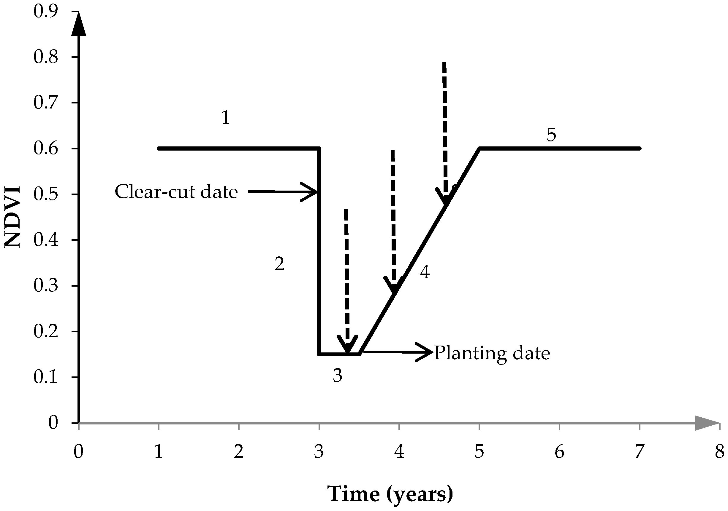
2.1. Eucalyptus Plantations
2.2. Study Area and Construction of the NDVI Time Series


| Sensor Type | Acquisition Date (Year/Day) | Sensor Type | Acquisition Date | ||
|---|---|---|---|---|---|
| 1 | ETM 7+ | 2000/258 | 9 | TM 5 | 2008/320 |
| 2 | TM 5 | 2001/251 | 10 | TM 5 | 2009/290 |
| 3 | ETM 7+ | 2002/311 | 11 | HJ-1A CCD1 | 2010/278 |
| 4 | TM 5 | 2003/338 | 12 | HJ-1B CCD2 | 2011/296 |
| 5 | TM 5 | 2004/325 | 13 | HJ-1B CCD2 | 2012/274 |
| 6 | TM 5 | 2005/346 | 14 | HJ-1A CCD2 | 2013/287 |
| 7 | TM 5 | 2006/266 | 15 | HJ-1A CCD2 | 2014/285 |
| 8 | ETM 7+ | 2007/293 |
| Sensor Type | Path/Row | Band Setting (μm) | Spatial Resolution | Map Projection |
|---|---|---|---|---|
| ETM 7+/TM 5 | 122/43 | 0.45~0.52, 0.52~0.60, 0.63~0.69, 0.76~0.90, 1.55~1.75, 10.4~12.5, 2.08~2.35, (0.5~0.9, ETM 7+ only) | 30 m | UTM 49N, Datum WGS84 |
| HJ-1A/B CCD1/CCD2 | 895/164 | 0.43~0.52, 0.52~0.60, 0.63~0.69, 0.76~0.90 | 30 m | UTM 50N, Datum WGS84 |
2.3. Eucalyptus Classification Methodology
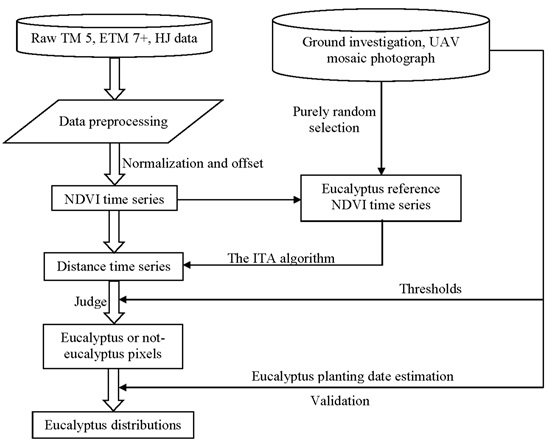
2.3.1. Eucalyptus Classification Steps
2.3.2. Building a Reference NDVI Time Series Sub-Sequence


2.3.3. Eucalyptus Classification Algorithm


2.3.4. Estimation of the Presence and Planting Date of Eucalyptus Plantations
2.4. Comparison with Three Other Classification Algorithms Using a High-Resolution Photograph
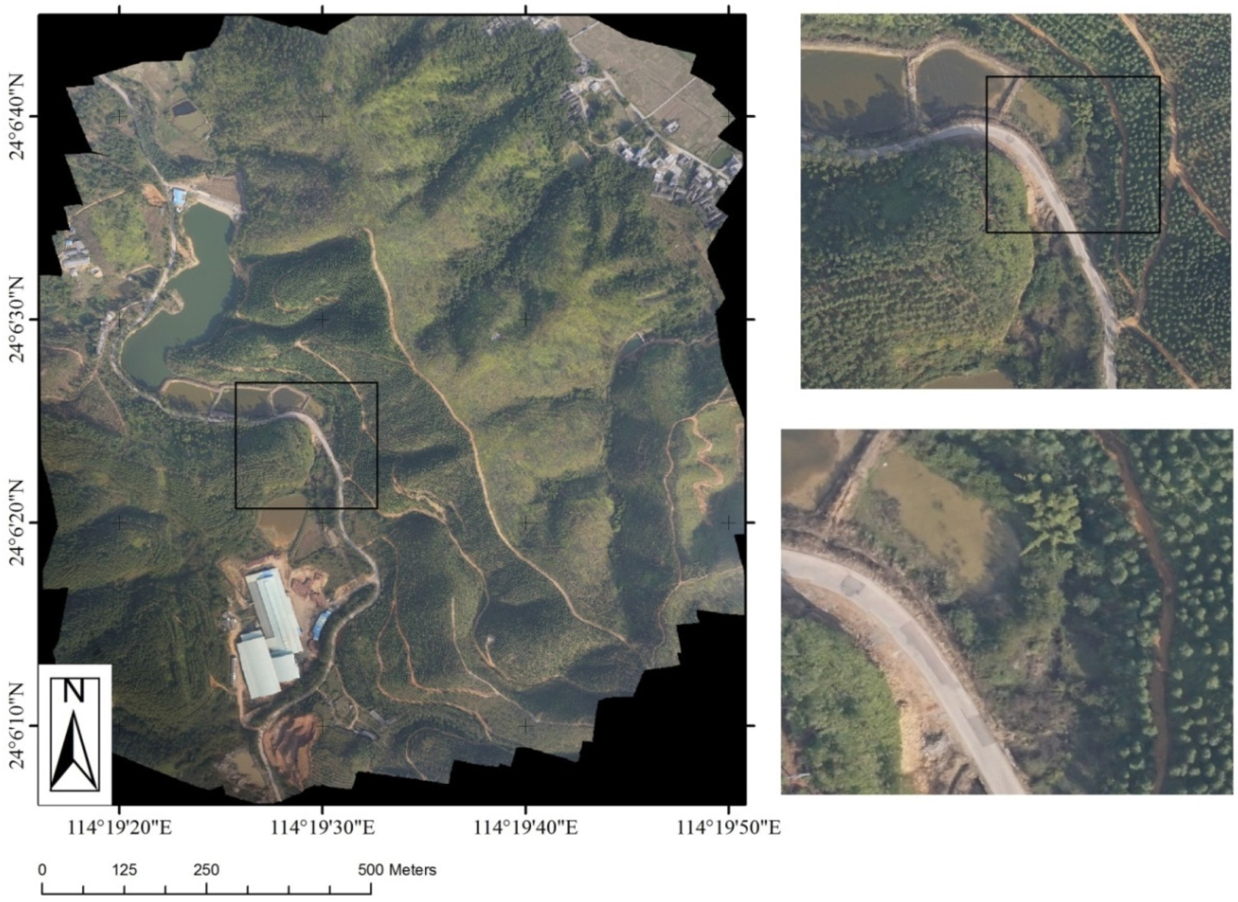
2.4.1. Acquisition of the Validation Photograph
2.4.2. Comparison of Four Discriminant Functions
| Discriminant Functions | Formulas |
|---|---|
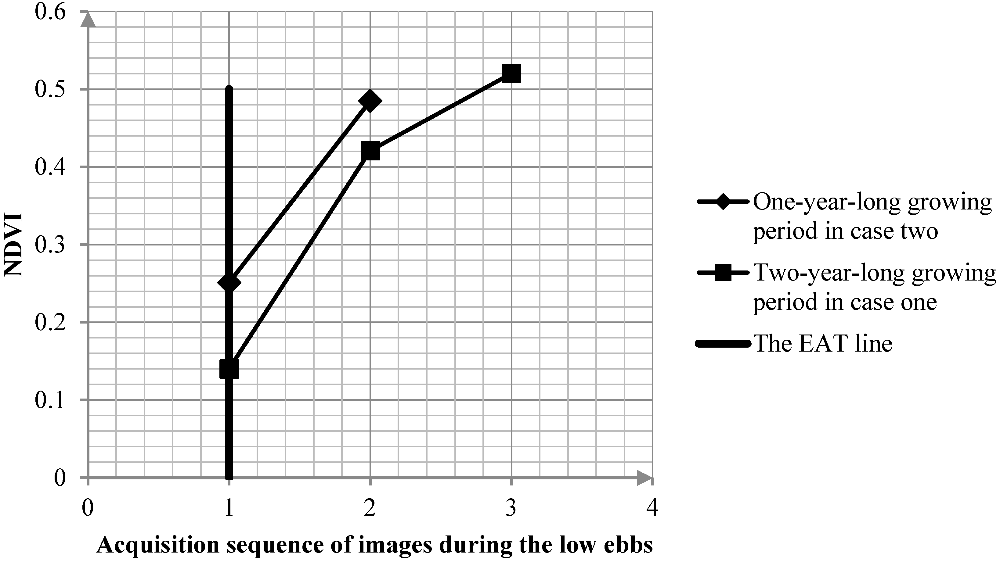
| ITA: Inverted Triangle Area | ; ; , and are the respective ITAs for case one and two. |
| CTB: City Block | was NDVI average value of the ith time step of reference NDVI time series (the same below). |
| SED: Standardized Euclidian Distance | |
| BE: Bounding Envelope | ; , if ; , if ; , elseif |
2.5. Validation of Eucalyptus Classification Results
3. Results and Discussion
3.1. Comparison of the Four Different Classification Algorithms
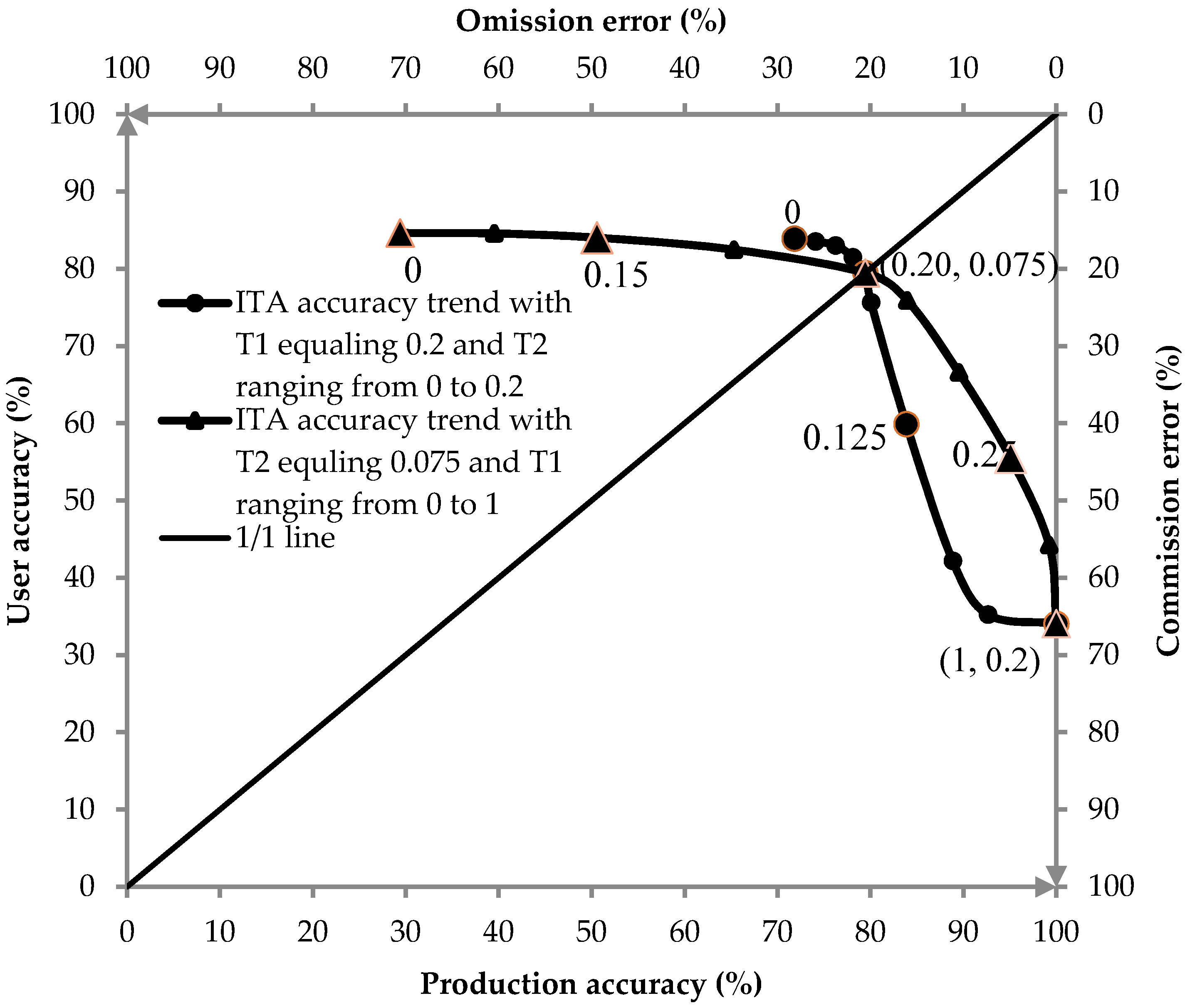
3.1.1. Determination of two Threshold Coefficients

3.1.2. Comparison of Our Results with the Other Classification Algorithms
| Truth Class (from the Mosaic Photograph) | User Accuracy | |||
|---|---|---|---|---|
| Eucalyptus Pixels (Case 1/Case 2) | Not-Eucalyptus Pixels (Case 1/Case 2) | |||
| ITA discriminant function | Eucalyptus pixels | 126/106 | 35/25 | 79% |
| Not-eucalyptus pixels | 60 | 926 | 94% | |
| Producer accuracy | 79% | 94% | Overall acc. 91% | |
| BE discriminant function | Eucalyptus pixels | 169 | 123 | 58% |
| Not-eucalyptus pixels | 123 | 863 | 88% | |
| Producer accuracy | 58% | 88% | Overall acc. 81% | |
| SED discriminant function | Eucalyptus pixels | 145 | 147 | 50% |
| Not-eucalyptus pixels | 147 | 839 | 85% | |
| Producer accuracy | 50% | 85% | Overall acc. 77% | |
| CTB discriminant function | Eucalyptus pixels | 143 | 149 | 49% |
| Not-eucalyptus pixels | 149 | 837 | 85% | |
| Producer accuracy | 49% | 85% | Overall acc. 77% | |
3.2. Further Validation of the Classification Results Using a High-Resolution GF Image

| Truth Class (Interpreted from GF-1 Image) | User Accuracy | |||
|---|---|---|---|---|
| Eucalyptus Pixels | Not-Eucalyptus Pixels | |||
| Classification result of sub-region A | Eucalyptus pixels | 62636 | 20198 | 75.62% |
| Not-eucalyptus pixels | 19141 | 182114 | 90.49% | |
| Producer accuracy | 76.59% | 90.02% | Overall acc 86.15% | |
| Classification result of sub-region B | Eucalyptus pixels | 51319 | 14756 | 77.67% |
| Not-eucalyptus pixels | 15623 | 202391 | 92.83% | |
| Producer accuracy | 76.66% | 93.20% | Overall acc.89.31% | |
3.3. Estimation of the Eucalyptus Planting Date

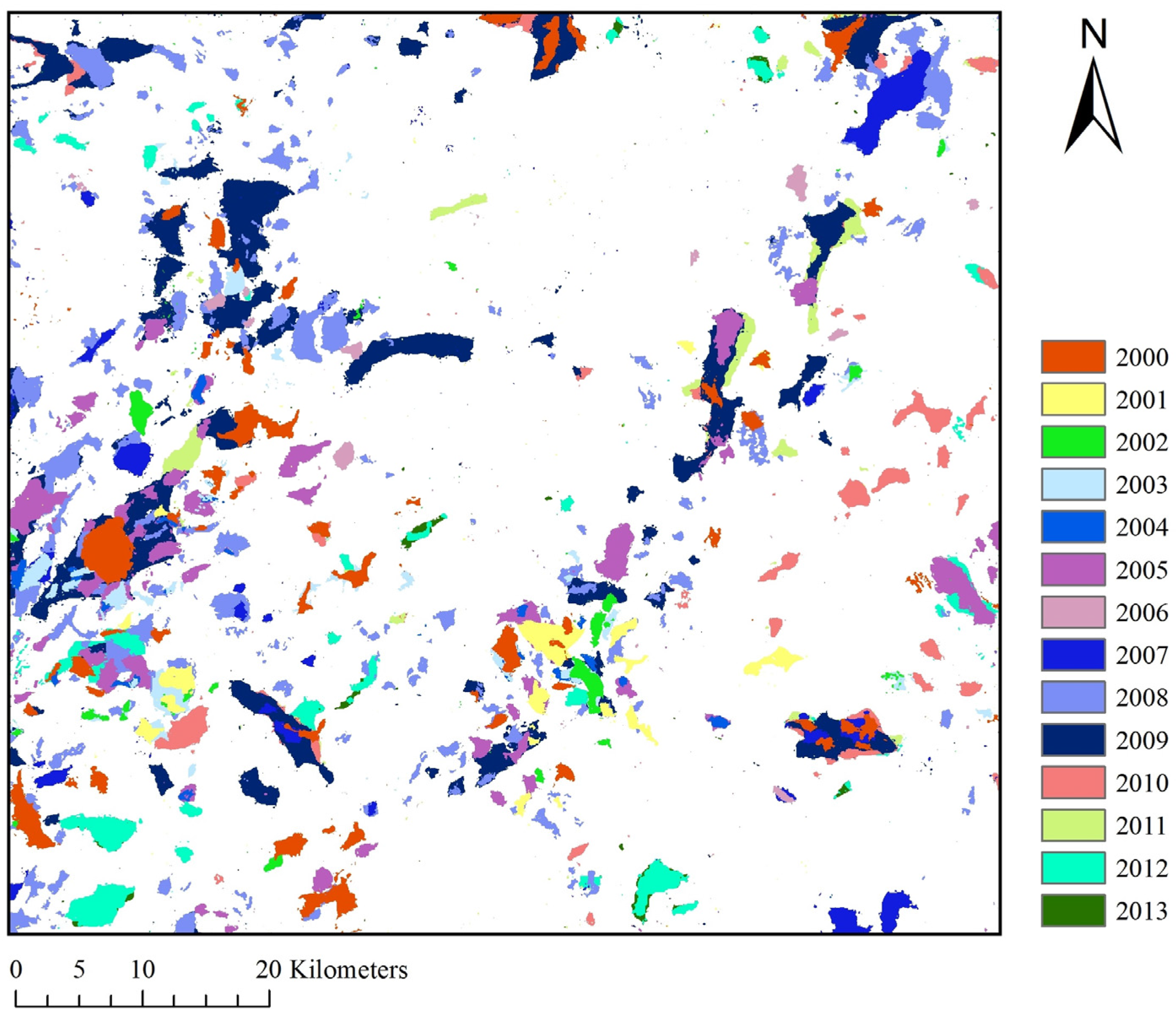
3.4. Eucalyptus Plantation Map Classified with the ITA Algorithm

3.5. Assessment of Eucalyptus Classification
- (1)
- Errors due to different data sources. When building the NDVI time series, we used NDVI from ETM 7+/TM 5 from 2000 to 2009 and NDVI from HJ-1A/B from 2010 to 2014. Although the difference of NDVI from these three sensors was so small (as discussed in Section 2.2) that a process of normalizing NDVI was left out, the classification accuracy of 2008, 2009, 2010 and 2011 (the biggest length of the reference NDVI time series sub-sequence was three time steps) was likely somewhat lower due to the lack of normalization between sensors. For validation, we used the UAV photographs and the GF-1 image. Although all images were pre-processed, many errors, especially those caused by different flight angles and attitudes of satellites could not be avoided [36,37].
- (2)
- Errors due to mixed pixels. In the application of remote sensing data, one pixel necessarily includes information from many different features in addition to the one of interest [6,38]. For example, on the borders of eucalyptus plantations, a eucalyptus pixel may be classified as a not-eucalyptus pixel because of interference from extraneous features (water, bamboo, etc.), thereby decreasing accuracy in these areas. As shown in Figure 8, within the eucalyptus class, numerous vacant regions existed, where the coverage of eucalyptus plantations was low and even some bare soil was exposed, resulting in mixed pixels. Therefore, although the spatial resolution was high in this study, errors from the effect of mixed pixels could not be avoided.
- (3)
- Errors caused by the determination of the reference NDVI time series sub-sequence and threshold coefficients. The reference NDVI time series sub-sequence and threshold coefficients are the basis of the classification algorithms. When determining these coefficients, we considered as many significant factors as we could to build a representative reference time series. However, artificial and systemic factors still existed. We selected a mosaic photograph region to determine threshold coefficients and worked to balance commission and omission errors. Nevertheless, as further validation showed, there remained a small difference between these errors. Our study area was relatively small, so the same threshold coefficients could be shared. Larger study areas will require additional investigations and the adjustment of threshold coefficients for different sub-regions.
3.6. Potential of the ITA Methodology
3.6.1. Potential Improvement of the ITA Methodology
3.6.2. Application Potential of the ITA Methodology
4. Conclusions
Acknowledgments
Author Contributions
Conflicts of Interest
References
- Belward, A.S.; Estes, J.E.; Kline, K.D. The igbp-dis global 1-km land-cover data set discover: A project overview. Photogram. Eng. Remote Sens. 1999, 65, 1013–1020. [Google Scholar]
- Watts, A.C.; Ambrosia, V.G.; Hinkley, E.A. Unmanned aircraft systems in remote sensing and scientific research: Classification and considerations of use. Remote Sens. 2012, 4, 1671–1692. [Google Scholar] [CrossRef]
- Immitzer, M.; Atzberger, C.; Koukal, T. Tree species classification with random forest using very high spatial resolution 8-band worldview-2 satellite data. Remote Sens. 2012, 4, 2661–2693. [Google Scholar] [CrossRef]
- Li, C.C.; Wang, J.; Wang, L.; Hu, L.Y.; Gong, P. Comparison of classification algorithms and training sample sizes in urban land classification with landsat thematic mapper imagery. Remote Sens. 2014, 6, 964–983. [Google Scholar] [CrossRef]
- Kindu, M.; Schneider, T.; Teketay, D.; Knoke, T. Land use/land cover change analysis using object-based classification approach in munessa-shashemene landscape of the ethiopian highlands. Remote Sens. 2013, 5, 2411–2435. [Google Scholar] [CrossRef]
- Desclee, B.; Bogaert, P.; Defourny, P. Forest change detection by statistical object-based method. Remote Sens. Environ. 2006, 102, 1–11. [Google Scholar] [CrossRef]
- Goodenough, D.G.; Dyk, A.; Niemann, O.; Pearlman, J.S.; Chen, H.; Han, T.; Murdoch, M.; West, C. Processing hyperion and ali for forest classification. IEEE Trans. Geosci. Remote Sens. 2003, 41, 1321–1331. [Google Scholar] [CrossRef]
- Xie, Y.C.; Sha, Z.Y.; Yu, M. Remote sensing imagery in vegetation mapping: A review. J. Plant Ecol. 2008, 1, 9–23. [Google Scholar] [CrossRef]
- Vo, Q.T.; Oppelt, N.; Leinenkugel, P.; Kuenzer, C. Remote sensing in mapping mangrove ecosystems—An object-based approach. Remote Sens. 2013, 5, 183–201. [Google Scholar] [CrossRef]
- Christina, M.; Laclau, J.P.; Goncalves, J.L.M.; Jourdan, C.; Nouvellon, Y.; Bouillet, J.P. Almost symmetrical vertical growth rates above and below ground in one of the world’s most productive forests. Ecosphere 2011, 2. [Google Scholar] [CrossRef]
- Turner, J.; Lambert, M. Change in organic carbon in forest plantation soils in eastern australia. For. Ecol. Manag. 2000, 133, 231–247. [Google Scholar] [CrossRef]
- Gardner, T.A.; Hernandez, M.I.M.; Barlow, J.; Peres, C.A. Understanding the biodiversity consequences of habitat change: The value of secondary and plantation forests for neotropical dung beetles. J. Appl. Ecol. 2008, 45, 883–893. [Google Scholar] [CrossRef]
- Xu, M.; Watanachaturaporn, P.; Varshney, P.K.; Arora, M.K. Decision tree regression for soft classification of remote sensing data. Remote Sens. Environ. 2005, 97, 322–336. [Google Scholar] [CrossRef]
- Bannari, A.; Chevrier, M.; Staenz, K.; McNairn, H. Senescent vegetation and crop residue mapping in agricultural lands using artificial neutral networks and hyperspectral remote sensing. In Proceedings of the 2003 IEEE International Geoscience and Remote Sensing Symposium, Ontario, ON, Canada, 21–25 July 2003.
- Kayitakire, F.; Hamel, C.; Defourny, P. Retrieving forest structure variables based on image texture analysis and ikonos-2 imagery. Remote Sens. Environ. 2006, 102, 390–401. [Google Scholar] [CrossRef]
- Yu, Q.; Gong, P.; Clinton, N.; Biging, G.; Kelly, M.; Schirokauer, D. Object-based detailed vegetation classification. With airborne high spatial resolution remote sensing imagery. Photogram. Eng. Remote Sens. 2006, 72, 799–811. [Google Scholar] [CrossRef]
- Lu, H.; Raupach, M.R.; McVicar, T.R.; Barrett, D.J. Decomposition of vegetation cover into woody and herbaceous components using avhrr ndvi time series. Remote Sens. Environ. 2003, 86, 1–18. [Google Scholar] [CrossRef]
- Wardlow, B.D.; Egbert, S.L. Large-area crop mapping using time-series modis 250 m ndvi data: An assessment for the us central great plains. Remote Sens. Environ. 2008, 112, 1096–1116. [Google Scholar] [CrossRef]
- Pan, Y.Z.; Li, L.; Zhang, J.S.; Liang, S.L.; Zhu, X.F.; Sulla-Menashe, D. Winter wheat area estimation from modis-evi time series data using the crop proportion phenology index. Remote Sens. Environ. 2012, 119, 232–242. [Google Scholar] [CrossRef]
- Muhammad, S.; Niu, Z.; Wang, L.; Aablikim, A.; Hao, P.Y.; Wang, C.Y. Crop classification based on time series modis evi and ground observation for three adjoining years in xinjiang. Spectrosc. Spectr. Anal. 2015, 35, 1345–1350. [Google Scholar]
- Le Maire, G.; Dupuy, S.; Nouvellon, Y.; Loos, R.A.; Hakarnada, R. Mapping short-rotation plantations at regional scale using modis time series: Case of eucalypt plantations in brazil. Remote Sens. Environ. 2014, 152, 136–149. [Google Scholar] [CrossRef]
- Gao, F.; Masek, J.; Schwaller, M.; Hall, F. On the blending of the landsat and modis surface reflectance: Predicting daily landsat surface reflectance. IEEE Trans. Geosci. Remote Sens. 2006, 44, 2207–2218. [Google Scholar]
- Sellers, P.J. Canopy reflectance, photosynthesis, and transpiration, II. The role of biophysics in the linearity of their interdependence. Remote Sens. Environ. 1987, 21, 143–183. [Google Scholar] [CrossRef]
- Sellers, P.J. Canopy reflectance, photosynthesis and transpiration. Int. J. Remote Sens. 1985, 6, 1335–1372. [Google Scholar] [CrossRef]
- Gausman, H.W. Leaf reflectance of near-infrared. Photogram. Eng. 1974, 40, 183–191. [Google Scholar]
- Paruelo, J.M.; Epstein, H.E.; Lauenroth, W.K.; Burke, I.C. Anpp estimates from ndvi for the central grassland region of the united states. Ecology 1997, 78, 953–958. [Google Scholar] [CrossRef]
- Decker, W.L.; Hayes, M.J. Using noaa avhrr data to estimate maize production in the united states corn belt. Int. J. Remote Sens. 1996, 17, 3189–3200. [Google Scholar]
- le Maire, G.; Marsden, C.; Verhoef, W.; Ponzoni, F.J.; Lo Seen, D.; Begue, A.; Stape, J.L.; Nouvellon, Y. Leaf area index estimation with modis reflectance time series and model inversion during full rotations of eucalyptus plantations. Remote Sens. Environ. 2011, 115, 586–599. [Google Scholar] [CrossRef]
- Chen, J.; Zhu, X.; Vogelmann, J.E.; Gao, F.; Jin, S. A simple and effective method for filling gaps in landsat etm plus slc-off images. Remote Sens. Environ. 2011, 115, 1053–1064. [Google Scholar] [CrossRef]
- Zhu, X.L.; Liu, D.S.; Chen, J. A new geostatistical approach for filling gaps in landsat etm plus slc-off images. Remote Sens. Environ. 2012, 124, 49–60. [Google Scholar] [CrossRef]
- Teillet, P.M.; Staenz, K.; Williams, D.J. Effects of spectral, spatial, and radiometric characteristics on remote sensing vegetation indices of forested regions. Remote Sens. Environ. 1997, 61, 139–149. [Google Scholar] [CrossRef]
- Hao, P.; Wang, L.; Niu, Z.; Aablikim, A.; Huang, N.; Xu, S.; Chen, F. The potential of time series merged from Landsat-5 tm and HJ-1 CCD for crop classification: A case study for bole and manas counties in xinjiang, china. Remote Sens. 2014, 6, 7610–7631. [Google Scholar] [CrossRef]
- le Maire, G.; Marsden, C.; Nouvellon, Y.; Grinand, C.; Hakamada, R.; Stape, J.-L.; Laclau, J.-P. MODIS NDVI time-series allow the monitoring of eucalyptus plantation biomass. Remote Sens. Environ. 2011, 115, 2613–2625. [Google Scholar] [CrossRef]
- The China Centre for Resource Satellite Data and Applications. Available online: http://www.cresda.com/site1/Satellite/3076.shtml (accessed on 9 September 2015).
- Boschetti, L.; Flasse, S.P.; Brivio, P.A. Analysis of the conflict between omission and commission in low spatial resolution dichotomic thematic products: The pareto boundary. Remote Sens. Environ. 2004, 91, 280–292. [Google Scholar] [CrossRef]
- Congalton, R.G. A review of assessing the accuracy of classifications of remotely sensed data. Remote Sens. Environ. 1991, 37, 35–46. [Google Scholar] [CrossRef]
- Congalton, R.G. Putting the Map Accuracy Map Back in Assessment; CRC Press: Boca Raton, FL, America, 2004; pp. 1–11. [Google Scholar]
- Tao, X.T.; Wang, B.; Zhang, L.M. Orthogonal bases approach for the decomposition of mixed pixels in hyperspectral imagery. IEEE Geosci. Remote Sens. Lett. 2009, 6, 219–223. [Google Scholar]
© 2016 by the authors; licensee MDPI, Basel, Switzerland. This article is an open access article distributed under the terms and conditions of the Creative Commons by Attribution (CC-BY) license (http://creativecommons.org/licenses/by/4.0/).
Share and Cite
Qiao, H.; Wu, M.; Shakir, M.; Wang, L.; Kang, J.; Niu, Z. Classification of Small-Scale Eucalyptus Plantations Based on NDVI Time Series Obtained from Multiple High-Resolution Datasets. Remote Sens. 2016, 8, 117. https://doi.org/10.3390/rs8020117
Qiao H, Wu M, Shakir M, Wang L, Kang J, Niu Z. Classification of Small-Scale Eucalyptus Plantations Based on NDVI Time Series Obtained from Multiple High-Resolution Datasets. Remote Sensing. 2016; 8(2):117. https://doi.org/10.3390/rs8020117
Chicago/Turabian StyleQiao, Hailang, Mingquan Wu, Muhammad Shakir, Li Wang, Jun Kang, and Zheng Niu. 2016. "Classification of Small-Scale Eucalyptus Plantations Based on NDVI Time Series Obtained from Multiple High-Resolution Datasets" Remote Sensing 8, no. 2: 117. https://doi.org/10.3390/rs8020117