
Regional Mapping of Plantation Extent Using Multisensor Imagery

Abstract
:
1. Introduction
2. Materials and Methods
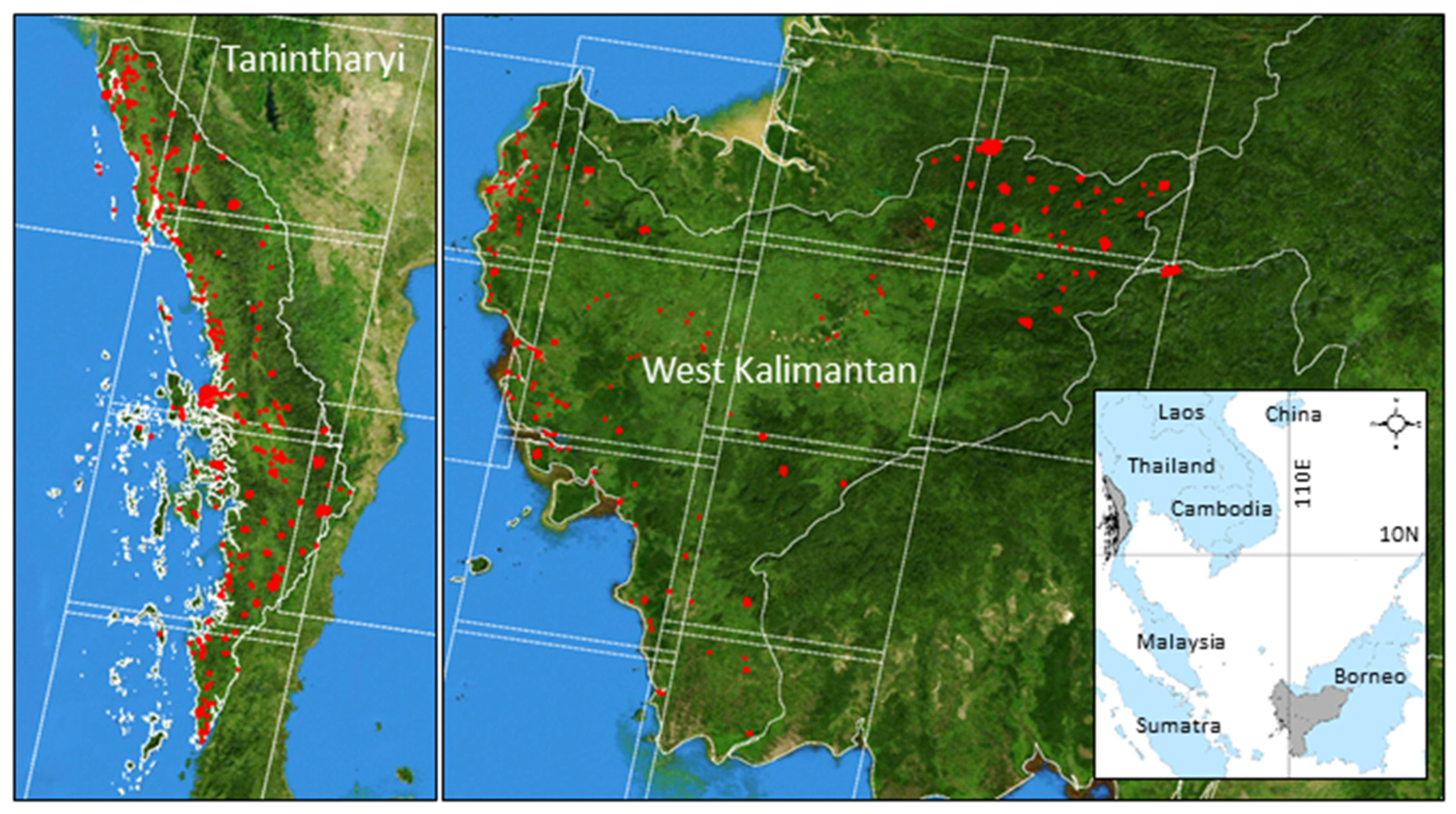
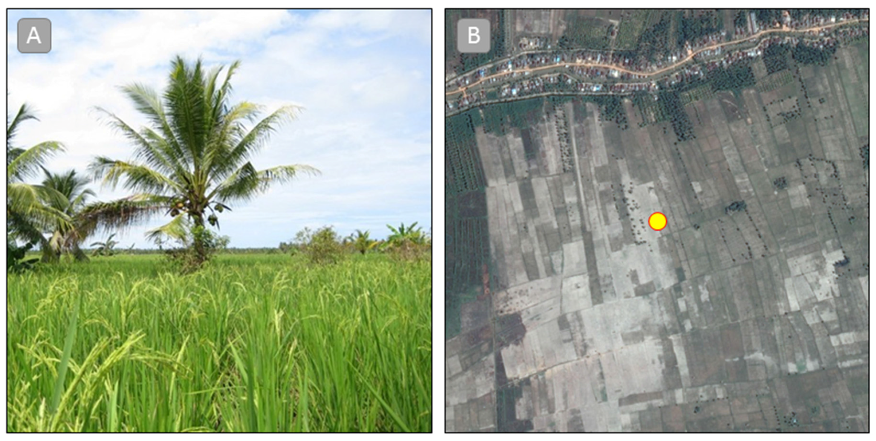
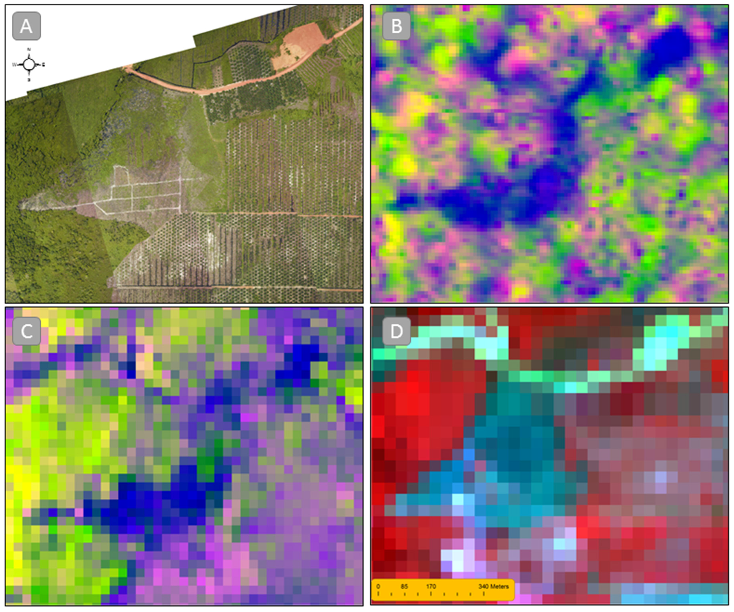
2.1. Study Areas
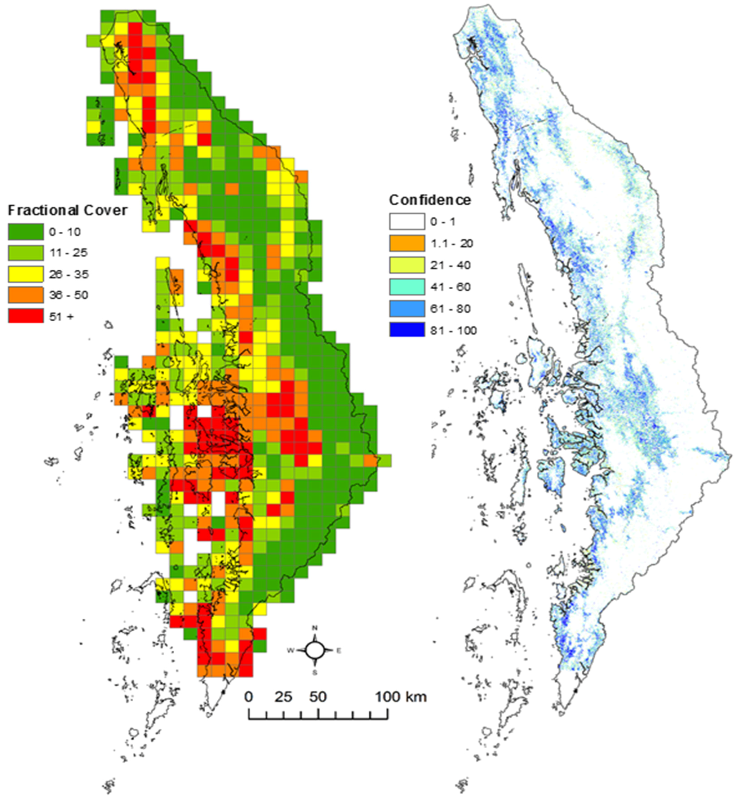
2.1.1. Tanintharyi, Myanmar
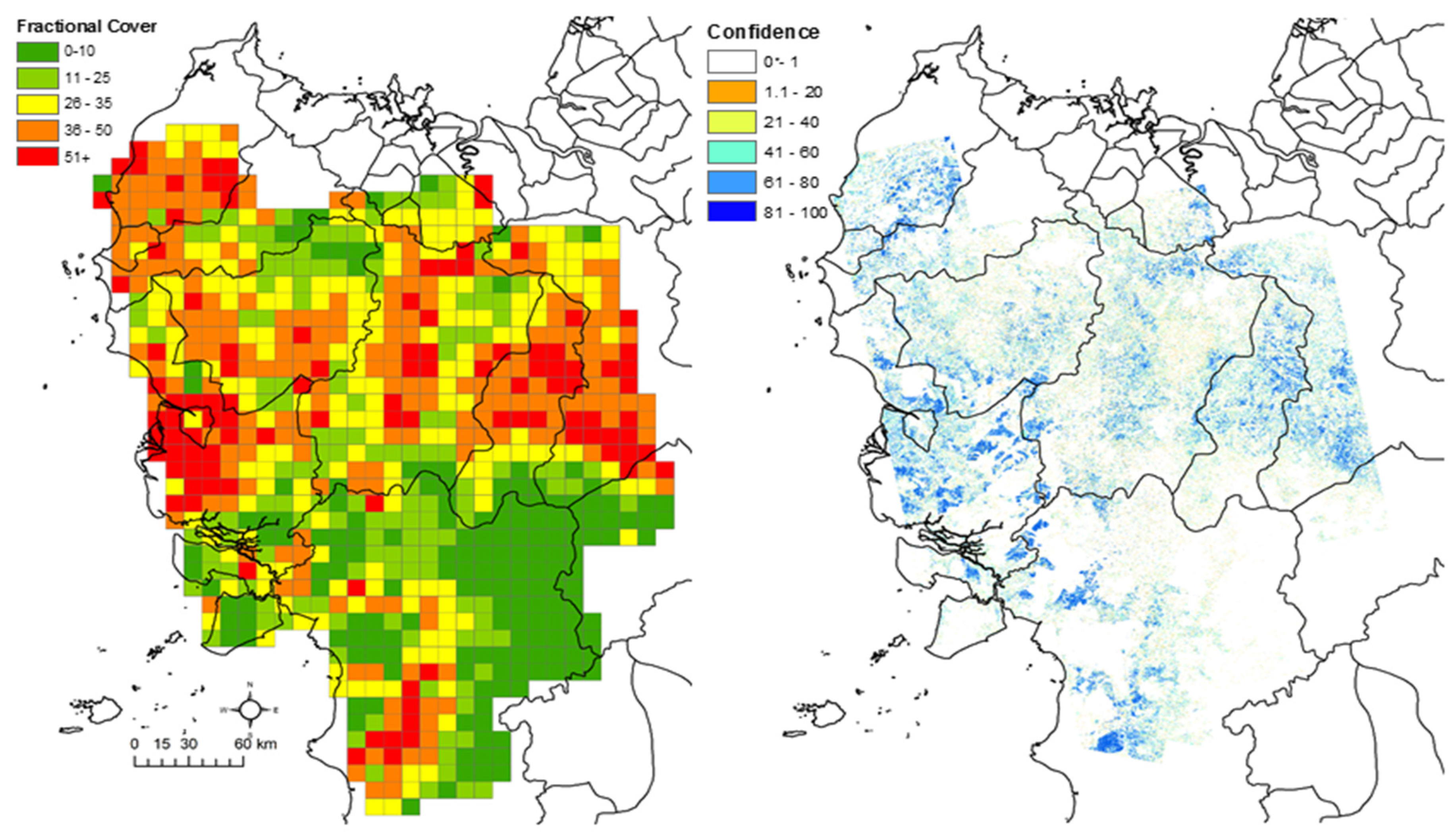
2.1.2. West Kalimantan
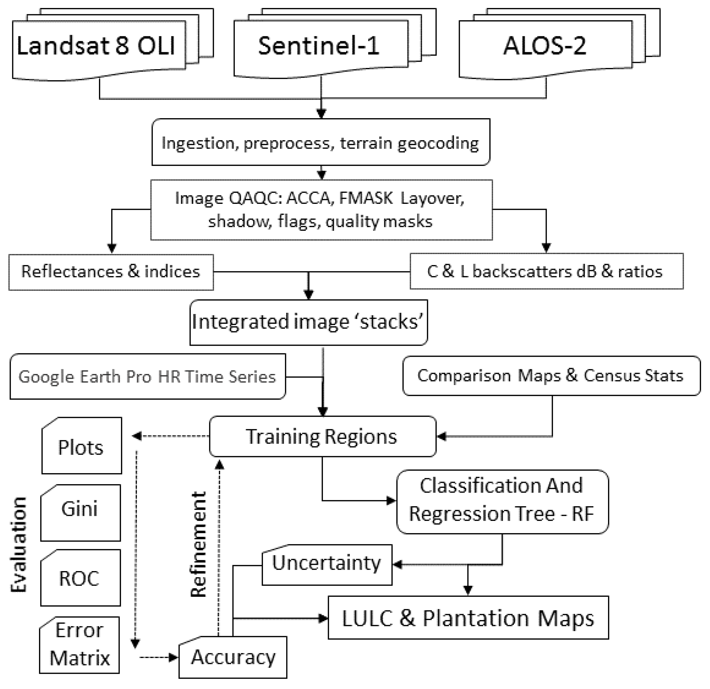
2.2. Data Preprocessing
2.2.1. ALOS-2 PALSAR-2
2.2.2. Sentinel-1A
2.2.3. Landsat-OLI
2.3. Mapping Approach
3. Results and Discussion
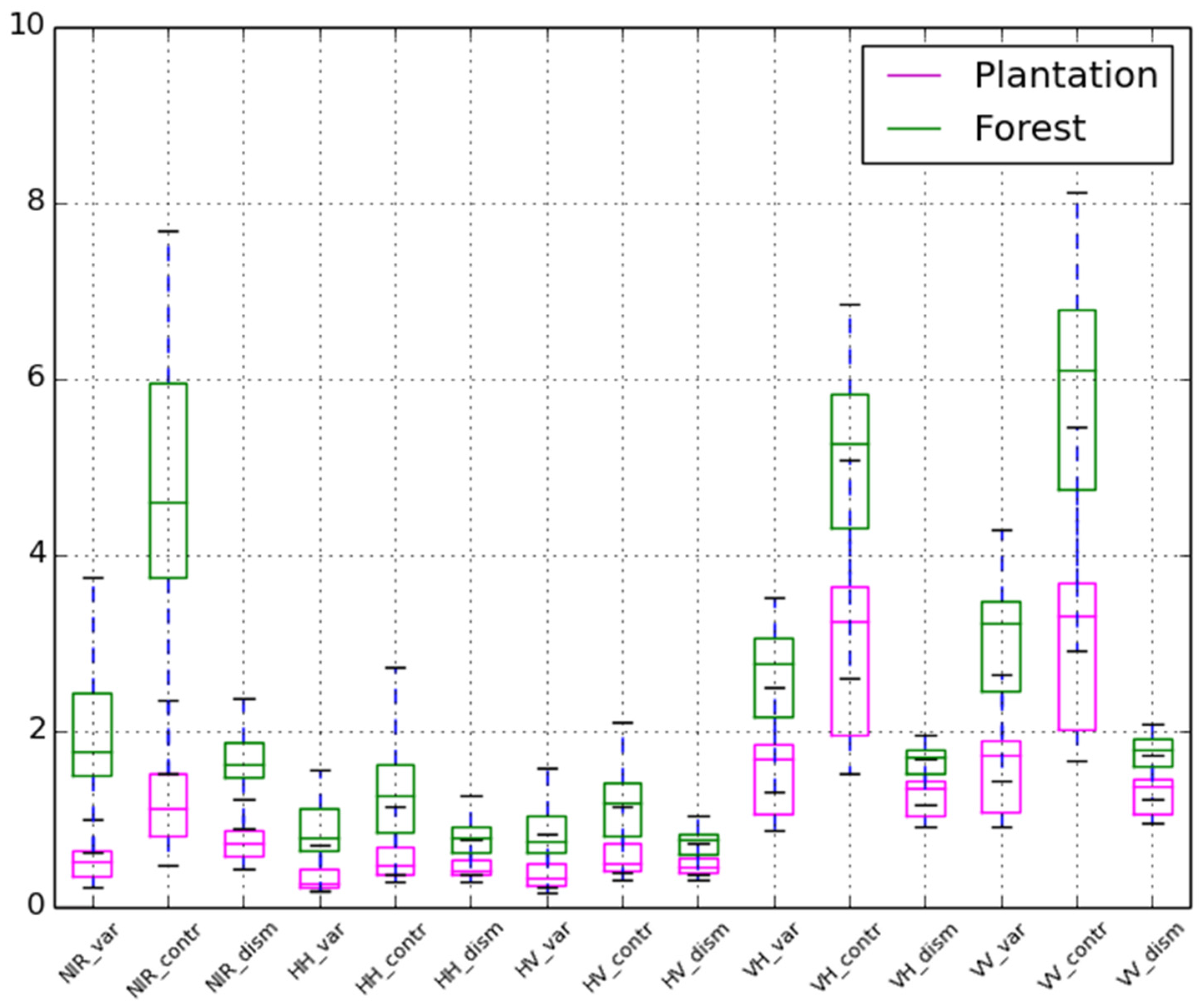
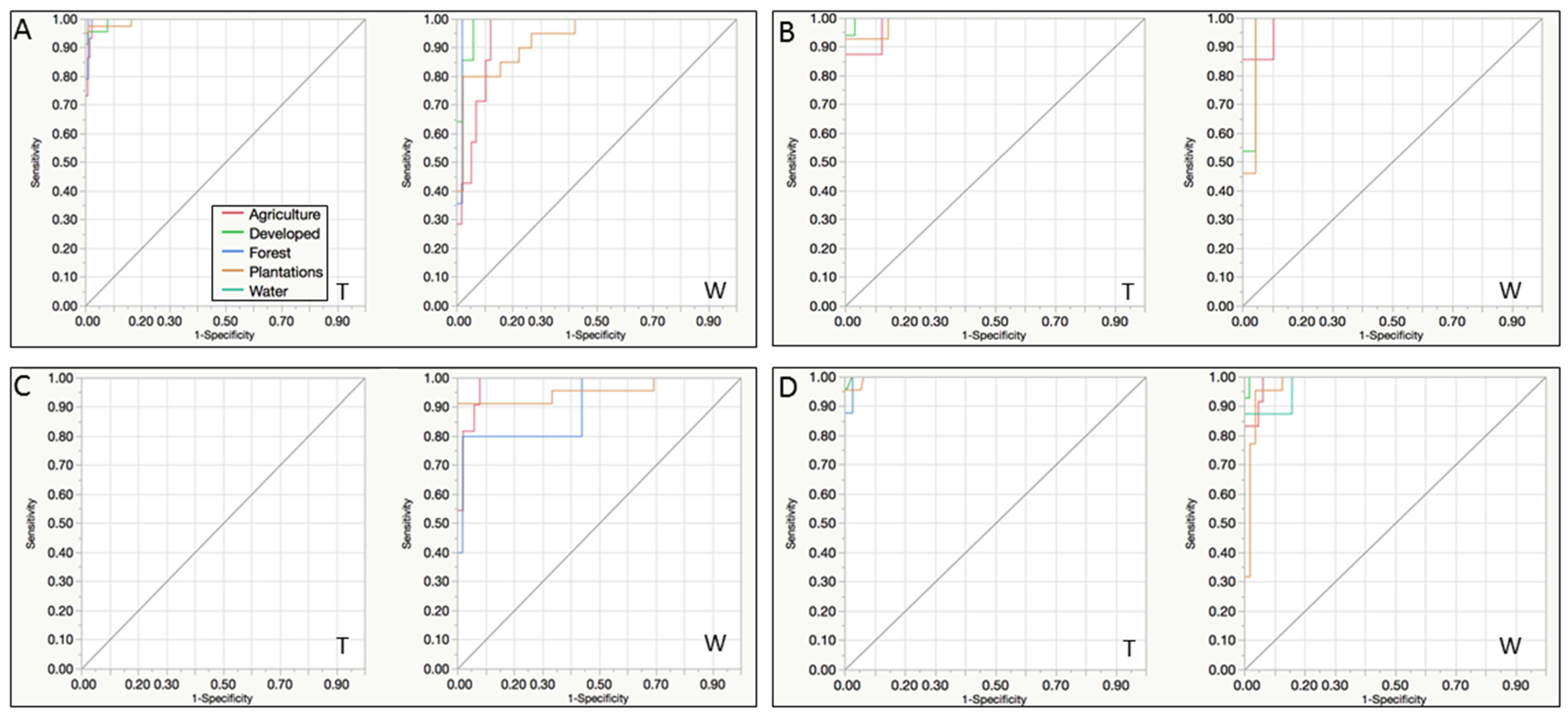
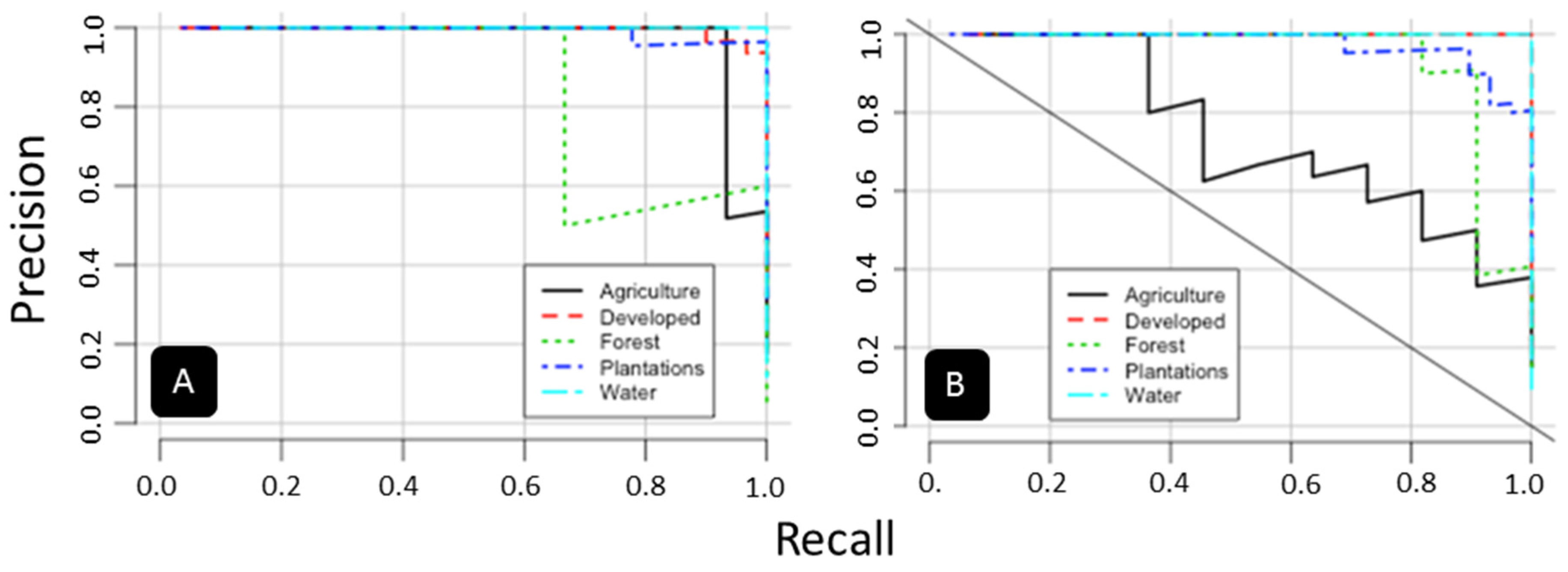
3.1. Data Mining
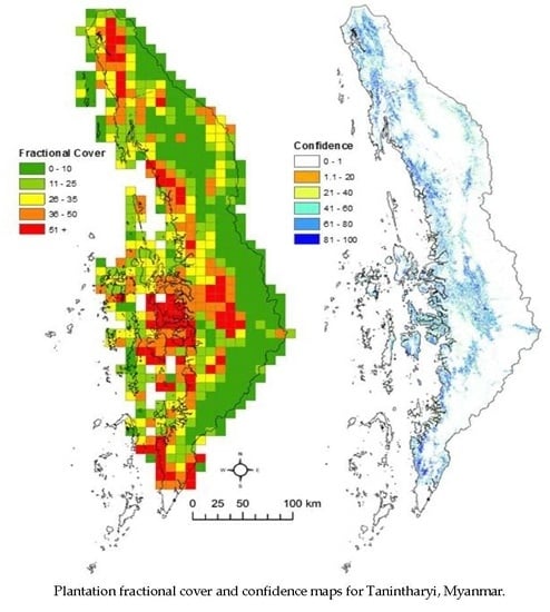
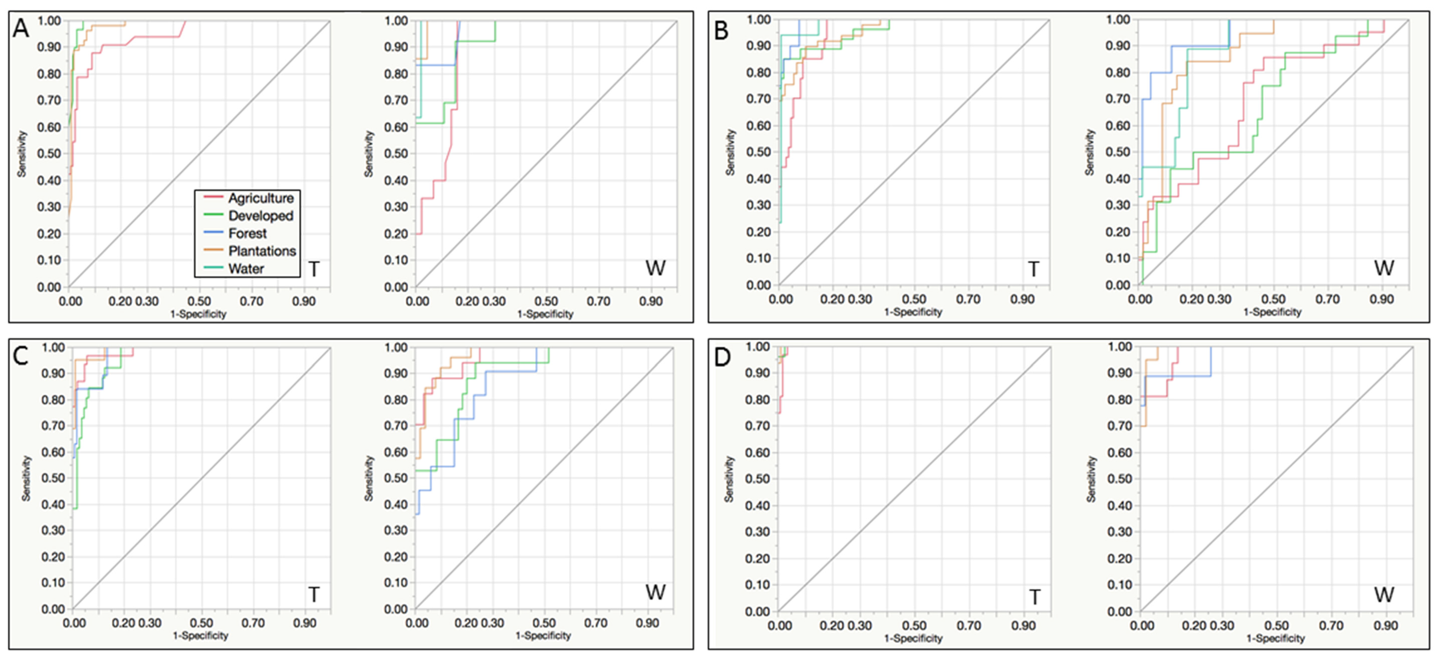
3.2. Mapping
4. Conclusions
Supplementary Files
Supplementary File 1Acknowledgments
Author Contributions
Conflicts of Interest
References
- Food and Agriculture Organization of the United Nations. FRA 2000 Main Report; FAO: Rome, Italy, 2001. [Google Scholar]
- Food and Agriculture Organization of the United Nations. Global Forest Resources Assessment 2005, Main Report; FAO: Rome, Italy, 2006. [Google Scholar]
- Miettinen, J.; Hooijer, A.; Shi, C.; Tollenaar, D.; Vernimmen, R.; Liew, S.C.; Malins, C.; Page, S.E. Extent of industrial plantations on Southeast Asian peatlands in 2010 with analysis of historical expansion and future projections. Glob. Chang. Biol. Bioenergy 2012, 4, 908–918. [Google Scholar] [CrossRef]
- Li, Z.; Fox, J.M. Mapping rubber tree growth in mainland Southeast Asia using time-series MODIS 250 m NDVI and statistical data. Appl. Geogr. 2012, 32, 420–432. [Google Scholar] [CrossRef]
- Zhai, D.L.; Cannon, C.H.; Slik, J.W.F.; Zhang, C.P.; Dai, Z.C. Rubber and pulp plantations represent a double threat to Hainan’s natural tropical forests. J. Environ. Manag. 2012, 96, 64–73. [Google Scholar] [CrossRef] [PubMed]
- Broich, M.; Hansen, M.C.; Potapov, P.; Adusei, B.; Lindquist, R.; Stehman, S.V. Time-series analysis of multi-resolution optical imagery for quantifying forest cover loss in Sumatra and Kalimantan, Indonesia. Int. J. Appl. Earth Obs. Geoinf. 2011, 13, 277–291. [Google Scholar] [CrossRef]
- Carlson, K.M.; Curran, L.M.; Asner, G.P.; Pittman, A.M.; Trigg, S.N.; Adeney, J.M. Carbon emissions from forest conversion by Kalimantan oil palm plantations. Nat. Clim. Chang. 2013, 3, 283–287. [Google Scholar] [CrossRef]
- Somers, B.; Verbesselt, J.; Ampe, E.M.; Sims, N.; Verstraeten, W.W.; Coppin, P. Spectral mixture analysis to monitor defoliation in mixed-aged Eucalyptus globulus Labill plantations in southern Australia using Landsat 5-TM and EO-1 Hyperion data. Int. J. Appl. Earth Obs. Geoinf. 2010, 12, 270–277. [Google Scholar] [CrossRef]
- Le Maire, G.; Marsden, C.; Nouvellon, Y.; Grinand, C.; Hakamda, R.; Stape, J.L.; Laclau, J.P. MODIS NDVI time-series allow the monitoring of Eucalyptus plantation biomass. Remote Sens. Environ. 2011, 115, 2613–2625. [Google Scholar] [CrossRef]
- Win, R.N.; Reiji, S.; Shinya, T. Forest cover changes under selective logging in the Kabaung Reserved Forest, Bago Mountains, Myanmar. Mt. Res. Dev. 2009, 29, 328–338. [Google Scholar] [CrossRef]
- Larsson, H. Linear regressions for canopy cover estimation in Acacia woodlands using Landsat-TM, Landsat-MSS, ans SPOT HRV XS data. Int. J. Remote Sens. 1993, 14, 2129–2136. [Google Scholar] [CrossRef]
- De Asis, A.M.; Omasa, K.; Oki, K.; Shimizu, Y. Accuracy and applicability of linear spectral unmixing in delineating potential erosion areas in tropical watersheds. Int. J. Remote Sens. 2008, 29, 4151–4171. [Google Scholar] [CrossRef]
- Vina, A.; Bearer, S.; Zhang, H.; Ouyang, Z.; Liu, J. Evaluating MODIS data for mapping wildlife habitat distribution. Remote Sens. Environ. 2008, 112, 2160–2169. [Google Scholar] [CrossRef]
- Xu, X.; Zhou, G.; Du, H.; Partida, A. Bamboo forest change and its effect on biomass carbon stocks: A case study of Anji County, Zhejiang Province, China. J. Trop. For. Sci. 2012, 24, 426–435. [Google Scholar]
- Rosenqvist, A. Evaluation of JERS-1, ERS-1 and Almaz SAR backscatter for rubber and oil palm stands in West Malaysia. Int. J. Remote Sens. 1996, 17, 3219–3231. [Google Scholar] [CrossRef]
- Koh, L.P.; Miettinen, J.; Liew, S.C.; Ghazoul, J. Remotely sensed evidence of tropical peatland conversion to oil palm. Proc. Natl. Acad. Sci. USA 2011, 108, 5127–5132. [Google Scholar] [CrossRef] [PubMed]
- Miettinen, J.; Shi, C.; Liew, S.C. Deforestation rates in insular Southeast Asia between 2000 and 2010. Glob. Chang. Biol. 2011, 17. [Google Scholar] [CrossRef]
- Dong, J.; Xiao, X.; Sheldon, S.; Biradar, C.; Xie, G. Mapping topical forests and rubber plantations in complex landscapes by integrating PALSAR and MODIS imagery. ISPRS J. Photogramm. Remote Sens. 2012, 74, 20–33. [Google Scholar] [CrossRef]
- Dong, J.; Xiao, X.; Chen, B.; Torbick, N.; Jin, C.; Zhang, G.; Biradar, C. Mapping deciduous rubber plantation through integration of PALSAR and time-series Landsat imagery. Remote Sens. Environ. 2013, 134, 392–402. [Google Scholar] [CrossRef]
- Gutierrez-Velez, V.H.; DeFries, R. Annual multi-resolution detection of land cover conversion to oil palm in the Peruvian Amazon. Remote Sens. Environ. 2013, 129, 154–167. [Google Scholar] [CrossRef]
- Kou, W.; Xiao, X.; Dong, J.; Gan, J.; Zhai, D.; Zhang, G.; Qin, Y.; Li, L. Mapping deciduous rubber plantation areas and stand ages with PALSAR and Landsat images. Remote Sens. 2015, 71, 1048–1073. [Google Scholar] [CrossRef]
- Woods, K. Commercial Agriculture Expansion in Myanmar: Links to Deforestation, Conversion Timber, and Land Conflicts; Forest Trends Report Series; Forest Trends Association: Washington, DC, USA, 2013; p. 78. [Google Scholar]
- Woods, K.; Kerstin, C. Baseline Study 4, Myanmar: Overview of Forest Law Enforcement Governance and Trade; Forest Trends: Washington, DC, USA, 2011. [Google Scholar]
- Miettinen, J.; Shi, C.; Liew, S. Twodecades of destruction in Southeast Asia’ peat swamp forests. Front. Ecol. Environ. 2011, 10, 124–128. [Google Scholar] [CrossRef]
- Masek, J.G.; Vermote, E.F.; Saleous, N.E.; Wolfe, R.; Hall, F.G.; Huemmrich, K.F.; Gao, F.; Kutler, J.; Lim, T.K. A Landsat surface reflectance dataset for North America, 1990–2000. IEEE Geosci. Remote Sens. Lett. 2006, 3, 68–72. [Google Scholar] [CrossRef]
- Vermote, E.F.; El Saleous, N.; Justice, C.O.; Kaufman, Y.J.; Privette, J.L.; Remer, L.; Roger, J.C.; Tanré, D. Atmospheric correction of visible to middle-infrared EOS-MODIS data over land surfaces: Back-ground, operational algorithm and validation. J. Geophys. Res. Atmos. 1997, 102, 17131–17141. [Google Scholar] [CrossRef]
- Zhu, Z.; Woodcock, C. Object-based cloud and cloud shadow detection in Landsat imagery. Remote Sens. Environ. 2012, 118, 83–94. [Google Scholar] [CrossRef]
- Vermote, E.F.; Kotchenova, S. Atmospheric correction for the monitoring of land surfaces. J. Geophys. Res. 2008, 113. [Google Scholar] [CrossRef]
- Irish, R.; Barker, J.; Goward, S.; Arvidson, T. Characterization of the Landsat 7 ETM+ automated cloud cover assessment (ACCA) algorithm. Photogramm. Eng. Remote Sens. 2006, 72, 1179–1188. [Google Scholar] [CrossRef]
- Rouse, J.; Haas, J.; Schell, J.; Deering, D. Monitoring vegetation systems in the Great Plains with ERTS. In Proceedings of the Third ERTS Symposium, Washington, DC, USA, 10 December 1974; pp. 309–317.
- Tucker, C. Red and photographic infrared linear combinations for monitoring vegetation. Remote Sens. Environ. 1979, 8, 127–150. [Google Scholar] [CrossRef]
- Torbick, N.; Salas, W.; Xiao, X.; Ingraham, P.; Fearon, M.G.; Biradarm, C.; Zhao, D.; Liu, Y.; Li, P.; Zhao, Y. Integrating SAR and optical imagery for regional mapping of paddy rice attributes in the Poyang Lake Watershed, China. Can. J. Remote Sens. 2011, 37, 17–26. [Google Scholar] [CrossRef]
- Xiao, X.; Boles, S.; Liu, J.; Zhuang, D.; Liu, M. Characterization of forest types in Northeastern China, using multi-temporal SPOT-4 VEGETATION sensor data. Remote Sens. Environ. 2002, 82, 335–348. [Google Scholar] [CrossRef]
- Daughtry, C.; Hunt, E.; Doraiswamy, P.; McMurtrey, J. Remote sensing the spatial distribution of crop residues. Agron. J. 2005, 97, 868–871. [Google Scholar] [CrossRef]
- Hagen, S.; Heilman, P.; Marsett, R.; Torbick, N.; Salas, W.; Ravensway, J.; Qi, J. Mapping total vegetation cover across western rangelands with MODIS data. Rangel. Ecol. Manag. 2012, 65, 456–467. [Google Scholar] [CrossRef]
- Earth Observation and Modeling. Available online: www.eomf.ou.edu/photos/ (accessed on 25 January 2016).
- Thapa, R.; Watanabe, M.; Motohka, T.; Shimada, M. Potential of high-resolution ALOS-PALSAR mosaic texture for aboveground forest carbon tracking in tropical region. Remote Sens. Environ. 2015, 160, 122–133. [Google Scholar] [CrossRef]
- Haralick, R.; Shanmugam, K.; Dinstein, I. Textural features for image classification. IEEE Trans. Syst. Man Cybern. 1973, 6, 610–621. [Google Scholar] [CrossRef]
- Breiman, L. Random forests. Mach. Learn. 2001, 45, 5–32. [Google Scholar] [CrossRef]
- Lawrence, R.; Wood, S.; Sheley, R. Mapping invasive plants using hyperspectral imagery and Breiman cutler classifications (RandomForest). Remote Sens. Environ. 2006, 100, 356–362. [Google Scholar] [CrossRef]
- Watts, J.; Lawrence, R.; Miller, P.; Montagne, C. Monitoring of cropland practices for carbon sequestration purposes in north central Montana by Landsat remote sensing. Remote Sens. Environ. 2009, 113, 1843–1852. [Google Scholar] [CrossRef]
- Schultz, B.; Immitzer, M.; Formaggio, A.R.; Sanches, I.D.A.; Luiz, A.J.B.; and Atzberger, C. Self-guided segmentation and classification of multi-temporal Landsat 8 images for crop type mapping in southwestern Brazil. Remote Sens. 2015, 7, 14482–14508. [Google Scholar] [CrossRef]
- Whitcomb, J.; Moghaddam, M.; McDonlad, K.; Kellndorf, J.; Podest, E. Mapping vegetated wetlands of Alaska using L-band radar satellite imagery. Can. J. Remote Sens. 2009, 35, 54–72. [Google Scholar] [CrossRef]
- Torbick, N.; Persson, A.; Olefeldt, D.; Frolking, S.; Salas, W.; Hagen, S.; Crill, P.; Li, C. High resolution mapping of peatland hydroperiod at a high-latitude Swedish mire. Remote Sens. 2012, 4, 1974–1994. [Google Scholar] [CrossRef]
- Torbick, N.; Salas, W. Mapping agricultural wetlands in the Sacramento Valley, USA with satellite remote sensing. Wetlands Ecol. Manag. 2014, 23, 79–94. [Google Scholar] [CrossRef]
- Wilkes, P.; Jones, S.D.; Suarez, L.; Mellor, A.; Woodgate, W.; Soto-Berelov, M.; Haywood, A.; Skidmore, A.K. Mapping forest canopy height over large areas by upscaling ALS estimates with freely available satellite data. Remote Sens. 2015, 7, 12563–12587. [Google Scholar] [CrossRef]
- Song, W.; Dolon, J.M.; Cline, D.; Xiong, G. Leanring-based algal bloom event recognition for oceanographic decision support system using remote sensing data. Remote Sens. 2015, 7, 13564–13585. [Google Scholar] [CrossRef]
- Torbick, N.; Corbiere, M. Mapping urban sprawl and impervious surfaces in the northeast United States for the past four decades. GISci. Remote Sens. 2015, 52, 746–764. [Google Scholar] [CrossRef]
- Karlson, M.; Ostwald, M.; Reese, H.; Sanou, J.; Tankoano, B.; Mattsson, E. Mapping tree canopy cover and aboveground biomass in Sudano-Sahelian woodlands using Landsat 8 and random forest. Remote Sens. 2015, 7, 10017–10041. [Google Scholar] [CrossRef]
- Mitchard, E.T.; Saatchi, S.S.; White, L.J.T.; Abernethy, K.A.; Jeffery, K.J.; Lewis, S.L.; Collins, M.; Lefsky, M.A.; Leal, M.E.; Woodhouse, E.H.; et al. Mapping tropical forest biomass with radar and spaceborne LiDAR in Lop’e National Park, Gabon: Overcoming problems of high biomass and persistent cloud. Biogeosciences 2012, 9, 179–191. [Google Scholar] [CrossRef]
- Antropov, O.; Rauste, Y.; Ahola, H.; Hame, T. Stand-level stem volume of boreal forests from spaceborne SAR imagery at L-band. IEEE J. Sel. Top. Appl. Earth Obs. Remote Sens. 2013, 6, 35–44. [Google Scholar] [CrossRef]
- Mitchard, E.T.A.; Saatchi, S.S.; Woodhouse, I.H.; Nangendo, G.; Ribeiro, N.S.; Williams, M.; Ryan, C.M.; Lewis, S.L.; Feldpausch, T.R.; Meir, P. Using satellite radar backscatter to predict above-ground woody biomass: A consistent relationship across four different African landscapes. Geophys. Res. Lett. 2009, 36. [Google Scholar] [CrossRef]
- Hame, T.; Kilpi, J.; Ahola, H.A.; Rauste, Y.; Antropov, O.; Rautiainen, M.; Sirro, L.; Bounpone, S. Improved mapping of tropical forests with optical and SAR imagery, part II: Above ground biomass estimation. IEEE J. Sel. Top. Appl. Earth Obs. Remote Sens. 2013, 6, 92–101. [Google Scholar] [CrossRef]
- Moghaddam, M.; Dungan, J.; Acker, S. Forest variable estimation from fusion of SAR and multispectral optical data. IEEE Trans. Geosci. Remote Sens. 2002, 40, 2176–2187. [Google Scholar] [CrossRef]
- Saatchi, S.S.; Halligan, K.; Despain, D.G.; Crabtree, R.L. Estimation of forest fuel load from radar remote sensing. IEEE Trans. Geosci. Remote Sens. 2007, 45, 1726–1740. [Google Scholar] [CrossRef]
- Omar, H.; Hamzah, K. Aboveground Biomass Mapping and Changes Monitoring in the Forests of Peninsular Malaysia Using L-Band ALOS PALSAR and JERS-1; The ALOS Kyoto & Carbon Initiative Science Team Reports Phase 3 (2011–2014); Japan Aerospace Exploration Agency Earth Observation Research Center: Tsukuba-shi, Japan, 2014. [Google Scholar]
- Holecz, F.; Barbieri, M.; Collivignarelli, F.; Gatti, L. Synergetic Use of Multi-Annual and Seasonal Multi-Frequency Spaceborne SAR Data for Land Cover Mapping at National Scale and Preliminary Assessment of Dual-Frequency InSAR Based Forest Height Estimation; The ALOS Kyoto & Carbon Initiative Science Team Reports Phase 3 (2011–2014); Japan Aerospace Exploration Agency Earth Observation Research Center: Tsukuba-shi, Japan, 2014. [Google Scholar]
- Lucas, R.; Scarth, P.; Armston, J.; Bunting, P.; Clewley, D.; Phinn, S. Forest and Woodland Structure and Biomass Assessment, Australia; The ALOS Kyoto & Carbon Initiative Science Team Reports Phase 3 (2011–2014); Japan Aerospace Exploration Agency Earth Observation Research Center: Tsukuba-shi, Japan, 2014. [Google Scholar]
- Le Toan, T.; Mermoz, S.; Bouvet, A.; Villard, L.; Haeusler, T.; Sannier, C.; Rejou-Mechain, M.; Seifert-Franzin, J.; Khank, N.; Nguyen, L. Forest Cover Change and Biomass Mapping Using ALOS/PALSAR; The ALOS Kyoto & Carbon Initiative Science Team Reports Phase 3 (2011–2014); Japan Aerospace Exploration Agency Earth Observation Research Center: Tsukuba-shi, Japan, 2014. [Google Scholar]
- Kellndorfer, J.; Csrtus, O.; Walker, W. Synergetic Use of ALOS PALSAR Data for Forest Biomass Retrieval; The ALOS Kyoto & Carbon Initiative Science Team Reports Phase 3 (2011–2014); Japan Aerospace Exploration Agency Earth Observation Research Center: Tsukuba-shi, Japan, 2014. [Google Scholar]
- Quegan, S.; Uryu, Y. Optimising the Use of ALOS-PALSAR Data for Tropical Deforestation Monitoring and Carbon Accounting; The ALOS Kyoto & Carbon Initiative Science Team Reports Phase 3 (2011–2014); Japan Aerospace Exploration Agency Earth Observation Research Center: Tsukuba-shi, Japan, 2014. [Google Scholar]
- Whittle, M.; Quegan, S.; Uryu, Y.; Stuewe, M.; Yulianto, K. Detection of tropical deforestation using ALOS-PALSAR: A Sumatran case study. Remote Sens. Environ. 2012, 124, 83–98. [Google Scholar] [CrossRef]


| Class | # of Polygons | # of Pixels | Min Patch (ha) | Max Patch | Average Patch |
|---|---|---|---|---|---|
| Agriculture | 87 | 32,992 | 0.5 | 636 | 33 |
| Developed | 94 | 37,262 | 0.4 | 557 | 35 |
| Forest | 100 | 1,103,423 | 0.8 | 1211 | 1102 |
| Plantation | 134 | 282,215 | 4.0 | 3865 | 192 |
| Water | 94 | 315,671 | 1.3 | 11,370 | 420 |
| HV | VH | VV | VH_Mean |
|---|---|---|---|
| 1.759 | 1.694 | 1.594 | 1.499 |
| Greenness | VV mean | HV mean | VH homogeneity |
| 1.090 | 1.048 | 1.030 | 0.985 |
| VH secondmoment | VH entropy | NDVI | Wetness |
| 0.974 | 0.957 | 0.956 | 0.832 |
| NDTI | HV entropy | HH | VH dissimilarity |
| 0.821 | 0.809 | 0.795 | 0.778 |
| VH correlation | HV homogeneity | HV dissimilarity | LSWI |
| 0.747 | 0.718 | 0.696 | 0.690 |
| VV | VV Mean | SWIR1 Mean | Red SM |
| 5.936 | 5.181 | 4.139 | 3.717 |
| Greenness | SWIR2 Entropy | VH Mean | VH |
| 3.387 | 3.185 | 3.163 | 2.915 |
| SWIR2 SM | NDTI | SATVI | NIR Mean |
| 2.892 | 2.467 | 2.258 | 2.155 |
| SWIR2 Mean | Red Entropy | SWIR1 | NIR |
| 2.100 | 2.037 | 1.900 | 1.866 |
| Red HG | SWIR HG | SWIR2 Dis | Blue Corr |
| 1.856 | 1.846 | 1.623 | 1.573 |
| Landsat 8 OLI | Sentinel-1 | PALSAR-2 | Fused | |||||
|---|---|---|---|---|---|---|---|---|
| Training | Withheld | Training | Withheld | Training | Withheld | Training | Withheld | |
| Agriculture | 0.9464 | 0.9053 | 0.9864 | 0.9667 | 0.9505 | 0.7011 | 0.9957 | 0.9779 |
| Developed | 0.9919 | 0.9331 | 0.9622 | 0.9039 | 0.9617 | 0.6811 | 0.9991 | 1.0000 |
| Forest | 1.0000 | 0.9733 | 0.9757 | 0.8774 | 0.9892 | 0.9446 | 1.0000 | 0.9693 |
| Plantations | 0.9835 | 0.9937 | 0.9913 | 0.9713 | 0.9603 | 0.8731 | 0.9994 | 0.9915 |
| Water | 1.0000 | 0.9924 | 1.0000 | 1.0000 | 0.9857 | 0.8889 | 1.0000 | 1.0000 |
| Agriculture | 0.9966 | 0.9483 | 1.0000 | 0.9822 | 0.9848 | 0.9852 | 1.0000 | 0.9912 |
| Developed | 0.9963 | 0.9874 | 1.0000 | 1.0000 | 0.9982 | 0.9799 | 0.9994 | 0.9989 |
| Forest | 0.9980 | 0.9874 | 1.0000 | 0.9053 | 1.0000 | 1.0000 | 0.9969 | 1.0000 |
| Plantations | 0.9958 | 0.9378 | 1.0000 | 0.9554 | 0.9898 | 0.9766 | 0.9976 | 0.9797 |
| Water | 1.0000 | 1.0000 | 1.0000 | 1.0000 | 1.0000 | 1.0000 | 1.0000 | 0.9804 |
© 2016 by the authors; licensee MDPI, Basel, Switzerland. This article is an open access article distributed under the terms and conditions of the Creative Commons by Attribution (CC-BY) license (http://creativecommons.org/licenses/by/4.0/).
Share and Cite
Torbick, N.; Ledoux, L.; Salas, W.; Zhao, M. Regional Mapping of Plantation Extent Using Multisensor Imagery. Remote Sens. 2016, 8, 236. https://doi.org/10.3390/rs8030236
Torbick N, Ledoux L, Salas W, Zhao M. Regional Mapping of Plantation Extent Using Multisensor Imagery. Remote Sensing. 2016; 8(3):236. https://doi.org/10.3390/rs8030236
Chicago/Turabian StyleTorbick, Nathan, Lindsay Ledoux, William Salas, and Meng Zhao. 2016. "Regional Mapping of Plantation Extent Using Multisensor Imagery" Remote Sensing 8, no. 3: 236. https://doi.org/10.3390/rs8030236
APA StyleTorbick, N., Ledoux, L., Salas, W., & Zhao, M. (2016). Regional Mapping of Plantation Extent Using Multisensor Imagery. Remote Sensing, 8(3), 236. https://doi.org/10.3390/rs8030236