1. Introduction
The species richness–productivity relationship has long been of interest in ecology. Much of the recent Biodiversity-Ecosystem Function (BEF) research has developed from a series of landmark experiments at Cedar Creek that consistently demonstrated that biodiversity enhances productivity in experimental grassland systems [
1,
2,
3]. Two hypotheses have been proposed to explain the positive relationship between biodiversity and productivity: (1) selection effects; and (2) complementarity [
4,
5]. The selection effects hypothesis (also called “selection probability effects”) states that adding species increases the probability of having a productive species, especially when creating a community with high richness within a small size pool of candidate species [
6]. The complementarity hypothesis suggests that the presence of multiple species in a high richness community can increase production via more efficient resource capture.
In reviews of the BEF literature, a variety of biodiversity–productivity relationships have been reported [
7,
8]. Both unimodal and positive relationships are commonly reported between productivity and richness, and this relationship can be affected by community composition, resource levels (e.g., fertilizer or irrigation levels) and nature of disturbance [
8,
9,
10]. In some cases, highly productive sites are known to be resource rich and species poor. These high productivity and low diversity sites are typically highly managed via irrigation or fertilizer application [
8] and often lead to declines in the species richness relationships at high productivity. Indeed, variation in the relationship between biodiversity and ecosystem function is known to depend on resource availability [
11] and environmental drivers, particularly drought stress, has been shown to constrain biomass in prairie systems [
12,
13].
One goal of BEF research is to understand the underlying ecological mechanisms behind the biodiversity–productivity relationship. However, the assessment of the relationship itself and changes in the relationship through time pose additional challenges. Determining the nature of these relationships is of increasing importance in natural systems, given that unmanipulated grasslands show a range of productivity–diversity relationships, depending on site conditions and composition [
7]. Prairie productivity is often estimated through biomass harvests that are time-consuming due to the effort in harvesting, sorting and weighing live vegetation in the sampling region [
14,
15,
16]. There are also limits to the number of samples that can be taken in a single season without altering the experiment. Moreover, the traditional methods of estimating biomass - and their repeatability—can be subjective due to the dependence on the knowledge and skill of those conducting sampling [
15]. This estimation is further affected by sample size and method [
17]. Due to these constraints, only a small area can typically be harvested to obtain the biomass and richness. As a consequence, it has been difficult to observe changes in biomass in response to external drivers through time and the seasonal dynamics of the diversity–productivity relationship.
Remote sensing provides a useful tool to estimate vegetation productivity over large areas and has been used to estimate prairie production. A large number of studies have led to well-established methods that estimate the percent cover, biomass, and productivity of grasslands using remote sensing [
14,
15,
18,
19]. These studies have shown that the Normalized Difference Vegetation Index (NDVI) [
20] is highly correlated with green biomass, green leaf area index, and radiation absorption (APAR) by green canopy material in grasslands [
16,
19]. Remote sensing also provides an objective method that can assess productivity rapidly, repeatedly and following consistent methods, without damaging or altering the target vegetation.
The Cedar Creek Ecosystem Science Reserve (CCESR; Minnesota, USA) has a long, rich history of biodiversity studies. The ongoing BioDIV experiment has been maintained for more than 20 years to investigate the effects of species and functional biodiversity on community and ecosystem function, and has included assessment of productivity, stability and nutrient dynamics [
2,
21]. Previous studies at this site have reported a significant, positive relationship between diversity (either species richness or functional diversity) and biomass (e.g., [
2]).
In this study, we revisited the species richness–productivity relationship for these experimental prairie grassland plots covering a range of biodiversity levels (nominal species richness ranging from 1 to 16 plant species per plot) using NDVI, a common remote sensing metric of ecosystem productivity and green vegetation biomass. Our study spanned a summer growing season (May to October, 2014), allowing us to evaluate dynamic changes in the NDVI–species richness relationship through time and in relation to environmental variables, including temperature, precipitation and soil moisture. We tested the hypotheses that (1) remote estimates of productivity would be positively associated with species richness, as reported by previous studies based on traditional field sampling methods [
2,
3]; and (2) the relationship would change dynamically throughout the growing season in response to the progression of plants through shifting phenological stages and according to environmental fluctuations (e.g., as a consequence of summer drought).
2. Methods
2.1. Field Site and Experimental Design
This study was conducted at the Cedar Creek Ecosystem Science Reserve, Minnesota, US (45.4086° N, 93.2008° W). The BioDIV experiment has maintained 168 prairie plots (9 m × 9 m) with nominal plant species richness ranging from 1 to 16 since 1994 [
22]. The species planted in each plot were originally randomly selected from a pool of 18 species typical of Midwestern prairie, including C
3 and C
4 grasses, legumes and forbs. Of the original 168 plots, 35 plots with species richness ranging from 1 to 16 were selected for our study. These 35 plots included 11 monoculture plots and six replicates of every other richness level (2, 4, 8, and 16) but with differing species combinations. Weeding was done 3 to 4 times each year for all the plots to maintain the species richness. A more complete accounting of the methods and history of the BioDIV experiment can be found in the published literature on this site (e.g., [
1,
23]).
2.2. Reflectance Sampling
In the 35 study plots, canopy spectral reflectance was measured every two weeks over most of the 2014 growing season (late May to late August) and once a month during senescence (September to October) with a hand-held, dual channel spectrometer (Unispec DC, PP Systems, Amesbury, MA, USA) (
Figure 1a). With this instrument, both upwelling radiance and downwelling irradiance were collected simultaneously, and these measurements were cross-calibrated using a white reference calibration panel (Spectralon, Labsphere, North Sutton, NH, USA), allowing us to correct for the atmospheric variation [
24]. The detectors measured irradiance and radiance from 350 to 1130 nm with a nominal bandwidth (band-to-band spacing) of approximately 3 nm, and actual bandwidth (FWHM) of 10 nm. The upward-looking channel included a fibre optic and a cosine head to record the solar irradiance. The downward-looking channel included a fibre optic and a field-of-view restrictor that limited the field of view (FOV) to a nominal value of 20 degrees, although empirical tests indicated the actual FOV was closer to 15 degrees (not shown). In this application, the spatial resolution on the ground (IFOV) was approximately 0.5 m
2. The reflectance at each wavelength was calculated as:
where L
target,λ indicates the radiance measured at each wavelength (
λ , in nm) by a downward-pointed detector sampling the surface (“target”), and E
target,
λ indicates the irradiance measured simultaneously by an upward-looking detector sampling the downwelling radiation. L
panel,λ indicates the radiance measured by a downward-pointed detector sampling the calibration panel, and E
panel,λ indicates the irradiance measured simultaneously by an upward-pointed detector sampling the downwelling radiation.
A linear interpolation was applied to the reflectance spectra to obtain reflectance values at 680 and 800 nm and calculate NDVI:
where ρ
680 and ρ
800 indicate the reflectance at 680 and 800 nm respectively. To determine seasonal NDVI patterns, 17 reflectance measurements were taken along the northern-most row on each sampling date (
Figure 1a) in each of the 35 plots, providing a consistent subsample of each plot over the growing season. To estimate the NDVI values on 1 August (the day that vegetation percent cover was measured) a linear interpolation was applied to NDVl measurements made on 18 July and 4 August.
Figure 1.
Sampling spectral reflectance using (
a) the handheld method, applied biweekly to obtain reflectance phenology over the season; and (
b) the tram cart on track [
24] used to sample entire plots once near midsummer peak biomass. For the first method, only the northern-most row of each plot was sampled for reflectance phenology over the growing season. The second method is further illustrated in
Figure 2.
2.3. Whole-Plot Reflectance Sampling
Once at peak season (23 July to 3 August), we sampled canopy reflectance of 33 entire plots using a tram system [
24] (
Figure 1b). The tram consisted of a mobile cart on a movable track supported by scaffolding (
Figure 1b), allowing a systematic measurement of each 1-m
2 portion of each plot (
Figure 2a). This resulted in a total of 81 measurements (9 × 9 m) for each plot with approximately 1 m
2 spatial resolution, creating a synthetic image (
Figure 2b) that provided a full sample of each of the 33 plots, comparable to what could be obtained with airborne imaging spectrometry. The speed of the tram cart was 0.167 m/s. It took approx. 10 min (including time to move the scaffolding) to cover a plot (9 × 9 m). During the (whole-plot) sampling period, data were collected from 10 am to 4 pm every day until all 33 plots were completely sampled. We skipped midday (12:30 pm to 1 pm) to avoid possible self-shadow effects of the fiber when measuring the white reference. While some data reported were collected under clear skies, clouds were unavoidable, and their influence on NDVI calculations were largely reduced through the cross-calibration procedure described above. A quantum sensor (LI-190SB, LI-COR, Lincoln, NE, USA) was used to track the sky condition when running the tram cart. To avoid possible edge effects, 49 (7 × 7 m) of the 81 measurements in the center were used to calculate the average reflectance of each plot (
Figure 2c). NDVI from each reflectance spectrum was calculated using Equation (2) and the average NDVI was determined for each plot.
2.4. Biomass and Vegetation Percent Cover
Above-ground living plant biomass of the selected 35 plots was measured on 4 August 2014. Plots were sampled by clipping, drying and weighing four parallel and evenly spaced 0.1 m × 6 m strips per plot. The biomass of each strip was sorted to species, but presented here as total plot biomass. Ground vegetation percent cover measurements were taken on 19 June and 1 August in 2014. Percent cover was determined by visual inspection within nine 0.5 m × 0.5 m quadrats, placed every meter, starting 50 cm from the north facing edge of the plot for a total of nine subsamples per plot. Percent cover was estimated for each individual species as the nearest 10 percent that each species occupied of the total quadrat area, and then summed. Vegetation coverage did not necessarily sum to 100% if bare ground was exposed, or if species overlapped. To avoid affecting seasonal NDVI patterns, biomass measurements in each plot were sampled in a separate area from the reflectance sampling locations, both of which were assumed to be representative of the whole plot. For mid-season NDVI assessment of entire plots, the biomass sampling was conducted a few days after the optical sampling to avoid affecting the NDVI.
Figure 2.
Design of whole-plot reflectance sampling (a) and example of synthetic image (plot 168, richness = 16) (b); and resulting reflectance spectra (c). Colored lines indicate mean (black), standard deviation (blue) and min/max (red) reflectance values. Reflectance spectra were used to calculate NDVI through time for comparison with nominal species richness (1–16).
2.5. Height
We monitored height of focal species at each NDVI census as an independent measure of canopy growth. We measured the height of three randomly selected individuals of each species present in each plot unless there were less than three individuals, in which case we measured all individuals. Individuals were not marked, so different individuals may have been measured at different census intervals. To calculate average height of vegetation in each plot we used percent cover data collected in June and August to create an abundance-weighted plot vegetation height. Plot vegetation height was calculated as the sum of the abundance weighted height of each species in the plot, where abundance was quantified as percent cover and height was measured in centimeters. For all but Lupinus perennis, percent cover did not differ between the two percent cover census dates and so we used average cover. For Lupinus perennis, we used percent cover from June for all census dates in June and July then used August percent cover data for August, September and October census dates.
2.6. Flowering Phenology
We monitored flowering phenology of all focal species at each NDVI census. We used USA-NPN protocols for monitoring (
www.usanpn.org/natures_notebook). Here we focus on flowering phenophases due to their potential to influence spectra. Briefly, each species in each plot was scored for whether they had flowers and whether any flowers were open. For each of these phenophases we also scored abundance. For flowers, we scored the number of flowers in the following categories: <3, 3–10, 11–100, >101). For open flowers, we scored the percentage of flowers that were open in the following categories: Less than 5%; 5%–24%; 25%–49%; 50%–74%; 75%–94%; 95% or more.
For data analysis, we took the mid-point of each category, except >101 for which we arbitrarily set as 110. For each species, plot and census we multiplied the number of flowers by the decimal percent of those flowers that were open to get an abundance-weighted number of open flowers per species. These were then summed for each plot giving a total number of open flowers per plot.
2.7. Environmental Conditions
Meteorological conditions (temperature, rainfall) and soil moisture were tracked during the experimental period. Temperature and precipitation records were collected from Cedar Creek weather station (approximately 0.76 km away from the BioDIV experimental plots), while time domain reflectometry (TDR) was used to measure soil moisture at four different depths in a subset of 38 BioDIV experimental plots across all diversity treatment levels. These were not necessarily the same plots as those used for subsampling NDVI but are a representative subset of the ambient conditions in the BioDIV experiment and site. We used the moisture sensor (Trime FM, IMKO GmbH, Ettlingen, Germany), with a 17 cm long probe inserted vertically into the soil inside a 2 m long PVC tube at 4 depths: 3–20 cm, 20–37 cm, 80–97 cm, and 140–157 cm. The sensor was calibrated at two endpoints using the same setup with dry and wet glass beads in a large volume (19 L) following manufacturers instructions.
2.8. Statistical Analysis
Species richness–biomass, species richness–vegetation percent cover and phenology species richness–NDVI relationships were fitted using linear regression model within R software [
25]. A multiple linear regression model within R software [
25] was applied to fit the NDVI with species richness and vegetation percent cover measurements. We analyzed height data using a two-way ANOVA with species and census as main effects. We used Tukey’s HSD to test pairwise contrasts. Phenological data were not normally distributed and transformation did not result in normally distributed data. We therefore used a non-parametric Kruskall-Wallis test to examine the effect of date on the total number of open flowers and then used the Steel-Dwass (non-parametric equivalent to Tukey’s HSD) to test pairwise contrasts. These analyses were conducted in JMP
® Pro 11.0 (SAS Institute Inc., Cary, NC, USA, 27513).
3. Results
Consistent with previous studies at this site [
2], high species richness plots tended to have higher biomass and percent cover, but biomass was more strongly related to species richness than percent cover (
Figure 3). Both biomass and vegetation percent cover showed logarithmic relationships with species richness (
Figure 3), similar to previous patterns observed at BioDIV [
2]. Although the mean vegetation percent cover increased with increasing species richness, the variation of percent cover among low species richness plots was higher than the variation of biomass, with some of the low richness plots having a very high vegetation percent cover, causing a weak (but significant) relationship between species richness and cover (
Figure 3b). Species composition clearly affected the species richness—percent cover relationship, as evidenced by the high scatter in percent cover for the monoculture plots. For example, one monoculture plot (
Amorpha canescens, plot 20 in
Table S1 in Supplementary Materials), had the highest vegetation percent cover (95%), but the biomass of this plot was 200 g/m
2, which was only 51.3% of the most productive polyculture, whose richness was 16 (plot 169 in
Table S1 in Supplementary Materials). On the other hand, the
Liatris aspera monoculture plot (plot 129 in
Table S1 in Supplementary Materials) has a biomass of 159.97 g/m
2 (41% of the most productive polyculture) while the vegetation percent cover of this plot was only 15%.
NDVI showed a linear relationship with biomass (
Figure 4a) but a log relationship with vegetation percent cover (
Figure 4b). The NDVI-percent cover relationships had stronger correlations than the NDVI-species richness relationship on both sampling dates (
Table 1), illustrating the strong dependence of NDVI on canopy structure. Adding species richness as a variable improved the performance of the NDVI-percent cover relationships on both sampling dates (
Table 1), demonstrating that the NDVI was affected by species composition in addition to canopy structure. These results suggest a potentially confounding effect of vegetation structure (e.g., percent cover) on the NDVI-species richness relationships reported above. NDVI was particularly sensitive to vegetation percent cover in sparse canopies (below 60% cover) and showed less sensitivity to vegetation percent cover in dense canopies (above 60% cover) (
Figure 4b), as has been shown by the tendency of NDVI to “saturate” with increasing quantities of vegetation (whether biomass, percent cover or LAI) in previous studies [
19]. The NDVI–cover relationship also varied with season, with NDVI values declining between mid-June and early August (
Figure 4b). The NDVI and percent cover values were higher earlier in the growing season (19 June) than later (1 August) (
Figure 3 and
Figure 4), when senescence reduced NDVI (
Figure 5).
Figure 3.
Species richness versus biomass (a) and vegetation percent cover (b). Biomass was measured on 4 August and percent cover was measured on 19 June and 1 August 2014.
Figure 3.
Species richness versus biomass (a) and vegetation percent cover (b). Biomass was measured on 4 August and percent cover was measured on 19 June and 1 August 2014.
Figure 4.
NDVI versus biomass (a) and vegetation percent cover (b). Biomass was measured on 4 August and percent cover was measured on 19 June and 1 August 2014.
Figure 4.
NDVI versus biomass (a) and vegetation percent cover (b). Biomass was measured on 4 August and percent cover was measured on 19 June and 1 August 2014.
Table 1.
Dependence of NDVI on species richness and vegetation percent cover. Values shown are multiple linear regression parameters, including intercept, coefficients for log(species richness) and log(percent cover), R2 and F values. Regressions have degree of freedom = 32. Significant codes: NS, 0.05 < p, *, 0.05 < p < 0.01, **, 0.001 < p < 0.01 and ***, p < 0.001. 0619 and 0801 represent the sampling dates (19 June and 1 August 2014).
| Date & Model Inputs | Regression Parameters | Overall R2 | Overall F Value |
|---|
| Intercept | log (Species Richness) | log (Percent Cover) |
|---|
| 0619-Percent cover | −0.21415 ** | 0 | 0.24357 *** | 0.8238 *** | 154.3 *** |
| 0619-Richness | 0.53337 *** | 0.10391 *** | 0 | 0.3129 | 15.03 *** |
| 0619-Both | −0.17454 * | 0.03296 * | 0.22154 *** | 0.8486 *** | 89.67 *** |
| 0801-Percent cover | −0.14260 * | 0 | 0.18095 *** | 0.7387 *** | 93.28 *** |
| 0801-Richness | 0.37723 *** | 0.09317 *** | 0 | 0.4766 *** | 30.05 *** |
| 0801-Both | −0.08934NS | 0.04280 ** | 0.15750 *** | 0.835 *** | 80.98 *** |
Reflectance measurements revealed clear NDVI dynamics and subtle changes in the NDVI–diversity relationship that were affected by trends in weather conditions and flowering over the growing season (
Figure 5). NDVI showed early-season increases in May and June (
Figure 5d), a period of canopy growth and development, as indicated by increases in plant height (
Figure 5b). Plants in 16-species plots were significantly taller than those in 8-species plots and both were significantly taller than 4, 2 and 1 species plots (Tukey’s HSD,
p < 0.05). The latter three did not differ from each other (Tukey’s HSD,
p > 0.05).
By August 1, NDVI showed a deep decline accompanied by a coincident decline in surface soil moisture following a period of high temperatures and lack of precipitation, but then recovered briefly during a subsequent period of lower temperature and high precipitation in mid to late August (
Figure 5). After this second, smaller August rise, NDVI continued to decline gradually as plants senesced into the fall.
NDVI also appeared to be affected by flowering, with the mid-season NDVI dip coincident with the period of anthesis (flower opening) for many of the dominant species (
Figure 5c). The total number of open flowers varied significantly with date (
= 65.7,
p < 0.001). Pairwise comparisons (Steel-Dwass method) revealed that there were significantly more flowers at the 6 August 2014 census (close to the NDVI dip) than five of the eight other census times. All but 29 May, 21 July and 4 September had significantly lower numbers of flowers.
Over most of the season, NDVI was higher for high-species-richness plots, and the NDVI–species richness relationship shifted over the growing season (
Figure 5d). This difference in NDVI for plots with different species richness largely disappeared by October, when plants had largely senesced, at a time of advanced canopy growth (
Figure 5b).
Figure 5.
Time series of air temperature (maximum temperature of the day), precipitation, soil moisture expressed as volumetric water content (
a); weighted average plot height (
b); weighted mean number of open flowers per plot (
c) and NDVI plotted by species richness (
d) over the growing season in 2014. In
Figure 5c, the approximate flower color is indicated by the colored circles, and the species names are indicated by 5-letter abbreviations (see
Table S2 in Supplementary Materials for full species names).
The seasonal change in the NDVI–species richness relationship is shown in more detail in
Figure 6, further demonstrating that plots with high richness tended to have a higher mean NDVI and lower variation in NDVI than plots with low species richness (
Figure 6 and
Figure 7). The variation of NDVI among the high richness plots became visibly smaller as the growing season progressed (
Figure 6). NDVI showed the strongest relationship with species richness at peak season (
Figure 6 and
Figure 8 and
Table 2). Similarly, whole-plot measurements (
Figure 7) based on full-plot sampling (49 measurements) in the middle of the summer showed a clearer trend than any of the individual monthly measurements (
Figure 6,
Table 2) that were based on smaller sample sizes (17
vs. 49 measurements).
Figure 6.
Representative examples of NDVI
versus species richness at four time points (plots
a–
d) in the 2014 growing season. These figures were derived from plot subsamples (17 measurements along the north most row of each plot) for 35 plots. Species richness represents the planted number of species per plot. Each richness treatment had a sample size of 6, except monoculture plots, which had a sample size of 11. In this figure, box plots were overlaid on actual data points (dots) that represent the average values for each plot. The regression statistics are provided in
Table 1.
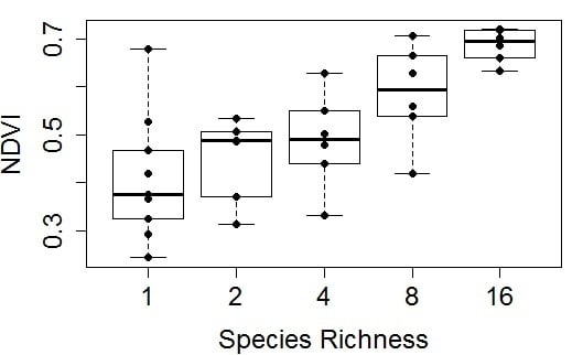
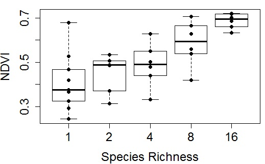
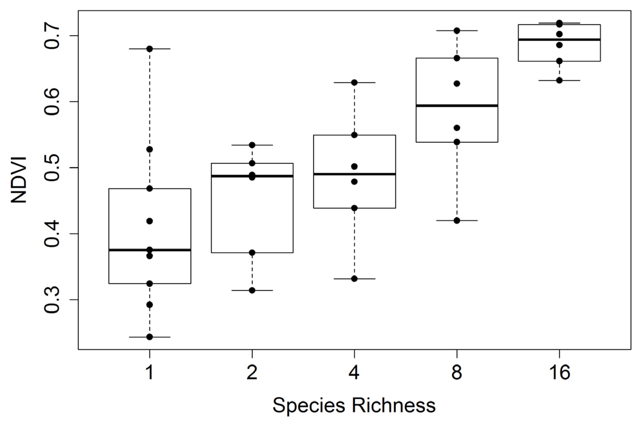
Figure 7.
Mid-season whole-plot NDVI
versus species richness (collected over several dates spanning 23 July to 3 August 2014). For this figure, 49 (7 m × 7 m) of the 81 measurements in the center of each plot were used to calculate the average reflectance and NDVI, yielding a more representative sampling than shown in
Figure 6. Species richness represents the planted number of species per plot. Each richness treatment had a sample size of 6, except monoculture plots, which had a sample size of 9. In this figure, box plots were overlaid on actual data points (dots) that represent the average values for each plot. The regression statistics are provided in
Table 2.
Table 2.
Species richness–NDVI relationships for various dates in 2014 compared to the whole plot results obtained at mid-summer (23 July–2 August 2014).
Table 2.
Species richness–NDVI relationships for various dates in 2014 compared to the whole plot results obtained at mid-summer (23 July–2 August 2014).
| Sampling | Regression Equation | R2 | p Value |
|---|
| 23 May | y = 0.0132x + 0.2821 | 0.2587 | 0.001 |
| 8 June | y = 0.0211x + 0.4841 | 0.3312 | 0.0003 |
| 20 June | y = 0.0199x + 0.548 | 0.3137 | 0.0005 |
| 06 July | y = 0.0193x + 0.5651 | 0.3325 | 0.0003 |
| 18 July | y = 0.0207x + 0.5022 | 0.374 | 9.51 × 10⁻⁵ |
| 4 August | y = 0.0178x + 0.3909 | 0.4728 | 5.04 × 10⁻⁶ |
| 21 August | y = 0.0157x + 0.4725 | 0.3789 | 0.0001 |
| 5 September | y = 0.0119x + 0.4957 | 0.2737 | 0.001 |
| 11 October | y = 0.0034x + 0.3854 | 0.05 | 0.209 |
| Whole-plot Sampling | y = 0.0177x + 0.4114 | 0.5136 | 6.07 × 10⁻⁷ |
A more complete summary of the effects of sample date and size on the NDVI-species richness relationship is provided in
Table 2, clearly illustrating that the strongest relationships were obtained towards mid-summer when plants were fully mature and before the onset of senescence, and that larger sample sizes based on whole-plot data improved the relationships. The seasonal pattern in the NDVI-species richness relationship (expressed as
R2 values) can be compared to the NDVI time trend, showing a peak in the correlation during the mid-season dip in NDVI, a time of warm, dry conditions and peak anthesis (
Figure 5 and
Figure 8).
Figure 8.
Time series of NDVI (black line) and R2 of the NDVI-species richness regression (red line) over the growing season in 2014. NDVI was the average value (±SEM) of all the plots on each sampling date.
Figure 8.
Time series of NDVI (black line) and R2 of the NDVI-species richness regression (red line) over the growing season in 2014. NDVI was the average value (±SEM) of all the plots on each sampling date.


