Multiscale Estimation of Leaf Area Index from Satellite Observations Based on an Ensemble Multiscale Filter

Abstract

Currently, multiple leaf area index (LAI) products retrieved from remote sensing data are widely used in crop growth monitoring, land-surface process simulation and studies of climate change. However, most LAI products are only retrieved from individual satellite observations, which may result in spatial-temporal discontinuities and low accuracy in these products. In this paper, a new method was developed to simultaneously retrieve multiscale LAI data from satellite observations with different spatial resolutions based on an ensemble multiscale filter (EnMsF). The LAI average values corresponding to the date of satellite observations were calculated from the multi-year Moderate Resolution Imaging Spectroradiometer (MODIS) LAI product and were used as a priori knowledge for LAI in order to construct an initial ensemble multiscale tree (EnMsT). Satellite observations obtained at different spatial resolutions were then applied to update the LAI values at each node of the EnMsT using a two-sweep filtering procedure. Next, the retrieved LAI values at the finest scale were used as a priori knowledge for LAI for the new round of construction and updating of the EnMsT, until the sum of the difference of LAI values at each node of the EnMsT between two adjacent updates is less than a given threshold. The method was tested using Thematic Mapper (TM) or Enhanced Thematic Mapper Plus (ETM+) surface reflectance data and MODIS surface reflectance data from five sites that have different vegetation types. The results demonstrate that the retrieved LAI values for each spatial resolution were in good agreement with the aggregated LAI reference map values for the corresponding spatial resolution. The retrieved LAI values at the coarsest scale provided better accuracy with the aggregated LAI reference map values (root mean square error (RMSE) = 0.45) compared with that obtained from the MODIS LAI values (RMSE = 1.30).

1. Introduction

Leaf area index (LAI) is defined as half of the total area of green leaves for a given unit of horizontal ground surface area [1]. LAI is an essential land surface biophysical parameter that describes the amount and change of vegetation, and is a significant input for climate and ecological simulations, including crop growth models [2], hydrological models [3], ecology models [4], weather forecasting [5] and studies of climate change [6].

Many methods have been developed to retrieve LAI from satellite remote-sensing data. In general, the methods used to estimate LAI from remote sensing data can be distinguished into two types: empirical methods and physical methods. Empirical methods, which utilize statistical relationships between LAI and a variety of vegetation indices to calculate LAI values, are easy to operate and are computational efficient [7,8]. However, the main limitation of these empirical methods is their dependence on measurement conditions, sites and vegetation types. Physical methods are based on the inversion of canopy radiative-transfer models to simulate physical and biological process and provide an explicit connection between canopy biophysical variables and the resulting canopy bidirectional reflectances. Since physical methods can be adjusted for a wide range of situations, an increasing number of studies tend to use canopy radiative-transfer models in the inversion of LAI values [9,10].

Currently, multiple global LAI products were generated from moderate resolution remote sensing data such as the Moderate-Resolution Imaging Spectroradiometer (MODIS) [11] and VEGETATION [12]. Several regional LAI products were also generated from high resolution satellite data (i.e., the Advanced Spaceborne Thermal Emission and Reflection Radiometer (ASTER) [13] and the Thematic Mapper (TM) [14]). These LAI products are routinely generated from remote-sensing data acquired only at a specific time. Because limited information is used for the inversion process, these products are not spatially and temporally continuous [15,16]. To obtain better retrieval results, some assimilation methods were developed to estimate LAI values from time-series satellite observations [17]. Xiao et al. [17] developed a temporally integrated inversion method by coupling a radiative-transfer model and a double-logistic model to estimate LAI values from time-series MODIS reflectance data. Jiang et al. [18] implemented a sequential assimilation method with an incremental analysis update to provide a smooth and continuous LAI time series from MODIS reflectance data. Lewis et al. [19] developed an Earth Observation Land Data Assimilation System (EO-LDAS) to improve the inversion of biophysical parameters. Viskari et al. [20] used ensemble adjustment Kalman filter (EAKF) to update predictions of LAI and leaf extension, which successfully simulated the evolution of plant leaf phenology and improved model predictions of forest net ecosystem exchange. All of these methods show the ability to retrieve temporally continuous LAI from reflectance data in time series. However, these methods only use individual satellite observations during the retrieval process.

To make full use of remote sensing information during the retrieval process, many data fusion methods, such as optimal interpolation (OI) [21], Bayesian maximum entropy (BME) [22], Bayesian hierarchical models [23], multi-resolution tree (MRT) [24] and an empirical orthogonal function (EOF) [25], have been developed to improve the accuracy and integrity of land-surface parameter products by integrating multi-source data. Among these data fusion methods, the MRT method has the advantage of integrating multi-resolution data with high computational efficiency and can generate products with different resolutions [26]. It has been used extensively to integrate soil moisture data [27], precipitation data [28] and land-surface albedo [29] from different satellite observations. To obtain spatially complete LAI products with different resolutions, Xiao et al. [24] integrated MODIS and ETM+ LAI via the MRT method. Wang et al. [30] also utilized the MRT method to fuse MODIS and Multi-angle Imaging SpectroRadiometer (MISR) LAI products with different resolutions.

To further improve computational efficiency and apply a nonlinear dynamic model via the MRT method, Zhou et al. [31] proposed an ensemble multiscale filter (EnMsF) method which combined the advantages of both the Ensemble Kalman Filter (EnKF) technique and the MRT method by adding state ensembles to the basic MRT method [32,33]. The EnMsF method has been applied in different fields, and some improvements have been made. Zhou [34] utilized the EnMsF method to estimate soil moisture and surface fluxes from multi-resolution L-band passive and active microwave soil moisture measurements following HYDROS specifications. Lawniczak et al. [35] applied the EnMsF method in reservoir engineering through assimilated permeability values and observations to obtain results at different scales. Pan et al. [36,37] developed an automated procedure for dividing irregular shapes to create a tree of “balanced” topology, and introduced the EnMsF method to hydrological land surface-driven applications. Some analysis on impacts of accuracy, spatial availability and assimilation frequency on the EnMsF method have also been discussed [38].

However, the observation operators used in all of the aforementioned EnMsF methods are linear. Therefore, these methods cannot be used to directly retrieve LAI values from satellite observations because the radiative transfer model, which is a non-linear relationship between LAI and surface reflectance data, is used as an observation operator. This paper aims to introduce the radiative transfer model into the EnMsF method to simultaneously retrieve multiscale LAI from satellite observations with different spatial resolutions.

An initial ensemble multiscale tree (EnMsT) is constructed with the LAI average values corresponding to the date of satellite observations calculated from the multi-year MODIS LAI product, and TM/ETM+ and MODIS reflectance data were used to update the LAI values at each node of the EnMsT by using a two-sweep filtering procedure. Then, the retrieved LAI values at the finest scale were used as a priori knowledge for LAI for the new round of construction and updating of the EnMsT, until the sum of the difference of LAI values at each node of the EnMsT between two adjacent updates is less than a given threshold. The retrieved LAI values with different resolutions were compared with LAI reference maps calculated from ground measurements at several sites with different vegetation types.

The organization of this paper is as follows. Section 2 provides the details of the method. The radiative-transfer model is first introduced, followed by the construction of the EnMsT. Then the two-sweep filtering procedure is described to retrieve LAI values from multi-resolution reflectance data. The satellite data products used in this study, and the LAI reference maps at the selected sites are also described in this section. Section 3 shows the performance of the new method and we provide an analysis of the retrieved results. Discussions are presented in Section 4, and the final section provides brief conclusions.

2. Methodology and Data

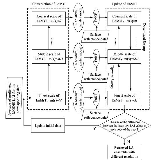
The general process of the new method to retrieve multiscale LAI data from satellite observations with different spatial resolutions is shown in Figure 1. The multi-year average of MODIS LAI corresponding to the date of satellite observations is used as a priori knowledge for LAI at the finest scale to construct an initial EnMsT. A two-sweep filtering procedure is used to update node states on the tree by integrating multiple satellite observations with different spatial resolutions. For the upward sweep, an EnKF was used to update the node states from satellite observations from the finest scale to the coarsest scale by coupling the EnMsT with a canopy radiative transfer model. The downward sweep starts from the coarsest scale and ends at the finest scale to smooth the node states on the tree according to all of the satellite observations. Then, the updated node states at the finest scale are used as the a priori knowledge for LAI for the new round of construction and updating of the EnMsT. The satellite observations are reused to update nodes states on the EnMsT by using the two-sweep filtering procedure. The circulation process will continue until the sum of the difference of LAI values at each node of the tree between two adjacent updates is less than a threshold, which is set to 0.01 in this study. Then, the ensemble mean of LAI at each node of the EnMsT for the last round was recorded as the retrieved LAI values at different resolutions.

2.1. Radiative-Transfer Model

Canopy radiative-transfer models describe the relationship between canopy reflectance and canopy characteristics. The two-layer canopy reflectance model (ACRM) developed by Kuusk [39,40] can be used for canopy reflectance modeling at spectral wavelengths ranging from 400 to 2400 nm. Many studies have used ACRM to retrieve biophysical parameters from satellite remote sensing data [41,42].

In this study, the latest version of ACRM was used to calculate the directional reflectance factor of vegetation canopies. The LAI of the lower layer was set to zero, or in other words, there was only one layer in the canopy. The parameters needed to run the ACRM are listed in

Table 1. Parameters needed to run the ACRM.

Parameters	Symbol	Values	Units
Leaf area index *	lai	0–10.0	m2/m2
The hot-spot parameter	sl	0.1	--
Foliage clumping parameter	clmp	0–2.0	--
The displacement parameter	szz	1.2	--
The elliptical leaf angle distribution	eln	2.0	--
Mean leaf angle of the LAD	thm	45.0	degree
Factor for refraction index	nratio	0.9	--
Leaf specific weight *	slw	80.0–180.0	g/m2
Leaf water content	c1	137.0	1/cm
Chlorophyll AB content *	c2	0.2–0.7	cm2/g
Leaf dry matter content	c3	98.0	cm2/g
Anthocyanin	c4	0.038	cm2/g
Leaf structure parameter	N	1.624	--
Weight of the first Price function *	s1	0.05–0.4	--
Weight of the Second Price function	s2	0.0	--
Weight of the third Price function	s3	0.0	--
Weight of the fourth Price function	s4	0.0	--

* Free parameters.

. Based on a global sensitivity analysis of the ACRM using an extension of the Fourier amplitude sensitivity testing (EFAST) [43,44], four parameters (lai, slw, c2, and s1) to which remote sensing signals are most sensitive were chosen as free variables in this study and are marked by asterisks in Table 1, and other nonsensitive parameters were set to empirical values.

2.2. Construction of the Ensemble Multiscale Tree

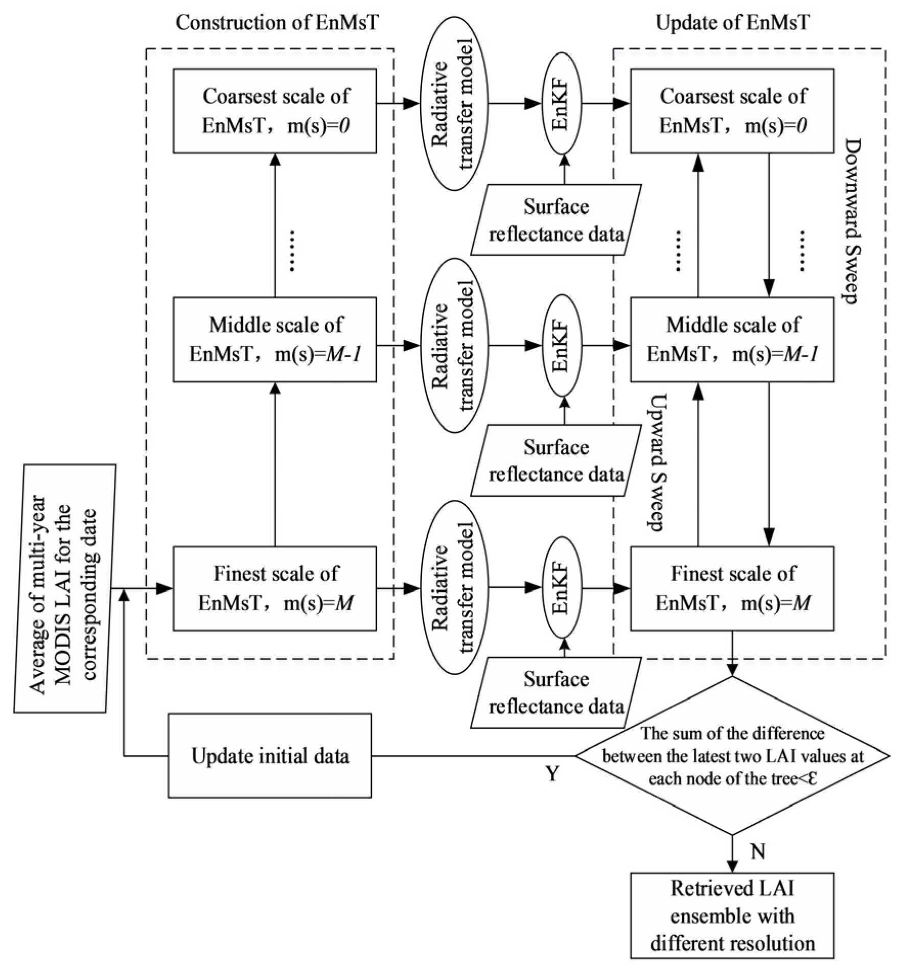
The EnMsT was first proposed by Zhou et al. [31], which is based on the original multiscale tree [32]. During the process of construct the tree, the global correlations are built up from local correlations between nearby tree nodes [31]. As shown in Figure 2, an ensemble multiscale tree is made up of a set of nodes. Let s be a node on the tree, $\mathit{\chi }\left(s\right)$ be a $n\left(s\right)$ dimension state vector at the node. We define a matrix $\mathit{x}\left(s\right)\in {\mathbf{\Re }}^{n\left(s\right)\times N}$ that contains N ensemble members of the state vector, namely $\mathit{x}\left(s\right)=\left({\mathit{\chi }}^1\left(s\right),{\mathit{\chi }}^2\left(s\right),\cdots ,{\mathit{\chi }}^N\left(s\right)\right)$. Except for nodes at the finest scale, all nodes on the tree have $q$ children $s{\alpha }_1,s{\alpha }_2,\cdots ,s{\alpha }_q$. Moreover, except for nodes at the coarsest scale, all nodes have a single parent $s\gamma$. Let $m\left(s\right)$ be the scale where node s is located. $m\left(s\right)$ increases from 0, which represents the top of the tree (i.e., the coarsest scale), to M, which represents the bottom of the tree (i.e., the finest scale). Nodes at the finest scale represent the highest resolution, while nodes at the coarsest scale represent the lowest resolution. From bottom to top, both the number of nodes and the spatial resolution at each scale are reduced proportionally. Inside the EnMsT, nodes at the same scale are not directly linked. Instead, each node is linked with its parent at the coarser scale and children at the finer scale. In Figure 2, this parent-child relationship among nodes is described using black solid lines.

According to the structure of the ensemble multiscale tree, different nodes at the finest scale are related through their common parent nodes [32]. Based on the multiscale autoregressive (MAR) model, the following state transition equations can be used to compute node states recursively across the tree [32,45]. The downward recursion transiting parent state to child state is:

$$\mathit{x}\left(s\right)=\mathit{A}\left(s\right)\mathit{x}\left(s\gamma \right)+\mathit{\omega }\left(s\right)$$

(1)

and the upward recursion transiting child state to parent state is:

$$\mathit{x}\left(s\gamma \right)=\mathit{F}\left(s\right)\mathit{x}\left(s\right)+{\mathit{\omega }}^{\prime }\left(s\right)$$

(2)

where $\mathit{A}\left(s\right)$ is a downward transition matrix and $\mathit{\omega }\left(s\right)$ is zero-mean random noise with covariance $\mathit{Q}\left(s\right)$, $\mathit{F}\left(s\right)$ is a upward transition matrix and ${\mathit{\omega }}^{\prime }\left(s\right)$ is zero-mean random noise with covariance ${\mathit{Q}}^{\prime }\left(s\right)$.

To get the scale transition and covariance matrices for all nodes at different scales, Frakt and Willsky [32] found that two conditions must be satisfied among nodes on the tree: one is the “locally internal” condition, and the other one is the “scale-recursive Markov property”. The “locally internal” condition means that the parent state $\mathit{x}\left(s\right)$ is a linear combination of all its children’s states ${\mathit{x}}_{m\left(s\right)+\mathbf{1}}\left(s{\alpha }_i\right)$. Thus the ensemble version can be written as:

$$\mathit{x}\left(s\right)=\mathit{V}\left(s\right){\mathit{x}}_{m\left(s\right)+\mathbf{1}}\left(s\right)=\mathit{V}\left(s\right)\left[\begin{array}{c}\mathit{x}\left(s{\alpha }_1\right)\\ ⋮\\ \mathit{x}\left(s{\alpha }_q\right)\end{array}\right],m\left(s\right)<M$$

(3)

where $\mathit{x}\left(s{\alpha }_1\right),\mathit{x}\left(s{\alpha }_2\right),\cdots ,\mathit{x}\left(s{\alpha }_q\right)$ are $q$ state vectors at children nodes $s{\alpha }_i$, and $\mathit{V}\left(s\right)$ is a coefficient matrix with a dimension of $n\left(s\right)\times \left(qn\left(s\alpha \right)\right)$. The “scale-recursive Markov property” means that for any node located at scale $m\left(s\right)(m\left(s\right)<M)$, its state $\mathit{x}\left(s\right)$ is conditionally uncorrelated with these $q+1$ sets. Based on these two properties, the maximum predictive efficiency method, which is described in detail in Willsky [45] and Zhou [34], is used to calculate the coefficient matrix $\mathit{V}\left(s\right)$. Then it is easy to determine the scale transition and covariance matrices for all nodes at different scales:

$$\mathit{A}\left(s\right)=\text{cov}\left[\mathit{x}\left(s\right),\mathit{x}\left(s\gamma \right)\right]{\text{cov}}^{-1}\left[\mathit{x}\left(s\gamma \right)\right]$$

(4)

$$\mathit{F}\left(s\right)=\text{cov}\left[\mathit{x}\left(s\gamma \right)\right]\mathit{A}{\left(s\right)}^{\mathrm{T}}{\text{cov}}^{-1}\left[\mathit{x}\left(s\right)\right]$$

(5)

$$\mathit{Q}\left(s\right)=\text{cov}\left[\mathit{x}\left(s\right)\right]-\mathit{A}\left(s\right)\text{cov}{\left[\mathit{x}\left(s\right),\mathit{x}\left(s\gamma \right)\right]}^{\mathrm{T}}$$

(6)

$${\mathit{Q}}^{\prime }\left(s\right)=\text{cov}\left[\mathit{x}\left(s\gamma \right)\right]-\mathit{F}\left(s\right)\mathit{A}\left(s\right)\text{cov}\left[\mathit{x}\left(s\gamma \right)\right]$$

(7)

In this study, the four free variables from the ACRM, which are denoted by asterisks in Table 1, were included in each node state $\mathit{x}\left(s\right)$. As such, the size of the node state vector $n\left(s\right)$ is equal to four. The average and standard deviation of multi-year MODIS LAI product corresponding to the date of satellite observations was used as a priori knowledge for LAI at the finest scale to construct the initial EnMsT. The scale transition matrices and covariance matrices at each node of the EnMsT were calculated according to the formulas above.

2.3. Updating the Ensemble Multiscale Tree

When finishing the construction of the EnMsT, satellite observations with different spatial resolutions were used to update the LAI values at each node of the EnMsT. The updating procedure can be divided into two steps: an upward sweep and a downward sweep.

2.3.1. Upward Sweep

For each node of the EnMsT, the upward sweep procedure updates the state vector from satellite observations using an EnKF technique. The EnKF uses an ensemble of model states to represent the statistical errors, and then uses ensemble integrations to forecast these errors forward during the model estimation [33]. The EnKF analysis equation is as follows:

$${\mathit{\chi }}^{\mathit{j}}\left(s|s\right)={\mathit{\chi }}^{\mathit{j}}\left(s\right)+\mathit{K}\left(s\right)\left[{\mathit{Y}}^{\mathit{j}}\left(s\right)-{\mathit{Y}}^{\prime \mathit{j}}\left(s\right)\right]$$

(8)

where ${\mathit{\chi }}^{\mathit{j}}\left(s|s\right)$ is a state vector after an upward update; ${\mathit{\chi }}^{\mathit{j}}\left(s\right)$ is an initial state vector; ${\mathit{Y}}^{\mathit{j}}\left(s\right)$ is a perturbed observation vector, which is composed of satellite observations of current node and the states of its children nodes; and ${\mathit{Y}}^{\prime \mathit{j}}\left(s\right)$ is a vector which contains the simulated satellite observations and the predicted states of children nodes from the current node. The detailed calculation function was written in Zhou et al. [31]. $\mathit{K}\left(s\right)$ is a Kalman gain and can be written as:

$$\mathit{K}\left(s\right)=\text{cov}\left[\mathit{x}\left(s\right),{\mathit{Y}}^{\prime }\left(s\right)\right]{\left\{\text{cov}\left[{\mathit{Y}}^{\prime }\left(s\right)\right]+\mathit{R}\left(s\right)\right\}}^{-1}$$

(9)

where $\text{cov}\left[\mathit{x}\left(s\right),{\mathit{Y}}^{\prime }\left(s\right)\right]=E\left\{\left[\mathit{x}\left(s\right)-E\left(\mathit{x}\left(s\right)\right)\right]{\left[{\mathit{Y}}^{\prime }\left(s\right)-E\left({\mathit{Y}}^{\prime }\left(s\right)\right)\right]}^{\mathrm{T}}\right\}$ and $\text{cov}\left[{\mathit{Y}}^{\prime }\left(s\right)\right]$ is short for $\text{cov}\left[{\mathit{Y}}^{\prime }\left(s\right),{\mathit{Y}}^{\prime }\left(s\right)\right]=E\left\{\left[{\mathit{Y}}^{\prime }\left(s\right)-E\left({\mathit{Y}}^{\prime }\left(s\right)\right)\right]{\left[{\mathit{Y}}^{\prime }\left(s\right)-E\left({\mathit{Y}}^{\prime }\left(s\right)\right)\right]}^{\mathrm{T}}\right\}$; $\mathit{R}\left(s\right)$ is an observation error covariance matrix; and the superscript “$\mathrm{T}$” denotes a matrix transpose.

Equation (8) imposes the condition that the observation operator $\mathit{h}\left(·\right)$ is linear, ${\mathit{Y}}^{\prime \mathit{j}}\left(s\right)= \mathit{h}\left(s\right){\mathit{\chi }}^{\mathit{j}}\left(s\right)$. Therefore, Equation (8) becomes invalid when satellite observations are used to update the node states on the EnMsT because the canopy radiative transfer model represents a non-linear function of node states. To overcome this limitation, the state vector ${\mathit{\chi }}^{\mathit{j}}\left(s\right)$ can be augmented with a diagnostic variable from observations simulated by the canopy radiative transfer model [46]. Therefore, a new state vector is defined as ${\widehat{\mathit{\chi }}}^{\mathit{j}}\left(s\right)=\left[{\mathit{\chi }}^{\mathit{j}\mathrm{T}}\left(s\right),{\mathit{h}}^{\mathrm{T}}\left({\mathit{\chi }}^{\mathit{j}}\left(s\right)\right)\right]\in {\mathbf{\Re }}^{\widehat{n}\left(s\right)}$ with $\widehat{n}\left(s\right)$ being the sum of the dimension of the node state vector $n\left(s\right)$ and the number of measurement equivalents. Thus the new update equation is:

$${\mathit{\chi }}^{\mathit{j}}\left(s|s\right)={\mathit{\chi }}^{\mathit{j}}\left(s\right)+\widehat{\mathit{K}}\left(s\right)\left[{\mathit{Y}}^{\mathit{j}}\left(s\right)-\widehat{\mathit{H}}{\widehat{\mathit{\chi }}}^{\mathit{j}}\left(s\right)\right]$$

(10)

where $\widehat{\mathit{H}}$ is a linear observation operator that relates the augmented state vector to satellite observations, and $\widehat{\mathit{K}}\left(s\right)$ is the new Kalman gain:

$$\widehat{\mathit{K}}\left(s\right)=\text{cov}\left[\mathit{x}\left(s\right),{\widehat{\mathit{Y}}}^{\prime }\left(s\right)\right]{\left\{\text{cov}\left[{\widehat{\mathit{Y}}}^{\prime }\left(s\right)\right]+\mathit{R}\left(s\right)\right\}}^{-1}$$

(11)

During the upward sweep procedure, the node states on the tree are updated using the EnKF technique from the finest scale to the coarsest scale. For each node at the finest scale, only satellite observations were used to update the state at this node. If no satellite observation exists, the update just comes from the state of the node itself. However, for each node located above the finest scale, the observations used to update the state at this node include data obtained by satellites as well as the states of its children nodes. If there is no satellite observation, the node is updated according to the states of its children nodes.

2.3.2. Downward Sweep

After the upward sweep, the downward sweep is conducted from the top to the bottom of the tree. During this process, nodes are smoothed from the top down depending on all of the satellite observations on the EnMsT.

If node s is located at the top of the tree, the state vector after a downward sweep ${\mathit{\chi }}^{\mathit{j}}\left(s|S\right)$ is kept the same as the state vector after the upward sweep [31]:

$${\mathit{\chi }}^{\mathit{j}}\left(s|S\right)={\mathit{\chi }}^{\mathit{j}}\left(s|s\right),m\left(s\right)=0$$

(12)

If node s is below the root node, the state vector after a downward sweep is:

$${\mathit{\chi }}^{\mathit{j}}\left(s|S\right)={\mathit{\chi }}^{\mathit{j}}\left(s|s\right)+\mathit{J}\left(s\right)\left[{\mathit{\chi }}^{\mathit{j}}\left(s\gamma |S\right)-{\mathit{\chi }}^{\mathit{j}}\left(s\gamma |s\right)\right],m\left(s\right)>0$$

(13)

where ${\mathit{\chi }}^{\mathit{j}}\left(s\gamma |s\right)$ and ${\mathit{\chi }}^{\mathit{j}}\left(s\gamma |S\right)$ are the state vector of the parent node $s\gamma$ before and after the downward sweep, respectively, and $\mathit{J}\left(s\right)$ is the smoothing gain. ${\mathit{\chi }}^{\mathit{j}}\left(s\gamma |s\right)$ can be got from the MAR upward recursion in Equation (2) [31]:

$${\mathit{\chi }}^{\mathit{j}}\left(s\gamma |s\right)=\mathit{F}\left(s\right){\mathit{\chi }}^{\mathit{j}}\left(s|s\right)+{\mathit{\omega }}^{\prime j}\left(s\right)$$

(14)

and $\mathit{J}\left(s\right)$ is calculated as follow:

$$\mathit{J}\left(s\right)=\text{cov}\left[\mathit{x}\left(s|s\right)\right]{\mathit{F}}^{\mathrm{T}}\left(s\right){\text{cov}}^{-1}\left[\mathit{x}\left(s\gamma |s\right)\right]$$

(15)

After the two-sweep filtering procedure, the updated states of each node at different scales are recorded separately.

2.4. Data and Preprocessing

TM/ETM+ and MODIS surface reflectance data were used to test the new method at five sites from Bigfoot and Valeri: Bondville, Sud-Ouest, Laprida, Zhangbei, and Puechabon. Characteristics of these sites are given in

Table 2. Characteristics of the selected sites.

Site Name	Latitude (°)	Longitude (°)	Land Cover Type	Date of LAI Reference Maps (Day/Year)
Bondville	40.004	−88.29	Cropland	224/2000
Sud-Ouest	43.506	1.2375	Cropland	201/2002
Laprida	−36.990	−60.552	Grassland	317/2002
Zhangbei	41.278	114.687	Grassland	235/2002
Puechabon	43.724	3.651	Evergreen broadleaf forest	163/2001

.

The MODIS surface reflectance product (MOD09A1) from the latest version (Collection 5) and the Landsat 4–5 TM or Landsat 7 ETM+ surface reflectance data were inputted into the new method to simultaneously retrieve multiscale LAI data using the EnMsF. The MOD09A1 product, in a sinusoidal projection system, provided the surface reflectance for each of the MODIS land spectral bands. The spatial resolution was 500 m, and the temporal sampling period was 8 days. The surface reflectance data were contaminated by residual clouds or undetected cloud shadows. According to the product quality information, only reflectance data with the highest quality of all bands (QA = 0) were used in this paper. According to the typical theoretical uncertainties in the MODIS surface-reflectance product, the following values were assigned to the uncertainties in the MODIS surface reflectance: ±(0.005 + 0.05 × surface reflectance) [47]. The TM/ETM+ surface reflectance data were generated from the Landsat Ecosystem Disturbance Adaptive Processing System (LEDAPS) [48], with 30-m spatial resolution in a Universal Transverse Mercator (UTM) projection system. According to its quality control information, only pixels without clouds, cloud shadows, snow, or water (Cfmask = 0) were used. Furthermore, 5% of surface reflectance was assigned to the uncertainties in the TM/ETM+ surface reflectance data.

Considering the spatial resolutions of the MODIS and TM/ETM+ surface reflectance data, an EnMsT in which each node has four children is used in this study. The EnMsT has six different scales. The nodes at the coarsest scale (the 0th scale) have a spatial resolution of 926.6 m, while the nodes at the finest scale (the 5th scale) have a spatial resolution of 28.9 m. The nodes at intermediate scales have spatial resolutions of 463.3 m, 231.7 m, 115.8 m and 57.9 m, respectively. Therefore, the TM/ETM+ surface reflectance data were resampled to a spatial resolution of 28.9 m, which corresponds to the finest scale, and the MODIS surface reflectance data were reprojected to the UTM projection and resampled to a spatial resolution of 463.3 m, which corresponds to the 1st scale using the nearest-neighbor resampling method. In this study, the MODIS Collection 5, 8-day, 1-km LAI product (MOD15A2) from 2000 to 2010 was used to calculate the LAI average values corresponding to the date of satellite observations which were used as a priori knowledge for LAI at the finest scale to construct the initial EnMsT. The MODIS LAI data were also reprojected to the UTM projection and resampled to a spatial resolution of 926.6 m in order that they could be compared with the retrieved LAI at the 0 scale.

In addition, high resolution LAI reference maps at the selected sites were used to evaluate the accuracy and consistency of the LAI values retrieved by the new method. At the Bondville site, LAI ground measurements were measured using destructive sampling methods. The Landsat ETM+ imagery was used to develop high resolution LAI estimates, which are directly linked to ground measurements using the methods described by Gower et al. [49]. The high resolution LAI reference map has a spatial resolution of 25 m and covers a 7 km × 7 km region centered on the location of the site. Estimates of error in the regression predictions were obtained using cross-validation. For the Sud-Ouest, Laprida, Zhangbei and Puechabon sites, LAI ground measurements were calculated from digital hemispherical images using the method proposed by Lang and Yueqin [50]. The high-resolution LAI reference maps were derived from the determination of the transfer function between the reflectance values of the SPOT images acquired during the ground campaign and the LAI ground measurements [51]. The LAI reference maps of the four sites have a spatial resolution of 20 m, and each LAI reference map covers a 3 km × 3 km region centered on the location of the site. The accuracy of these LAI reference maps depends on ground measurement errors, uncertainties of high-resolution reflectance data, and sampling and upscaling errors [52]. Fernandes et al. [53] demonstrated that an absolute uncertainty smaller than 1 LAI unit can be expected. To evaluate the accuracy of the retrieved LAI with different spatial resolutions, the high resolution LAI reference map for each selected site was aggregated to the corresponding spatial resolutions using a spatial-average method.

3. Results

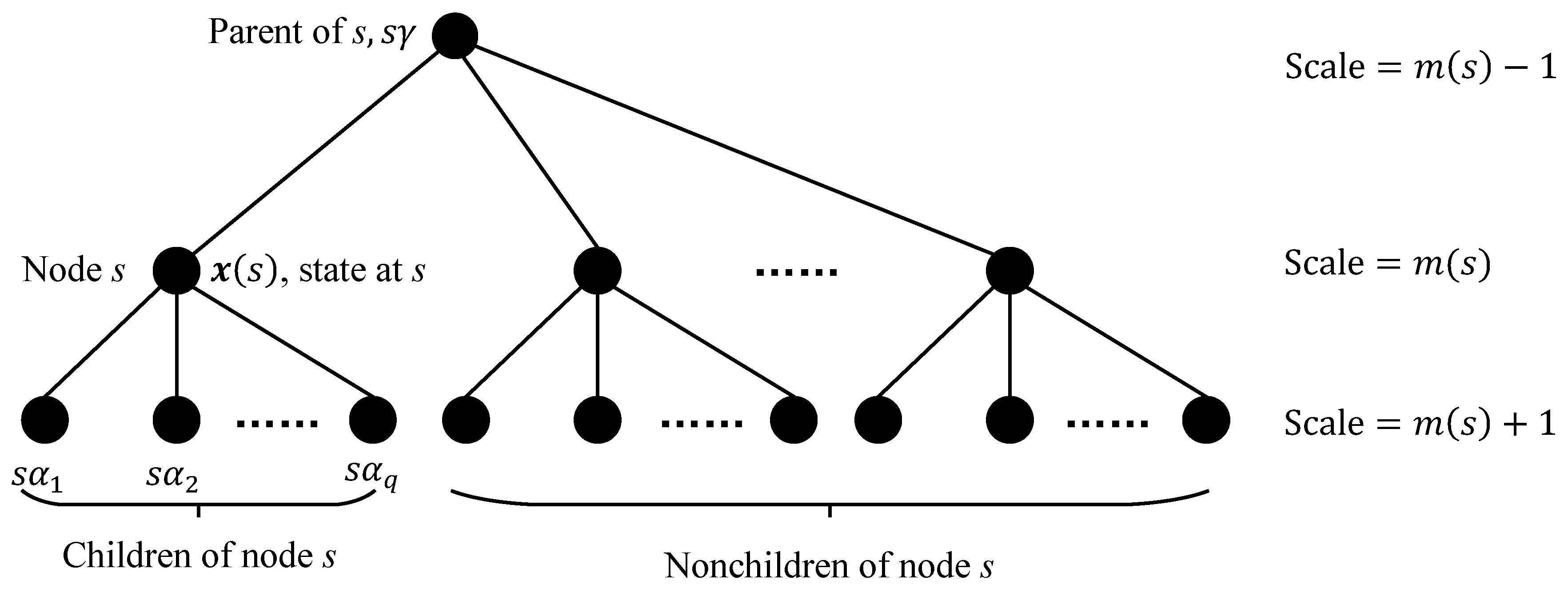
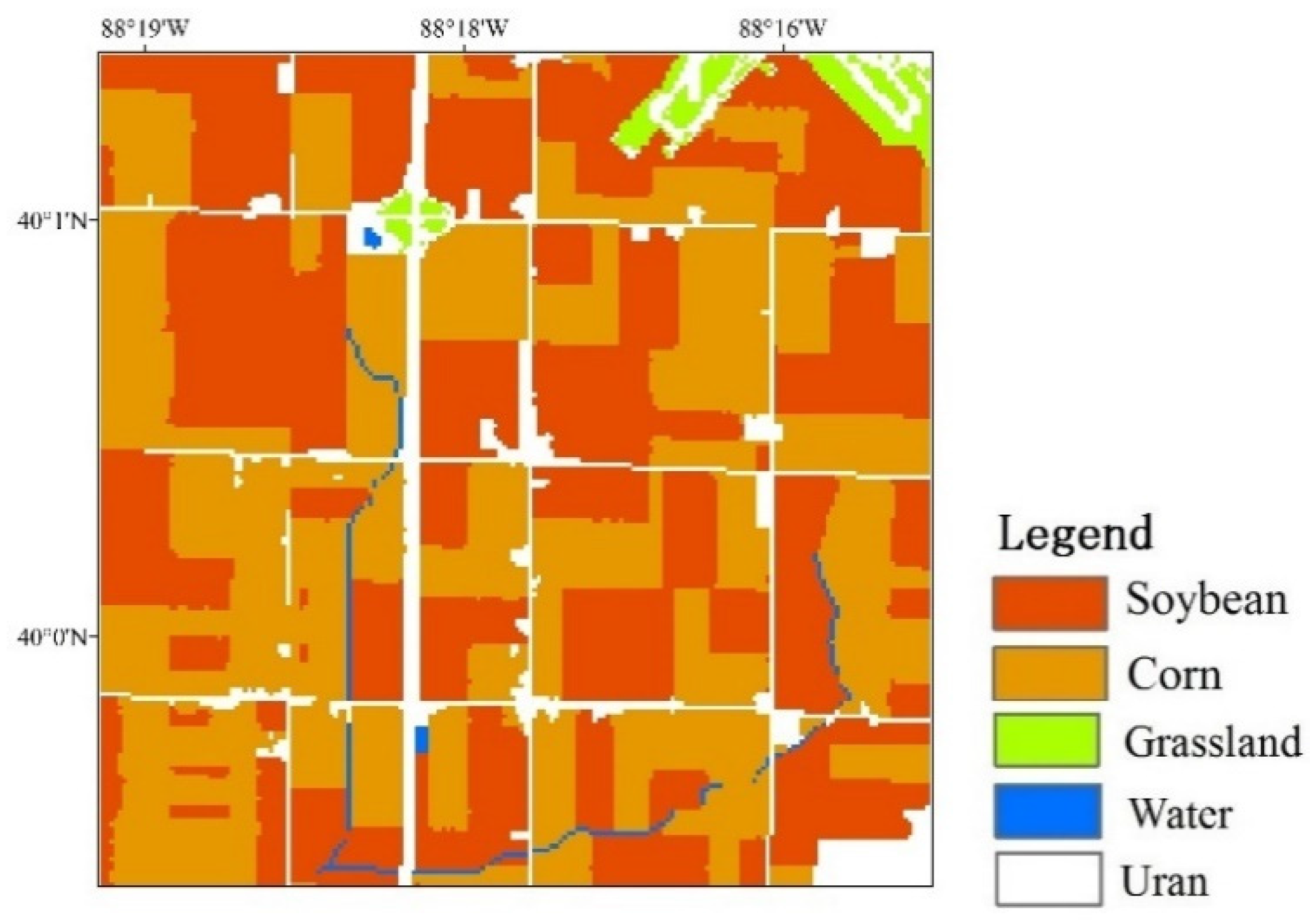
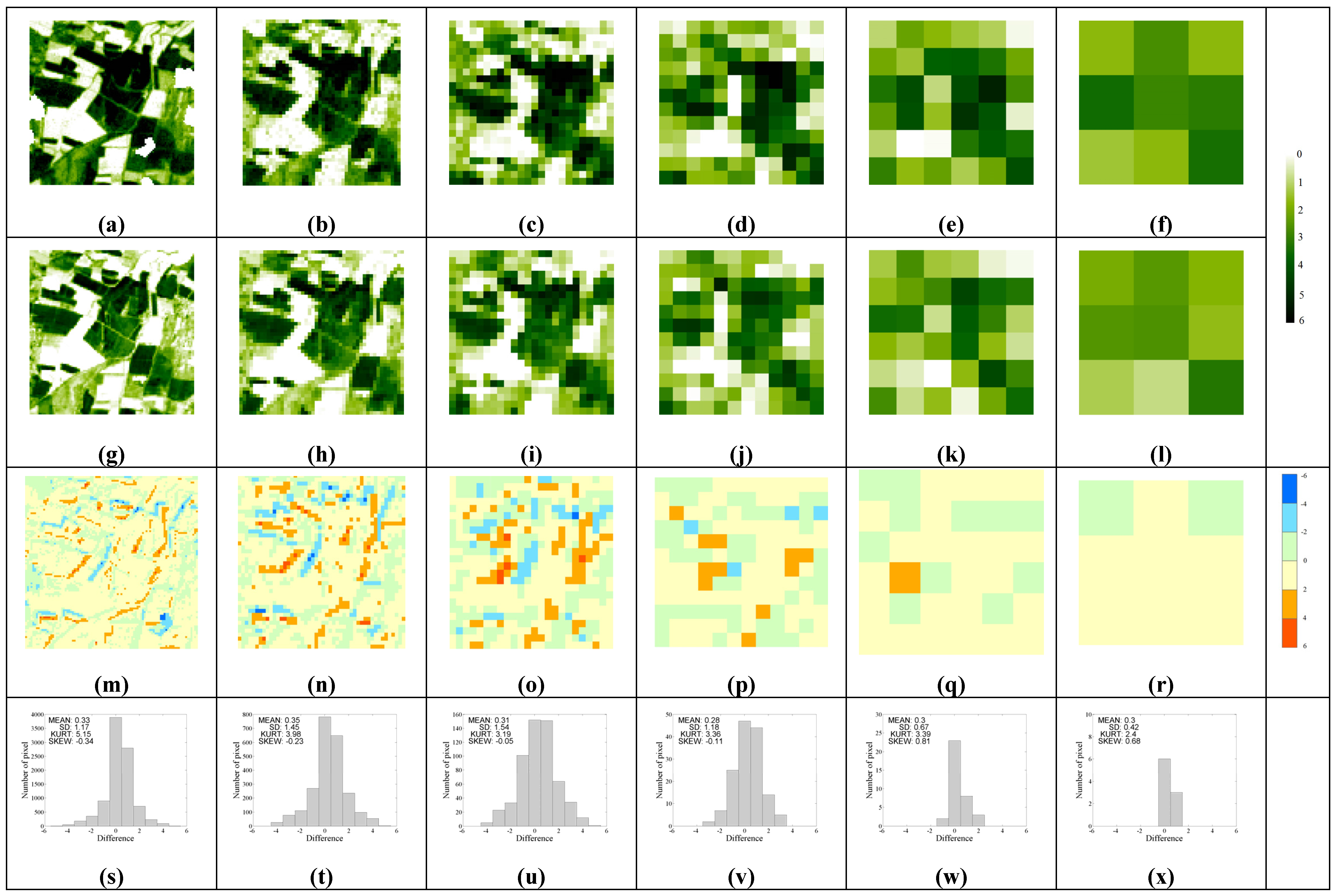
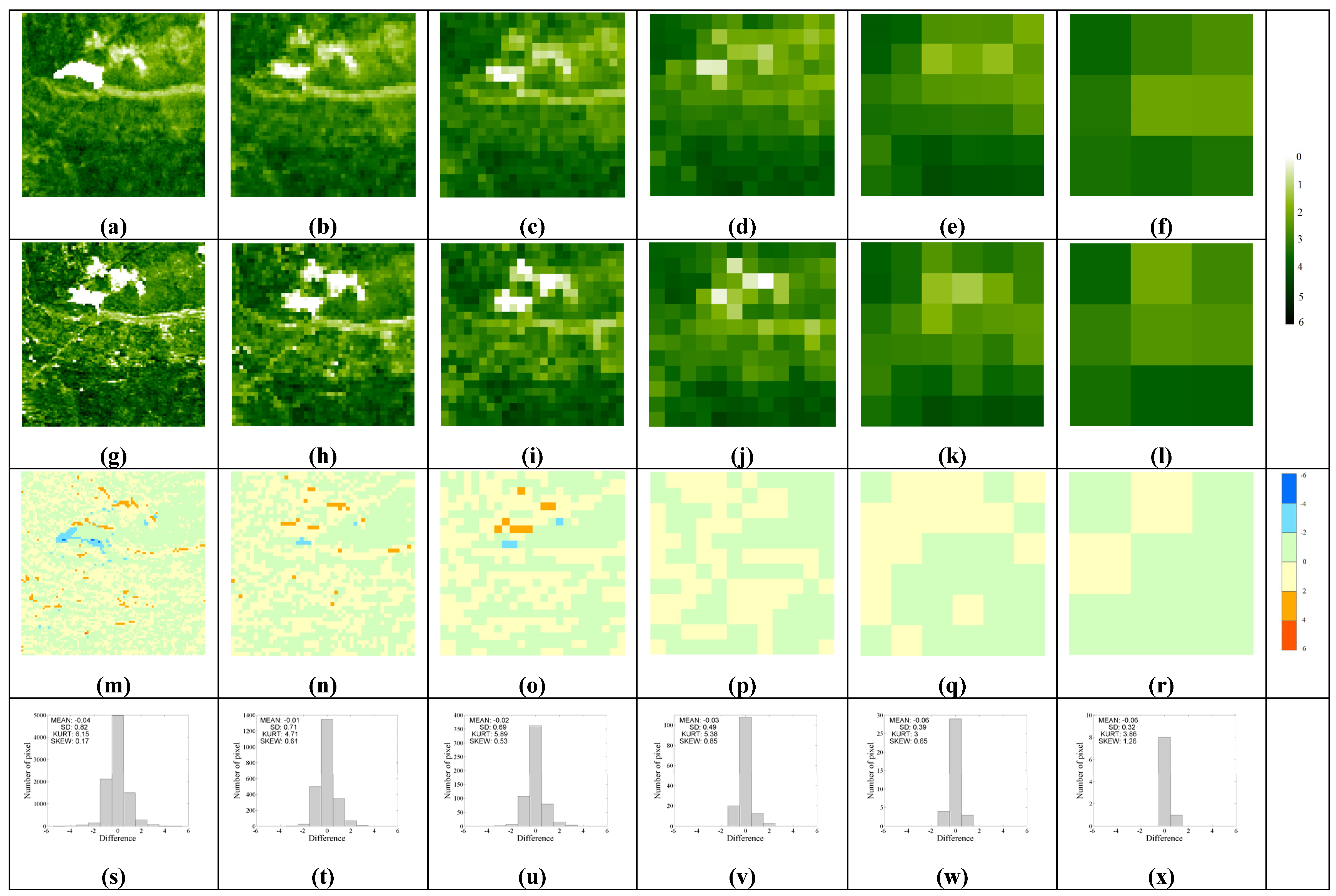
At the Bondville site, TM surface reflectance data obtained on Day 228, 2000 and MODIS surface reflectance data obtained on Day 225, 2000 were used to retrieve multiscale LAI values. The upper row in Figure 3 shows the maps of the retrieved LAI at spatial resolutions of 28.9 m, 57.9 m, 115.8 m, 231.7 m, 463.3 m, and 926.6 m, respectively. A land cover map at the Bondville site is shown in Figure 4. The site is an agricultural district where the main crops are soybeans and corn [54]. The maps of retrieved LAI show very consistent spatial patterns with the land cover map at this site.

To compare the retrieved LAI values at different scales, the aggregated LAI reference maps for each corresponding spatial resolution are shown in the second row of Figure 3. At each scale, the retrieved LAI values and LAI reference map values are in good agreement, especially in the central part. However, some differences exist in the western and eastern areas where the retrieved LAI values are slightly over-estimated relative to the LAI reference map values.

The last two rows of Figure 3 present the difference maps between the retrieved LAI and the aggregated LAI reference map for each corresponding spatial resolution and the frequency histograms. Seen from the difference map, the main difference between the retrieved LAI and the aggregated LAI reference map are mainly from the corn. For retrieved results, the average of retrieved LAI values of corn (approximately 6.5) is significantly higher than those of the soybeans (approximately 4.2). However, for the aggregated LAI reference map, the differences between LAI values of corn and soybeans are relatively small. Seen from the frequency histograms, it is observed that the LAI differences for most pixels at this site are concentrated around 0 at each spatial resolution. The positive mean values of LAI differences indicate that the retrieved LAI values are slightly higher than the LAI reference map values. The LAI differences at the finest scale have the largest standard deviation (Figure 3m). As the spatial resolution of the differences decreases, the standard deviation of LAI differences also gradually decreases.

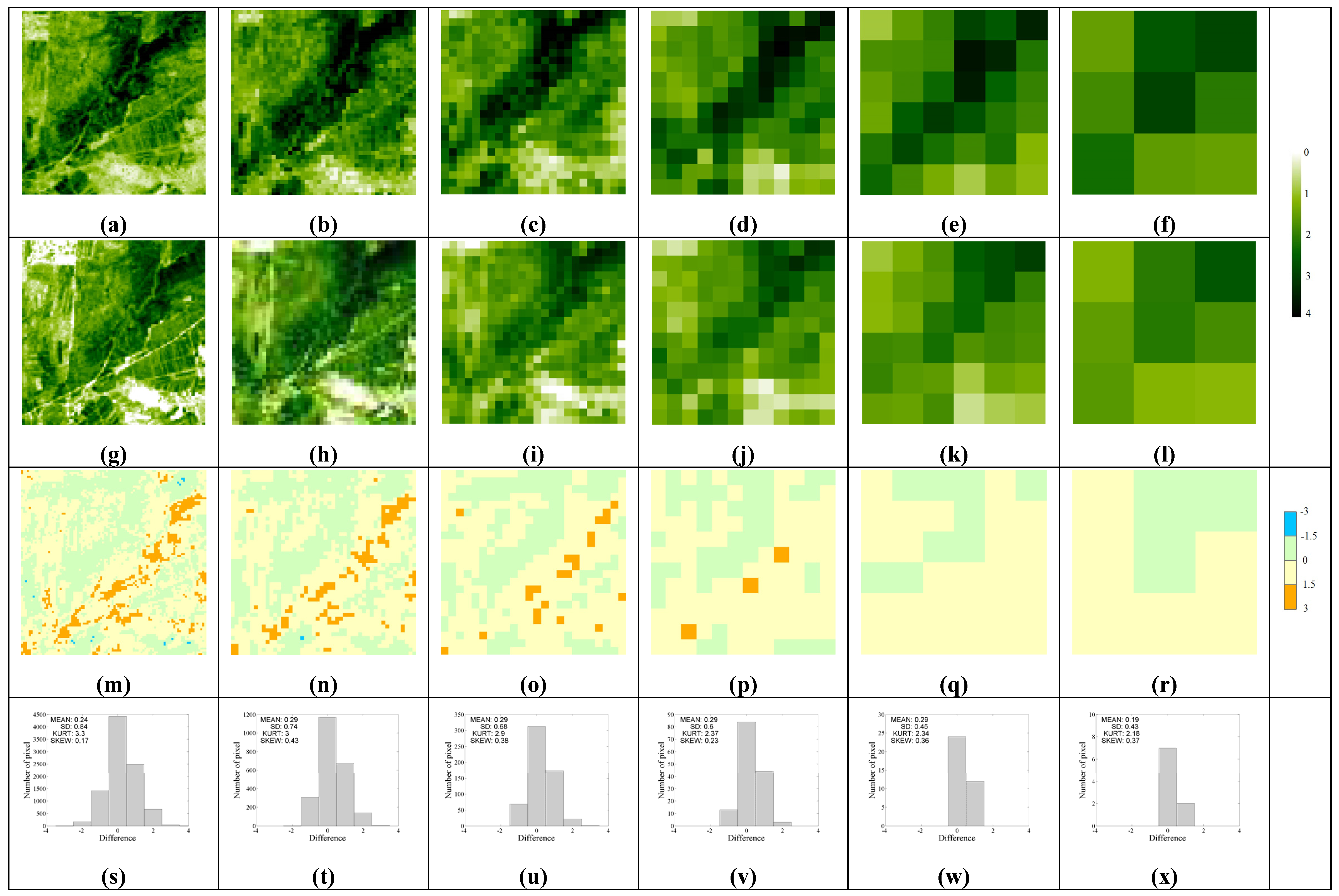
At the Sud-Ouest site, ETM+ surface reflectance data obtained on Day 203, 2002 and MODIS surface reflectance data obtained on Day 201, 2002 were utilized to retrieve multiscale LAI values. Maps of the retrieved LAI values at different spatial resolutions and the aggregated LAI reference maps are displayed in the upper and second row of Figure 5, respectively. The main land cover type at this site is cropland, including corn, soybeans and sunflowers [55]. The distribution of cropland can be clearly distinguished from the map of retrieved LAI values at the spatial resolution of 28.9 m. The retrieved LAI values can reflect the different growth conditions among the fields. It is apparent that maps of the retrieved LAI values and the aggregated LAI reference maps at each spatial resolution are generally consistent in their spatial patterns. However, the retrieved LAI values in the central area are close to 6.0, and are slightly higher than those from the aggregated LAI reference maps.

The difference maps between the retrieved LAI and the aggregated LAI reference map for each corresponding spatial resolution and the frequency histograms (shown in the lower row of Figure 5) demonstrate that the retrieved LAI values and the aggregated LAI reference map values were in good agreement at this site. The retrieved LAI values were slightly larger than the aggregated LAI reference map values and the mean values of LAI differences for each corresponding spatial resolution were less than 0.35.

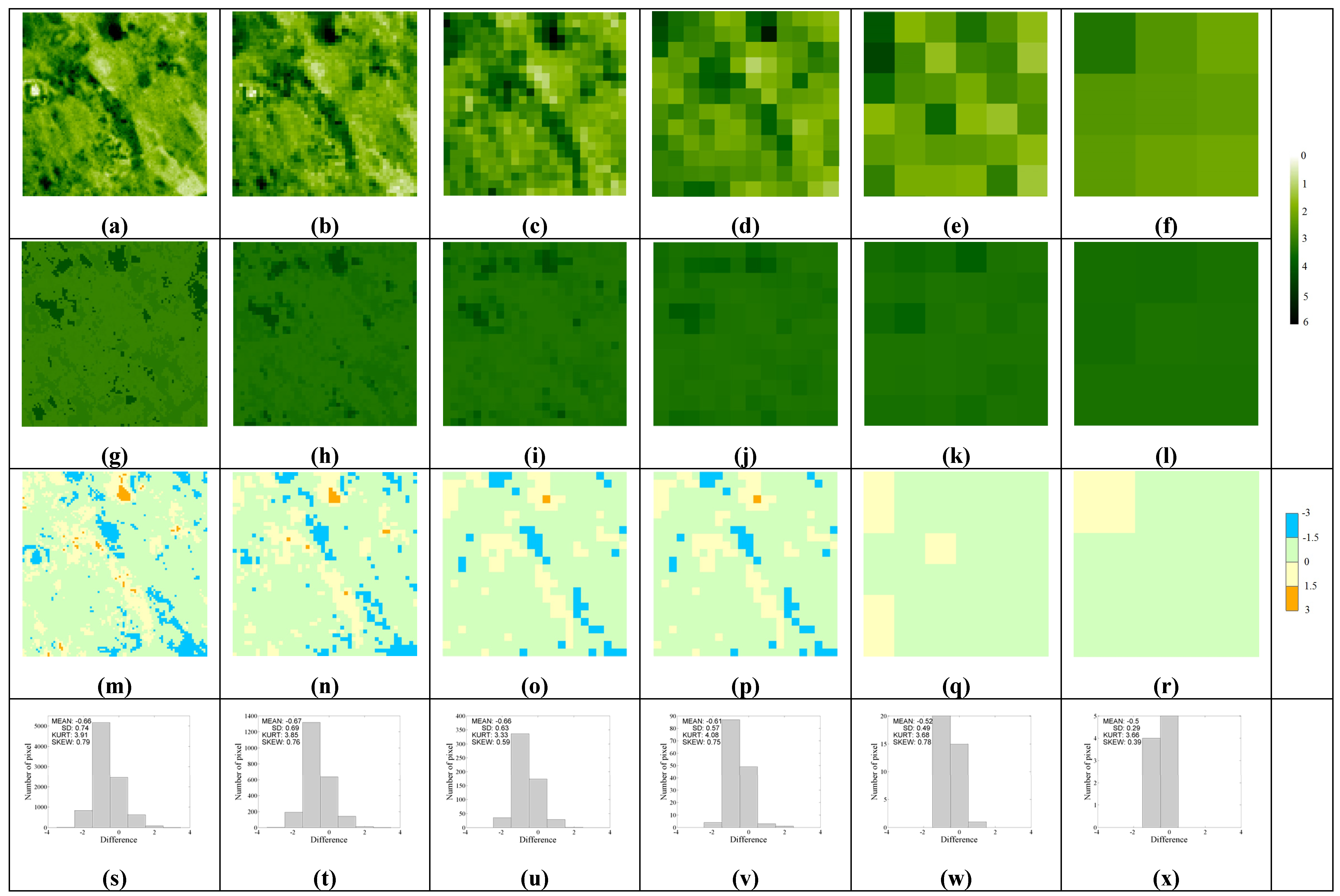
At the Laprida site, ETM+ surface reflectance data obtained on Day 328, 2002 and MODIS reflectance data obtained on Day 313, 2002 were utilized to retrieve multiscale LAI values. Maps of the retrieved LAI values at spatial resolutions of 28.9 m, 57.9 m, 115.8 m, 231.7 m, 463.3 m, and 926.6 m are shown in the upper row of Figure 6. For comparison, the aggregated LAI reference maps for the corresponding spatial resolutions were also shown in the second row of Figure 6. Compared with the aggregated LAI reference map values, the retrieved LAI values have a larger, dynamically changing range. More detailed information of the status of vegetation growth is demonstrated in the retrieved LAI values. However, for the LAI reference map at the finest scale, there are only two LAI values over the 3 km × 3 km area. As such, it is hard to reflect the discrepancies in LAI values among different land cover types from the LAI reference maps.

The lower row of Figure 6 shows the difference maps between the retrieved LAI and the aggregated LAI reference map for each corresponding spatial resolution and the frequency histograms at the Laprida site. Most pixels are centered on −0.6, and range from −1.5 to −0.5 with a comparatively high skewness (around 0.6). The difference maps also demonstrates that the retrieved LAI values for most pixels are lower than those from the LAI reference map values.

At the Zhangbei site, TM surface reflectance data obtained on Day 228, 2002 and MODIS surface reflectance data obtained on Day 233, 2002 were utilized to retrieve multiscale LAI values. Maps of the retrieved LAI values at different spatial resolutions, and the aggregated LAI reference maps are shown in the upper and second row of Figure 7, respectively. The retrieved LAI values were overestimated relative to the LAI reference map values at the northeast corner of these maps. the difference maps between the retrieved LAI and the aggregated LAI reference map for each corresponding spatial resolution and the frequency histograms (shown in the lower row of Figure 7) demonstrate that the retrieved LAI values were in excellent agreement with the aggregated LAI reference map values at this site. However, for some parts, the retrieved LAI values for most pixels are slightly higher than the aggregated LAI reference map values.

At the Puechabon site, ETM+ surface reflectance data obtained on Day 177, 2002 and MODIS surface reflectance data obtained on Day 161, 2002 were utilized to retrieve multiscale LAI values. Maps of the retrieved LAI values at different spatial resolutions and the aggregated LAI reference maps are shown in the upper and second row of Figure 8, respectively. It can be observed that pixels with the retrieved LAI values ranging from five to six are mainly distributed in the southern area of the maps where the vegetation type is forest. Pixels with grassland biomes are mainly distributed in the northern area of the maps and show lower LAI values.

The difference maps between the retrieved LAI and the aggregated LAI reference map for each corresponding spatial resolution and the frequency histograms (shown in the lower row of Figure 8) demonstrate that the retrieved LAI values and the aggregated LAI reference map values are in good agreement at this site. More than half of all pixels are centered on zero, and range from −0.5 to 0.5. Relatively high kurtosis exists at most scales, which also shows that there are very few discrepancies between the retrieved LAI values and the aggregated LAI reference map values.

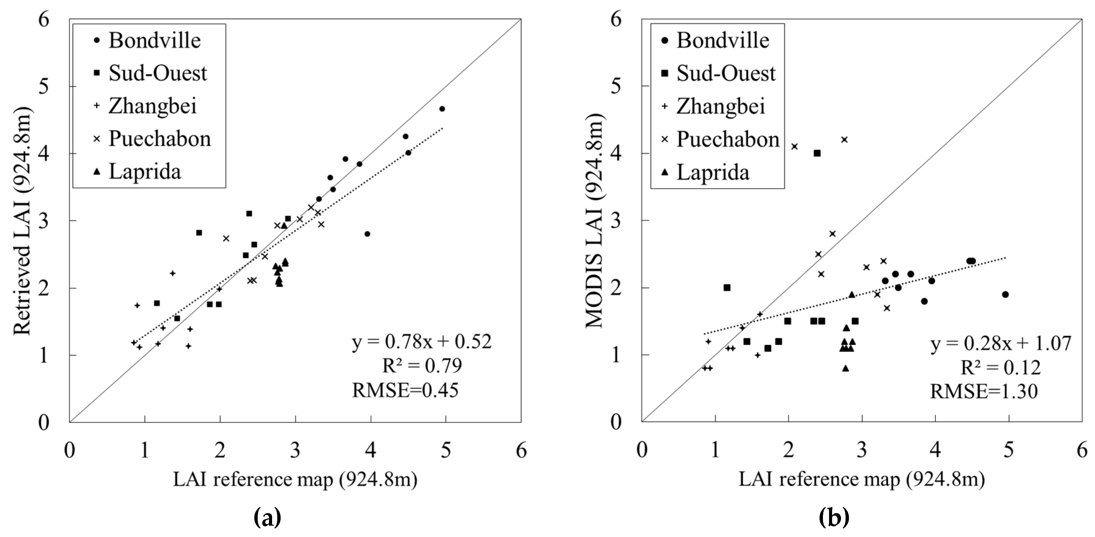
Figure 9 shows scatter plots of the retrieved LAI values at the coarsest scale and the MODIS LAI values versus the aggregated LAI reference map values at the corresponding spatial resolution over all the selected sites in Table 2. For each site, the MODIS LAI data that are closest to the date of the corresponding LAI reference map were selected for comparison. Compared with the MODIS LAI values, the retrieved LAI values in this study are distributed more closely around the 1:1 line with the aggregated LAI reference map values, which demonstrates that the retrieved LAI values achieved better agreement with the aggregated LAI reference map values across the whole range of LAI values than the MODIS LAI values. The regressions presented in Figure 9b show a positive intercept (1.07) and a slope smaller than one (0.28), indicating a systematically low bias in the MODIS retrievals at the selected sites with high LAI values, a result that is in agreement with the findings of Pisek and Chen [56]. Most of the scatters below the 1:1 line in Figure 9b belong to the Bondville, Sud-Ouest and Laprida sites. The retrieved LAI values in this study provide better accuracy with the aggregated LAI reference map values (RMSE = 0.45) compared with the MODIS LAI values (RMSE = 1.30). The correlation between the retrieved LAI values in this study and the aggregated LAI reference map values (R² = 0.79) is also superior to the correlations of the MODIS LAI values with the aggregated LAI reference map values (R² = 0.12).

4. Discussions

This study proposed a method to simultaneously retrieve multiscale LAI data from satellite observations with different spatial resolutions based on EnMsF. Figure 9 demonstrates that the retrieved LAI values in this study are markedly more accurate than the MODIS LAI values when compared with the aggregated LAI reference map values from the five sites. One important reason for the better accuracy of the retrieved LAI values is that MODIS and TM/ETM+ surface reflectance data were integrated to retrieve LAI values. It is well known that the inverse technique based on radiative-transfer model is by nature an ill-posed and formidable problem because it lacks a unique solution in addition to measurement and model uncertainties [57]. Therefore more information is needed to address the ill-posed problem. The accuracy of the retrieved LAI is effectively improved by integrating multiple satellite observations, which is also demonstrated by Veger et al. [58] and Wang and Liang [25].

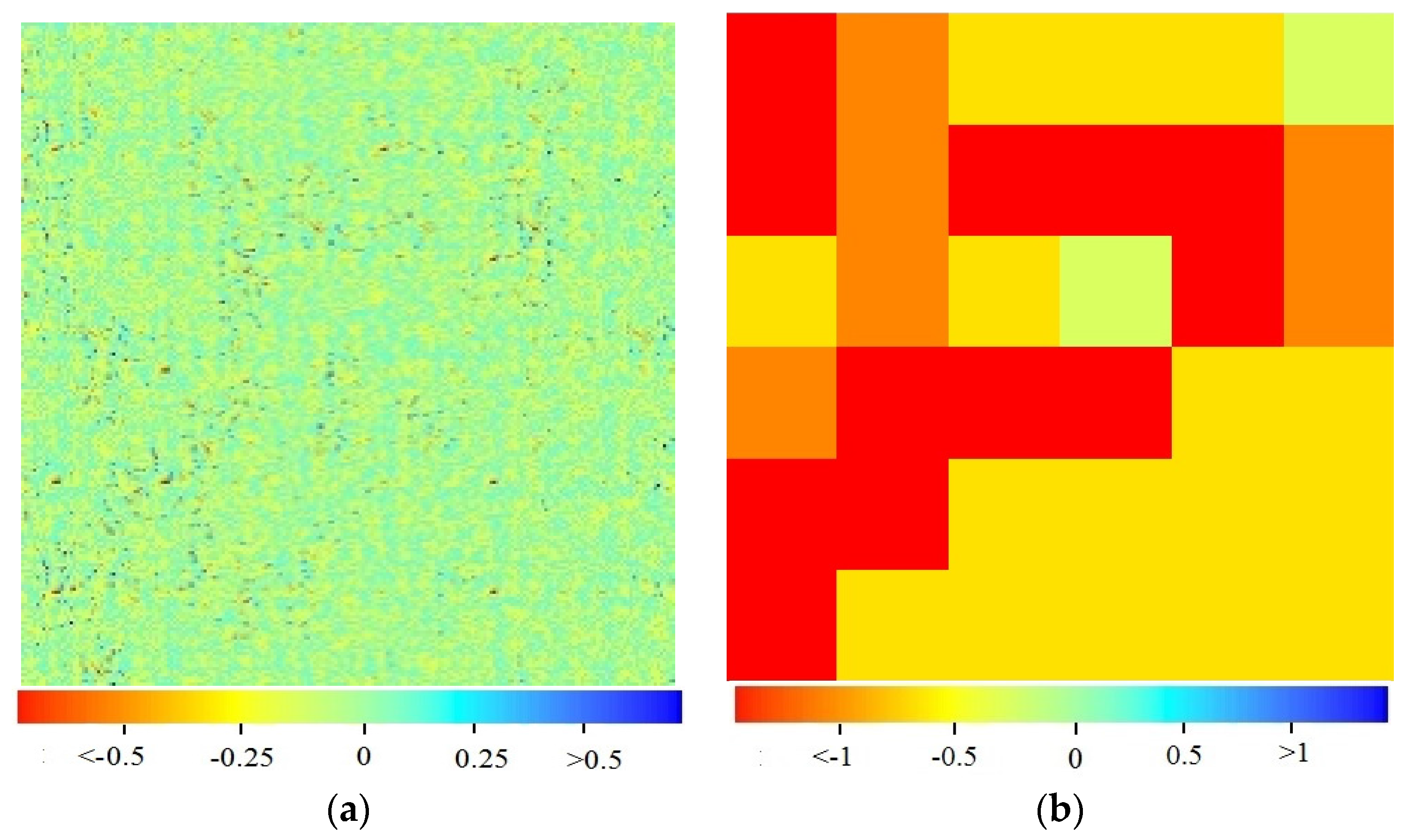
Figure 10a shows the map of differences between the LAI values retrieved from MODIS and TM surface reflectance data and those retrieved only from TM surface reflectance data at the spatial resolution of 28.9 m and Figure 10b shows the map of differences between the LAI values retrieved from MODIS and TM surface reflectance data and those retrieved only from MODIS surface reflectance data of 926.6 m at the Bondville site. Results indicate that the LAI values retrieved only from TM surface reflectance data achieve good agreement with the LAI values retrieved from MODIS and TM surface reflectance data. This is because most details of the LAI values retrieved from the MODIS and TM surface reflectance data are coming from TM surface reflectance data. However, the LAI values retrieved from MODIS and TM surface reflectance data were much larger than those retrieved only from MODIS surface reflectance data (Figure 10b). Figure 9 demonstrates that the LAI values retrieved from MODIS and TM surface reflectance data achieved good agreement with the aggregated LAI reference map values across the whole range of LAI values. In other words, the method in this study can provide improved mapping of LAI at the MODIS resolution by integrating the MODIS and TM/ETM+ surface reflectance data.

For the next step of the study, a dynamical model of LAI that evolves in time will be coupled with the EnMsT. Even though TM/ETM+ reflectance data contains more information compared with MODIS reflectance data on the same day, low time resolution limits its application in the inversion of LAI for time series. If there exist both TM/ETM+ reflectance data and MODIS reflectance data on that day, more details will be got from TM/ETM+ reflectance data. However, if only MODIS reflectance data exists on the day, LAI retrieved from previous time will be used as the input data and MODIS reflectance data will provide more information about changing dynamics of LAI in time series.

In addition, only quad tree is used during the construction of the EnMsT in this study. The EnMsT with 4k number of nodes can make the calculation and formula derivation easier. However, most geographical regions have an arbitrary shape and number of pixels. Thus, in the near future, more complex structure of the EnMsT like neural gas (NG) algorithm [36] will be considered to describe irregular shapes of geographical regions.

5. Conclusions

In this study, a new method was developed to retrieve multiscale LAI values from satellite observations at different spatial resolutions. The average of multi-year MODIS LAI values corresponding to the date of satellite observations was used as a priori knowledge for LAI to construct an initial EnMsT, and a two-sweep filtering procedure was used to update LAI values at each node of the EnMsT by integrating multiple satellite observations with different spatial resolutions. Then, the retrieved LAI values at the finest scale were used as a priori knowledge for LAI for the new round of construction and updating of the EnMsT, until the sum of the difference of LAI values at each node of the EnMsT between two adjacent updates was less than a given threshold.

The method introduced canopy radiative transfer models into the EnMsF to simultaneously retrieve multiscale LAI from MODIS and TM/ETM+ surface reflectance data. Validation of the retrieved LAI at different spatial resolutions against the aggregated LAI reference maps was carried out over several sites with different vegetation types. The results demonstrated that the retrieved LAI values at each spatial resolution were in good agreement with the aggregated LAI reference map values at the corresponding spatial resolution. The retrieved LAI values at the coarsest scale provided better accuracy with the aggregated LAI reference map values compared with the MODIS LAI values.

In this study, the method was only applied to retrieve LAI values by integrating MODIS and TM/ETM+ surface reflectance data at a specific time. In the near future, we will extend the methodology to retrieve multiscale LAI values from time series data obtained by satellite sensors at different spatial resolutions.