
Cropland Mapping over Sahelian and Sudanian Agrosystems: A Knowledge-Based Approach Using PROBA-V Time Series at 100-m


Abstract
:
1. Introduction
2. Materials
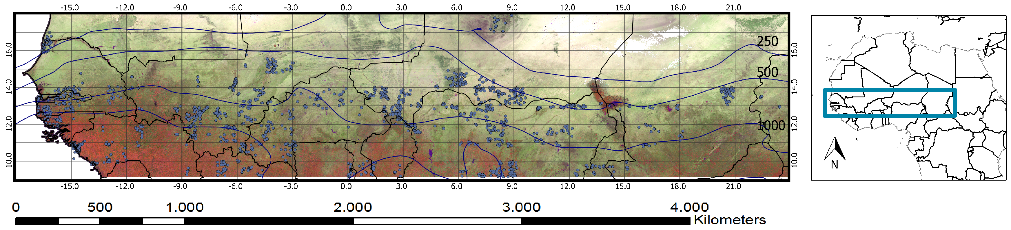
2.1. Study Site
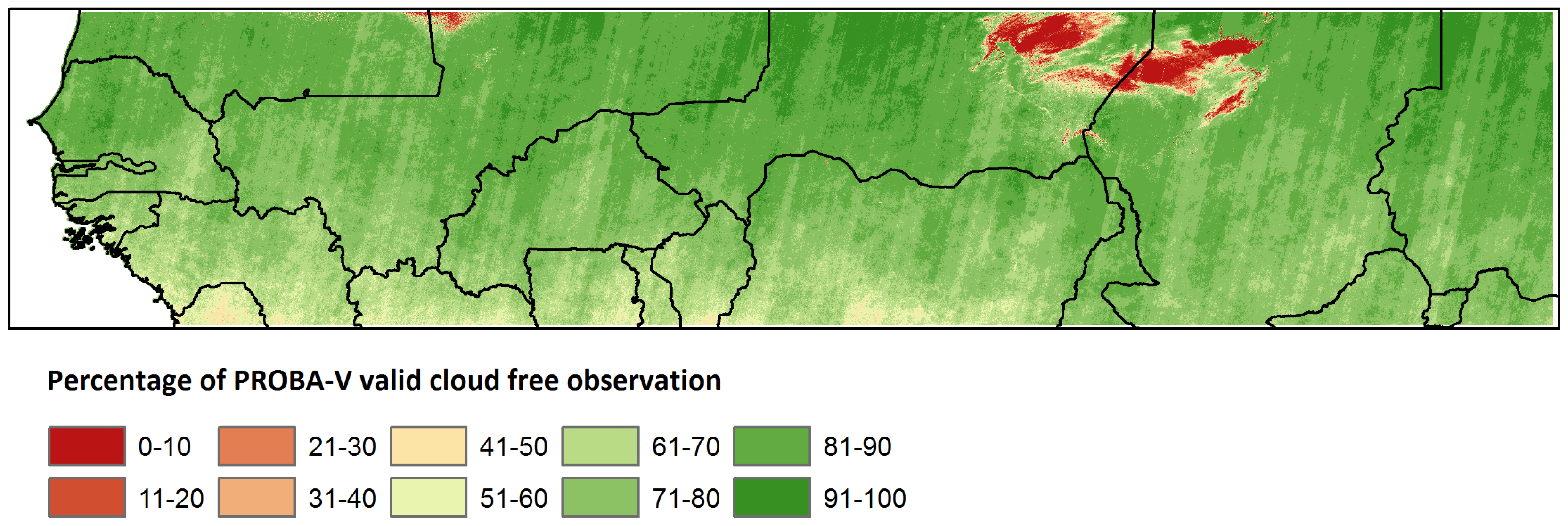
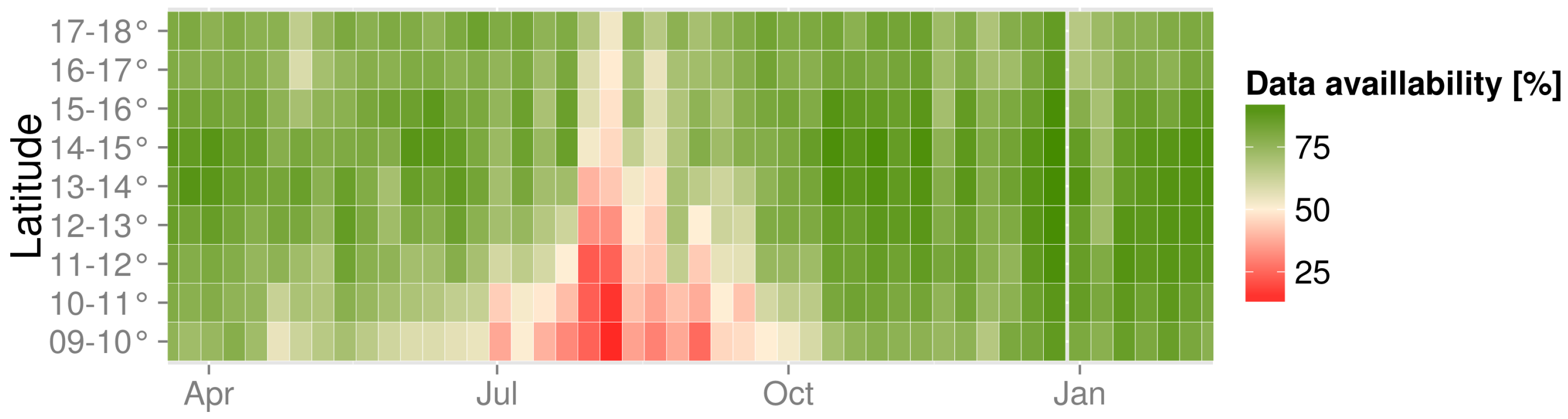
2.2. Data
3. Methodology
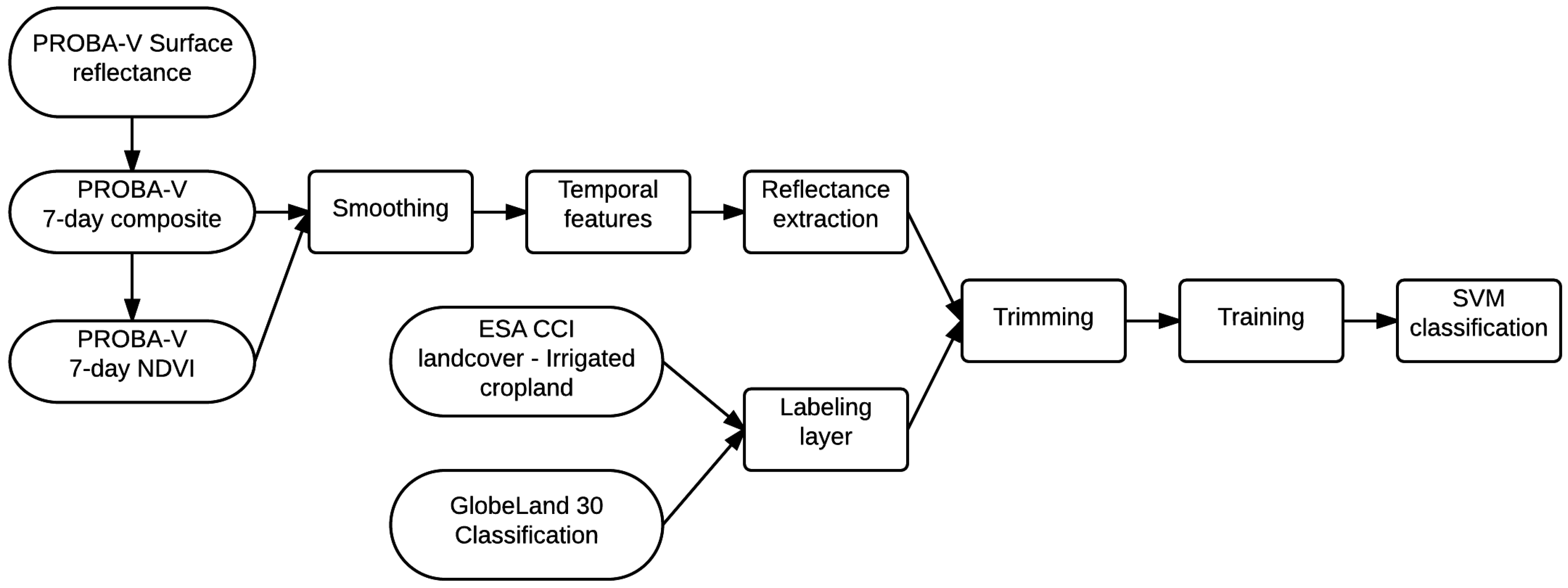
3.1. Cropland Classification
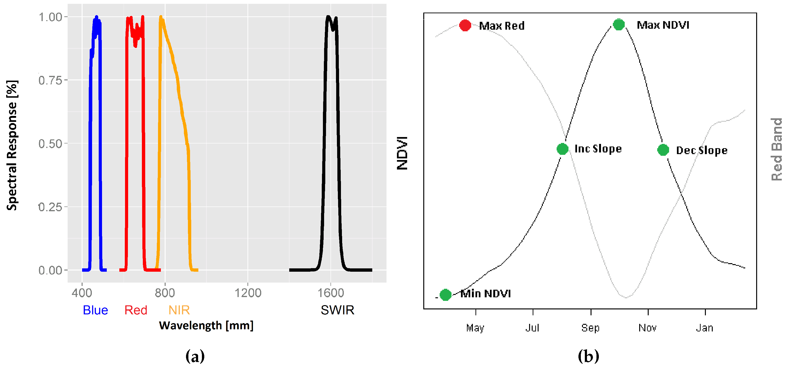
3.1.1. Extracting Temporal Features from PROBA-V
3.1.2. Trimming and Local Training
3.1.3. SVM Classification
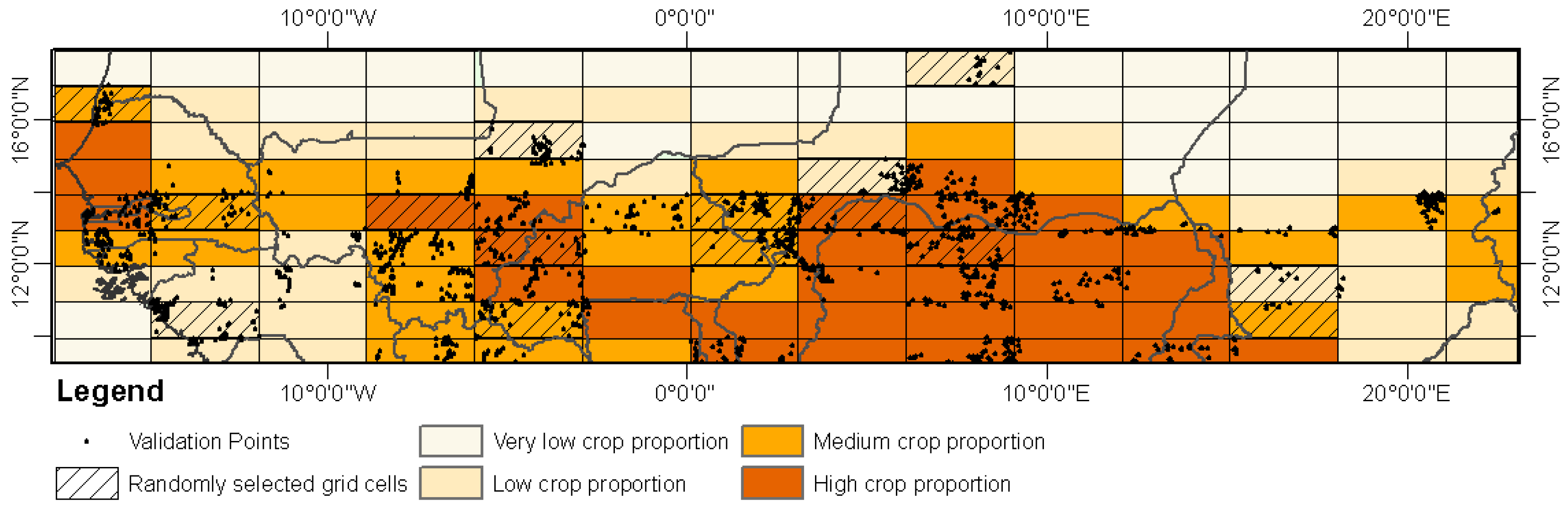
3.2. Handling the Spatial Gradient and the Landscape Diversity
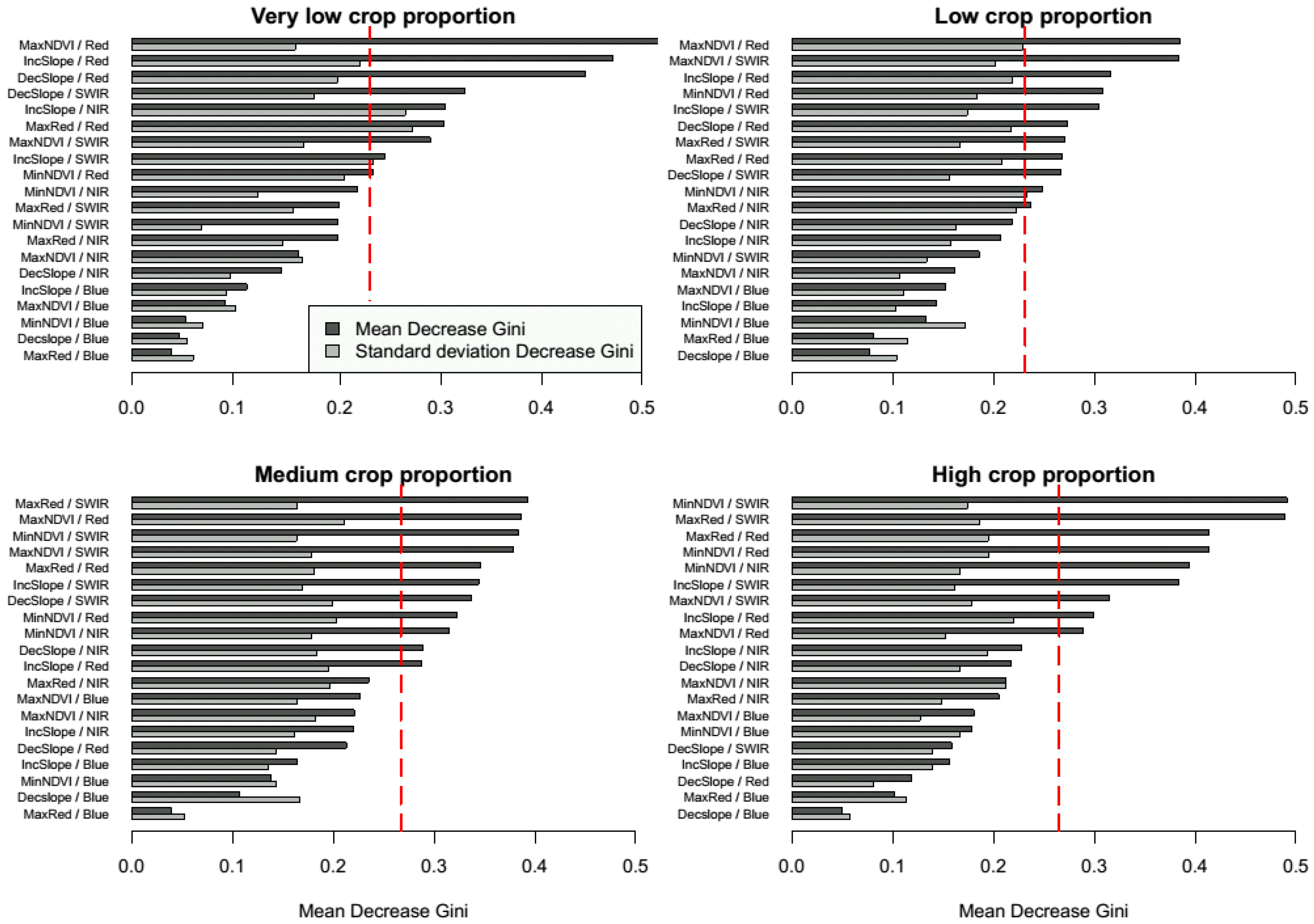
3.3. Relative Importance of Spectral-Temporal Features
3.4. Validation
3.5. Error Analysis
4. Results
4.1. Spectral-Temporal Feature Importance
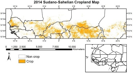
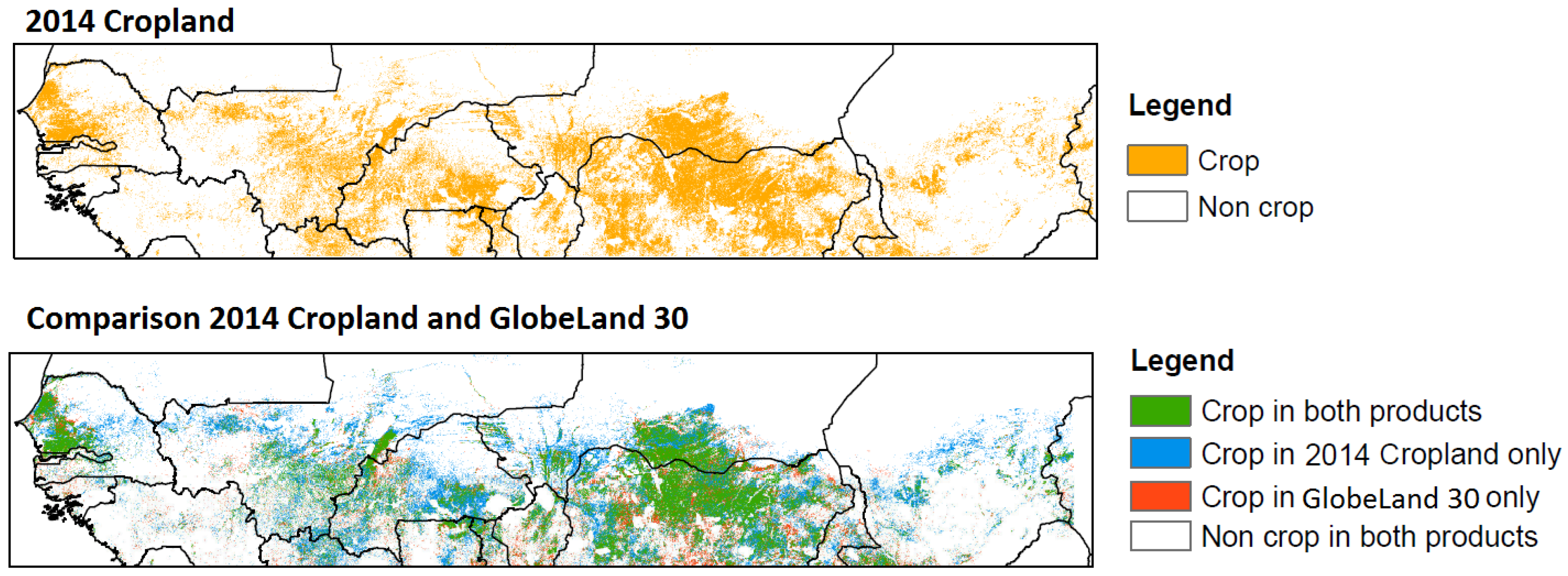
4.2. Qualitative Analysis of 2014 Sudano-Sahelian Cropland map
4.3. Accuracy of the Cropland Map and Comparison with Existing Global Products
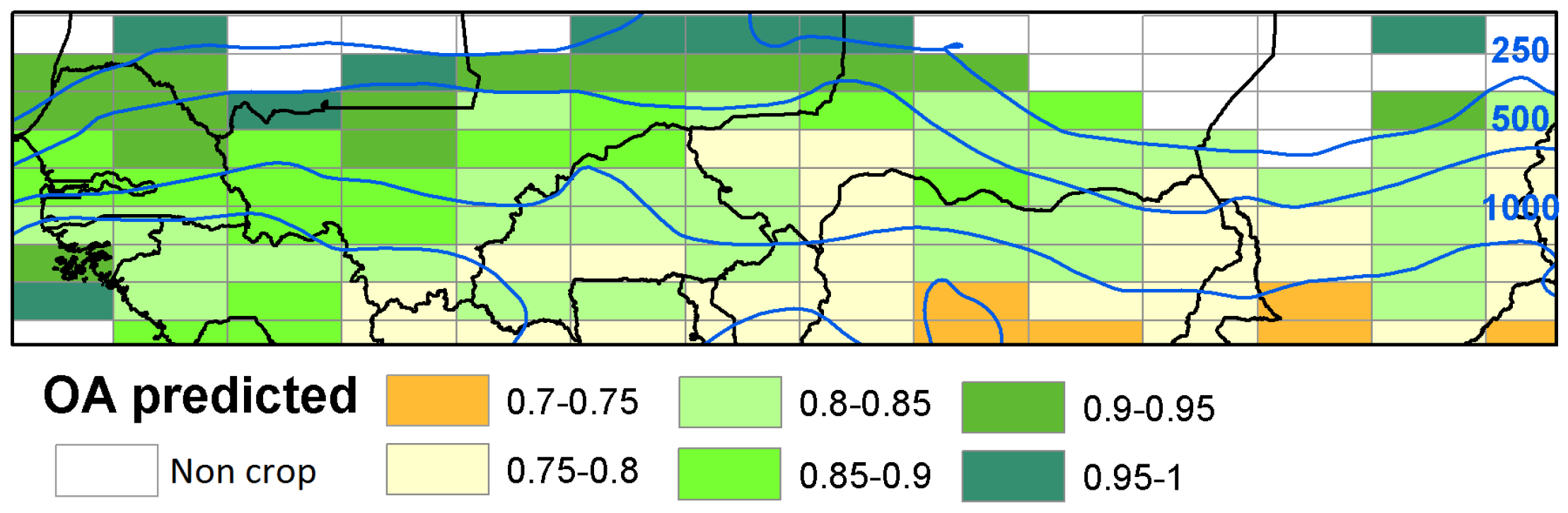
4.4. Spatial Distribution of Errors
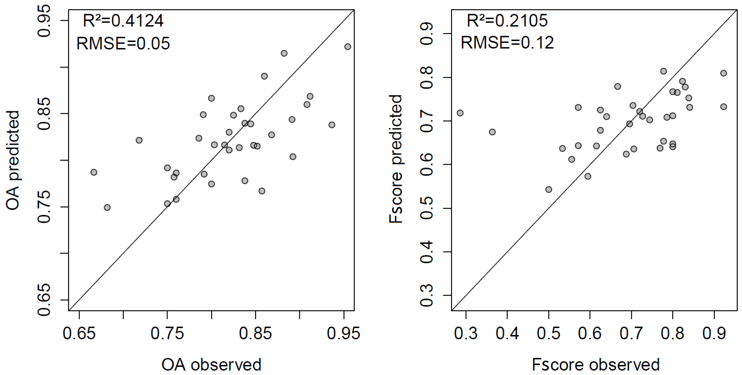
4.5. Multiple Linear Regression to Explain OA and F-Score
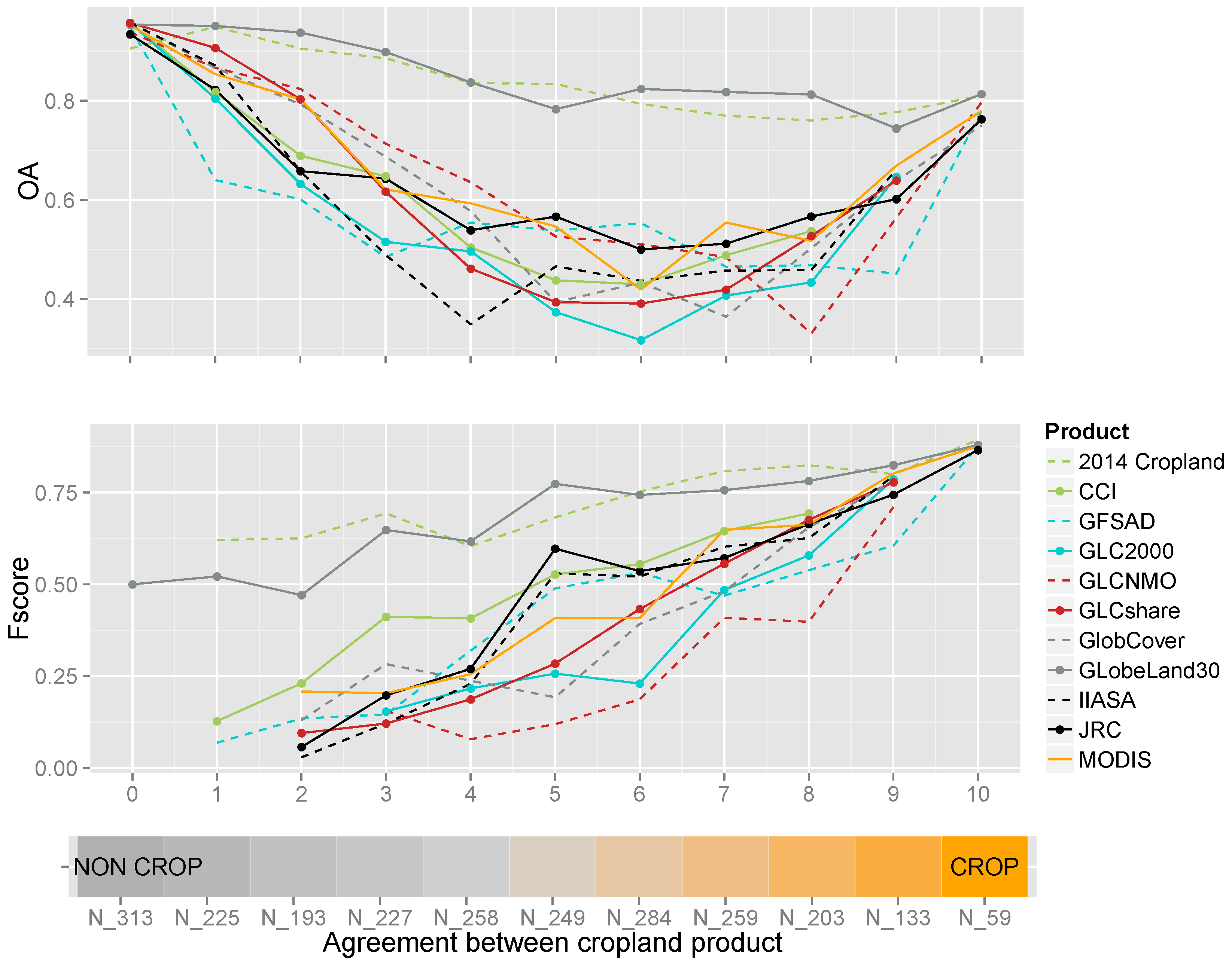
4.6. OA and F-Score in the Disagreement Region of Global Products
4.7. Fragmentation of the Landscape
5. Discussion
6. Conclusions
Acknowledgments
Author Contributions
Conflicts of Interest
References
- CORAF/WECARD. Strategic Plan 2007–2016; CORAF/WECARD: Dakar, Senegal, 2007. [Google Scholar]
- Brevault, T.; Renou, A.; Vayssieres, J.; Amadji, G.; Assogba Komlan, F.; Dalanda Diallo, M.; De Bon, H.; Diarra, K.; Hamadoun, A.; Huat, J.; et al. DIVECOSYS: Bringing together researchers to design ecologically-based pest management for small-scale farming systems in West Africa. Crop Prot. 2014, 66, 53–60. [Google Scholar] [CrossRef]
- Lahmar, R.; Bationo, B.; Dan Lamso, N.; Guero, Y.; Tittonell, P. Tailoring conservation agriculture technologies to West Africa semi-arid zones: Building on traditional local practices for soil restoration. Field Crops Res. 2012, 132, 158–167. [Google Scholar] [CrossRef]
- Jalloh, A.; Roy-Macauley, H.; Sereme, P. Major agro-ecosystems of West and Central Africa: Brief description, species richness, management, environmental limitations and concerns. Agric. Ecosyst. Environ. 2012, 157, 5–16. [Google Scholar] [CrossRef]
- Akponikpe, P.; Minet, J.; Gerard, B.; Defourny, P.; Bielders, C. Spatial fields dispersion as a farmer strategy to reduce agro-climatic risk at the household level in pearl millet-based systems in the Sahel: A modeling perspective. Agric. For. Meteorol. 2011, 151, 215–227. [Google Scholar] [CrossRef]
- Dardel, C.; Kergoat, L.; Hiernaux, P.; Mougin, E.; Grippa, M.; Tucker, C. Re-greening Sahel: 30 years of remote sensing data and field observations (Mali, Niger). Remote Sens. Environ. 2014, 140, 350–364. [Google Scholar] [CrossRef]
- Genesio, L.; Bacci, M.; Baron, C.; Diarra, B.; Di Vecchia, A.; Alhassane, A.; Hassane, I.; Ndiaye, M.; Philippon, N.; Tarchiani, V.; et al. Early warning systems for food security in West Africa: Evolution, achievements and challenges. Atmos. Sci. Lett. 2011, 12, 142–148. [Google Scholar] [CrossRef]
- Karlson, M.; Ostwald, M. Remote sensing of vegetation in the Sudano-Sahelian zone: A literature review from 1975 to 2014. J. Arid Environ. 2015, 124, 257–269. [Google Scholar] [CrossRef]
- Potts, M.; Zulu, E.; Wehner, M.; Castillo, F.; Henderson, C. Crisis in the Sahel: Possible Solutions and the Consequences of Inaction; The OASIS Initiative: Berkeley, CA, USA, 2013. [Google Scholar]
- Bailis, R.; Ezzati, M.; Kammen, D.M. Mortality and greenhouse gas impacts of biomass and petroleum energy futures in Africa. Science 2005, 308, 98–103. [Google Scholar] [CrossRef] [PubMed]
- Manning, A.D.; Gibbons, P.; Lindenmayer, D.B. Scattered trees: A complementary strategy for facilitating adaptive responses to climate change in modified landscapes? J. Appl. Ecol. 2009, 46, 915–919. [Google Scholar] [CrossRef]
- Mertz, O.; D’haen, S.; Maiga, A.; Moussa, I.B.; Barbier, B.; Diouf, A.; Diallo, D.; Da, E.D.; Dabi, D. Climate variability and environmental stress in the Sudan-Sahel zone of West Africa. Ambio 2012, 41, 380–392. [Google Scholar] [CrossRef] [PubMed]
- Liu, J.; Liu, M.; Tian, H.; Zhuang, D.; Zhang, Z.; Zhang, W.; Tang, X.; Deng, X. Spatial and temporal patterns of China s cropland during 1990 2000: An analysis based on Landsat {TM} data. Remote Sens. Environ. 2005, 98, 442–456. [Google Scholar] [CrossRef]
- Delrue, J.; Bydekerke, L.; Eerens, H.; Gilliams, S.; Piccard, I.; Swinnen, E. Crop mapping in countries with small-scale farming: A case study for West Shewa, Ethiopia. Int. J. Remote Sens. 2013, 34, 2566–2582. [Google Scholar] [CrossRef]
- Vancutsem, C.; Marinho, E.; Kayitakire, F.; See, L.; Fritz, S. Harmonizing and combining existing Land Cover/Land Use datasets for cropland area monitoring at the African continental scale. Remote Sens. 2012, 5, 19–41. [Google Scholar] [CrossRef]
- Fritz, S.; See, L.; Rembold, F. Comparison of global and regional land cover maps with statistical information for the agricultural domain in Africa. Int. J. Remote Sens. 2010, 31, 2237–2256. [Google Scholar] [CrossRef]
- Global land cover mapping at 30 m resolution: A POK-based operational approach. ISPRS J. Photogramm. Remote Sens. 2015, 103, 7–27.
- Pittman, K.; Hansen, M.C.; Becker-Reshef, I.; Potapov, P.V.; Justice, C.O. Estimating global cropland extent with multi-year MODIS data. Remote Sens. 2010, 2, 1844–1863. [Google Scholar] [CrossRef]
- Defourny, P. Land Cover CCI: Product user Guide: Version 2; Technical Report; UCL, ESA: Louvain-la-Neuve, Belgium, 2014. [Google Scholar]
- Teluguntla, P.G.; Thenkabail, P.S.; Xiong, J.; Gumma, M.K.; Giri, C.; Milesi, C.; Ozdogan, M.; Congalton, R.; Tilton, J.; Sankey, T.T.; et al. Global Cropland Area Database (GCAD) Derived from Remote Sensing in Support of Food Security in the Twenty-First Century: Current Achievements and Future Possibilities; Taylor & Francis: Boca Raton, FL, USA, 2015; in press. [Google Scholar]
- Bartholomé, E.; Belward, A.S. GLC2000: A new approach to global land cover mapping from Earth observation data. Int. J. Remote Sens. 2005, 26, 1959–1977. [Google Scholar] [CrossRef]
- Ryutaro, T.; Nguyen, T.H.; Toshiyuki, K.; Bayan, A.; Gegen, T.; Dong, X.P. Production of global land cover data GLCNMO2008. J. Geogr. Geol. 2014. [Google Scholar] [CrossRef]
- Bontemps, S.; Defourny, P.; Van Bogaert, E. GLOBCOVER 2009: Product Description and Dalidation Report; Technical Report; UCL, ESA: Louvain-la-Neuve, Belgium, 2011. [Google Scholar]
- Tchuente, A.T.K.; Roujean, J.L.; Faroux, S. ECOCLIMAP-II: An ecosystem classification and land surface parameters database of Western Africa at 1 km resolution for the African Monsoon Multidisciplinary Analysis (AMMA) project. Remote Sens. Environ. 2010, 114, 961–976. [Google Scholar] [CrossRef]
- Latham, J.; Cumani, R.; Rosati, I.; Bloise, M. FAO Global Land Cover (GLC-SHARE) Beta-Release 1.0 Database; FAO: Rome, Italy, 2014. [Google Scholar]
- Biradar, C.; Thenkabail, P.; Noojipady, P.; Li, Y.; Dheeravath, V.; Turral, H.; Velpuri, M.; Gumma, M.; Gangalakunta, O.; Cai, X.; et al. A global map of rainfed cropland areas (GMRCA) at the end of last millennium using remote sensing. Int. J. Appl. Earth Obs. Geoinf. 2009, 11, 114–129. [Google Scholar] [CrossRef]
- Prasad, S.T.; Biradar, C.; Noojipady, P.; Dheeravath, V.; Li, Y.; Velpuri, M.; Gumma, M.; Gangalakunta, O.; Turral, H.; Cai, X.; et al. Global irrigated area map (GIAM), derived from remote sensing, for the end of the last millennium. Int. J. Remote Sens. 2009, 30, 3679–3733. [Google Scholar] [CrossRef]
- Wu, W.; Shibasaki, R.; Yang, P.; Zhou, Q.; Tang, H. Remotely sensed estimation of cropland in China: A comparison of the maps derived from four global land cover datasets. Can. J. Remote Sens. 2008, 34, 467–479. [Google Scholar] [CrossRef]
- Waldner, F.; Fritz, S.; Di Gregorio, A.; Defourny, P. Mapping priorities to focus cropland mapping activities: Fitness assessment of existing global, regional and national cropland maps. Remote Sens. 2015, 7, 7959–7986. [Google Scholar] [CrossRef]
- Fritz, S.; See, L.; You, L.; Justice, C.; Becker-Reshef, I.; Bydekerke, L.; Cumani, R.; Defourny, P.; Erb, K.; Foley, J.; et al. The need for improved maps of global cropland. Eos Trans. Am. Geophys. Union 2013, 94, 31–32. [Google Scholar] [CrossRef]
- Bontemps, S.; Herold, M.; Kooistra, L.; Van Groenestijn, A.; Hartley, A.; Arino, O.; Moreau, I.; Defourny, P. Revisiting land cover observation to address the needs of the climate modeling community. Biogeosciences 2012, 9, 2145–2157. [Google Scholar] [CrossRef]
- Swain, P.; Davis, S. Remote Sensing: The Quantitative Approach; Advanced book program; McGraw-Hill International Book Co.: New York, NY, USA, 1978. [Google Scholar]
- Hansen, M.; Dubayah, R.; Defries, R. Classification trees: An alternative to traditional land cover classifiers. Int. J. Remote Sens. 1996, 17, 1075–1081. [Google Scholar] [CrossRef]
- Lippmann, R. An introduction to computing with neural nets. IEEE ASSP Mag. 1987, 4, 4–22. [Google Scholar] [CrossRef]
- Landgrebe, D. A survey of decision tree classifier methodology. IEEE Trans. Syst. Man Cybern. 1991, 21, 660–674. [Google Scholar]
- Mountrakis, G.; Im, J.; Ogole, C. Support vector machines in remote sensing: A review. ISPRS J. Photogramm. Remote Sens. 2011, 66, 247–259. [Google Scholar] [CrossRef]
- Szuster, B.W.; Chen, Q.; Borger, M. A comparison of classification techniques to support land cover and land use analysis in tropical coastal zones. Appl. Geogr. 2011, 31, 525–532. [Google Scholar] [CrossRef]
- Pal, M.; Mather, P. Assessment of the effectiveness of support vector machines for hyperspectral data. Future Gener. Comput. Syst. 2004, 20, 1215–1225. [Google Scholar] [CrossRef]
- Paneque-Gálvez, J.; Mas, J.F.; Moré, G.; Cristóbal, J.; Orta-Martínez, M.; Luz, A.C.; Guèze, M.; Macía, M.J.; Reyes-García, V. Enhanced land use/cover classification of heterogeneous tropical landscapes using support vector machines and textural homogeneity. Int. J. Appl. Earth Obs. Geoinf. 2013, 23, 372–383. [Google Scholar] [CrossRef]
- Huang, C.; Davis, L.; Townshend, J. An assessment of support vector machines for land cover classification. Int. J. Remote Sens. 2002, 23, 725–749. [Google Scholar] [CrossRef]
- Sivakumar, M. Exploiting rainy season potential from the onset of rains in the Sahelian zone of West Africa. Agric. For. Meteorol. 1990, 51, 321–332. [Google Scholar] [CrossRef]
- Kang, B.T. Moist Savanas of Africa—Potentials and Constraints for Crop Production; ITA: Ibadan, Nigeria, 1995. [Google Scholar]
- Dierckx, W.; Sterckx, S.; Benhadj, I.; Livens, S.; Duhoux, G.; Van Achteren, T.; Francois, M.; Mellab, K.; Saint, G. PROBA-V mission for global vegetation monitoring: Standard products and image quality. Int. J. Remote Sens. 2014, 35, 2589–2614. [Google Scholar] [CrossRef]
- Zhao, Y.; Gong, P.; Yu, L.; Hu, L.; Li, X.; Li, C.; Zhang, H.; Zheng, Y.; Wang, J.; Zhao, Y.; et al. Towards a common validation sample set for global land-cover mapping. Int. J. Remote Sens. 2014, 35, 4795–4814. [Google Scholar] [CrossRef]
- Boschetti, L.; Flasse, S.P.; Brivio, P.A. Analysis of the conflict between omission and commission in low spatial resolution dichotomic thematic products: The Pareto Boundary. Remote Sens. Environ. 2004, 91, 280–292. [Google Scholar] [CrossRef]
- Waldner, F.; Lambert, M.J.; Li, W.; Weiss, M.; Demarez, V.; Morin, D.; Marais-Sicre, C.; Hagolle, O.; Baret, F.; Defourny, P. Land cover and crop type classification along the season based on biophysical variables retrieved from multi-sensor high-resolution time series. Remote Sens. 2015, 7, 10400–10424. [Google Scholar] [CrossRef]
- Matton, N.; Canto, G.S.; Waldner, F.; Valero, S.; Morin, D.; Inglada, J.; Arias, M.; Bontemps, S.; Koetz, B.; Defourny, P. An automated method for annual cropland mapping along the season for various globally-distributed agrosystems using high spatial and temporal resolution time series. Remote Sens. 2015, 7, 13208–13232. [Google Scholar] [CrossRef]
- Waldner, F.; Canto, G.S.; Defourny, P. Automated annual cropland mapping using knowledge-based temporal features. ISPRS J. Photogramm. Remote Sens. 2015, 110, 1–13. [Google Scholar] [CrossRef]
- Akbari, M.; Mamanpoush, A.R.; Gieske, A.; Miranzadeh, M.; Torabi, M.; Salemi, H. Crop and land cover classification in Iran using Landsat 7 imagery. Int. J. Remote Sens. 2006, 27, 4117–4135. [Google Scholar] [CrossRef]
- Eilers, P. A perfect smoother. Anal. Chem. 2003, 75, 3631–3636. [Google Scholar] [CrossRef] [PubMed]
- Atkinson, P.M.; Jeganathan, C.; Dash, J.; Atzberger, C. Inter-comparison of four models for smoothing satellite sensor time-series data to estimate vegetation phenology. Remote Sens. Environ. 2012, 123, 400–417. [Google Scholar] [CrossRef]
- Atzberger, C.; Eilers, P.H. Evaluating the effectiveness of smoothing algorithms in the absence of ground reference measurements. Int. J. Remote Sens. 2011, 32, 3689–3709. [Google Scholar] [CrossRef]
- Foody, G.; Mathur, A. Toward intelligent training of supervised image classifications: Directing training data acquisition for SVM classification. Remote Sens. Environ. 2004, 93, 107–117. [Google Scholar] [CrossRef]
- Wang, L. Support Vector Machines: Theory and Applications; Springer Science & Business Media: Singapore, 2005; Volume 177. [Google Scholar]
- Vapnik, V.N.; Vapnik, V. Statistical Learning Theory; Wiley: New York, NY, USA, 1998; Volume 1. [Google Scholar]
- Hiernaux, P.; Mougin, E.; Diarra, L.; Soumaguel, N.; Lavenu, F.; Tracol, Y.; Diawara, M. Sahelian rangeland response to changes in rainfall over two decades in the Gourma region, Mali. J. Hydrol. 2009, 375, 114–127. [Google Scholar] [CrossRef]
- Bégué, A.; Vintrou, E.; Saad, A.; Hiernaux, P. Differences between cropland and rangeland MODIS phenology (start-of-season) in Mali. Int. J. Appl. Earth Obs. Geoinf. 2014, 31, 167–170. [Google Scholar] [CrossRef]
- Bégué, A.; Vintrou, E.; Ruelland, D.; Claden, M.; Dessay, N. Can a 25-year trend in Soudano-Sahelian vegetation dynamics be interpreted in terms of land use change? A remote sensing approach. Glob. Environ. Chang. 2011, 21, 413–420. [Google Scholar] [CrossRef]
- Renier, C.; Waldner, F.; Jacques, D.C.; Babah Ebbe, M.A.; Cressman, K.; Defourny, P. A dynamic vegetation senescence indicator for near-real-time desert locust habitat monitoring with MODIS. Remote Sens. 2015, 7, 7545–7570. [Google Scholar] [CrossRef]
- Breiman, L. Random forests. Mach. Learn. 2001, 45, 5–32. [Google Scholar] [CrossRef]
- Wagner, J.E.; Stehman, S.V. Optimizing sample size allocation to strata for estimating area and map accuracy. Remote Sens. Environ. 2015, 168, 126–133. [Google Scholar] [CrossRef]
- Foody, G.M. Local characterization of thematic classification accuracy through spatially constrained confusion matrices. Int. J. Remote Sens. 2005, 26, 1217–1228. [Google Scholar] [CrossRef]
- Liu, C.; Frazier, P.; Kumar, L. Comparative assessment of the measures of thematic classification accuracy. Remote Sens. Environ. 2007, 107, 606–616. [Google Scholar] [CrossRef]
- Leroux, L.; Jolivot, A.; Bégué, A.; Seen, D.L.; Zoungrana, B. How reliable is the MODIS land cover product for crop mapping Sub-Saharan agricultural landscapes? Remote Sens. 2014, 6, 8541–8564. [Google Scholar] [CrossRef]
- Foody, G. Status of land cover classification accuracy assessment. Remote Sens. Environ. 2002, 80, 185–201. [Google Scholar] [CrossRef]
- Waldner, F.; Ebbe, M.A.B.; Cressman, K.; Defourny, P. Operational monitoring of the desert locust habitat with earth observation: An assessment. ISPRS Int. J. Geo-Inf. 2015, 4, 2379–2400. [Google Scholar] [CrossRef]
- Turner, M.G.; O’Neill, R.V.; Gardner, R.H.; Milne, B.T. Effects of changing spatial scale on the analysis of landscape pattern. Landsc. Ecol. 1989, 3, 153–162. [Google Scholar] [CrossRef]
- Mayaux, P.; Lambin, E.F. Estimation of tropical forest area from coarse spatial resolution data: A two-step correction function for proportional errors due to spatial aggregation. Remote Sens. Environ. 1995, 53, 1–15. [Google Scholar] [CrossRef]
- Jia, K.; Liang, S.; Wei, X.; Yao, Y.; Su, Y.; Jiang, B.; Wang, X. Land cover classification of Landsat data with phenological features extracted from time series MODIS NDVI data. Remote Sens. 2014, 6, 11518–11532. [Google Scholar] [CrossRef]
- Smith, J.H.; Stehman, S.V.; Wickham, J.D.; Yang, L. Effects of landscape characteristics on land-cover class accuracy. Remote Sens. Environ. 2003, 84, 342–349. [Google Scholar] [CrossRef]
- Latifovic, R.; Olthof, I. Accuracy assessment using sub-pixel fractional error matrices of global land cover products derived from satellite data. Remote Sens. Environ. 2004, 90, 153–165. [Google Scholar] [CrossRef]
- Moody, A.; Woodcock, C.E. The influence of scale and the spatial characteristics of landscapes on land-cover mapping using remote sensing. Landsc. Ecol. 1995, 10, 363–379. [Google Scholar] [CrossRef]
- Roumenina, E.; Atzberger, C.; Vassilev, V.; Dimitrov, P.; Kamenova, I.; Banov, M.; Filchev, L.; Jelev, G. Single-and multi-date crop identification using PROBA-V 100 and 300 m S1 products on Zlatia test site, Bulgaria. Remote Sens. 2015, 7, 13843–13862. [Google Scholar] [CrossRef]
- Sterckx, S.; Benhadj, I.; Duhoux, G.; Livens, S.; Dierckx, W.; Goor, E.; Adriaensen, S.; Heyns, W.; Van Hoof, K.; Strackx, G.; et al. The PROBA-V mission: Image processing and calibration. Int. J. Remote Sens. 2014, 35, 2565–2588. [Google Scholar] [CrossRef]
- Erwin, W.; Wouter, D.; Jan, D.; Else, S. PROBA-V Products User Manual v1.1; VITO: Mol, Belgium, 2014. [Google Scholar]


| Product | Cropland | Product | Cropland |
|---|---|---|---|
| GlobeLand30 | Cultivated land | MODIS | Cropland |
| GFSAD | Cropland, irrigation major | Mosaic cropland/natural vegetation | |
| Cropland, irrigation minor | IIASA | >25% of probability of crop | |
| Cropland, rainfed | CCI | Cropland rainfed | |
| Cropland rainfed minor fragments | Cropland irrigated or post flooding | ||
| Cropland rainfed very minor fragments | Mosaic cropland (>50%)/natural vegetation | ||
| GLCnmo | Cropland: herbaceous crop | Mosaic natural vegetation (>50%) / cropland | |
| Cropland/other vegetation mosaic | GLC2000 | Cultivated and managed areas | |
| Paddy field: graminoid crops/non graminoid crop | Mosaic cropland/shrubland or grass cover | ||
| GlobCover | Rainfed cropland | Mosaic cropland/tree cover/natural vegetation | |
| Mosaic cropland (50%–70%)/vegetation (20%–50%) | JRC MARS | // GlobCover | |
| Mosaic vegetation (50%–70%)/cropland (20%–50%) | |||
| Cultivated and managed areas | |||
| Post-flooding or irrigated croplands | |||
| GLC Share | Cropland |
| Non Crop | Crop | UA [%] | |
|---|---|---|---|
| Non crop | 1431 | 180 | 89 |
| Crop | 185 | 519 | 74 |
| PA [%] | 89 | 74 | OA[%] = 84 |
| OA | F-score | |||
|---|---|---|---|---|
| Correlation | Ranking | Correlation | Ranking | |
| Location | ||||
| Latitude | 0.44 | 2 | 0.33 | 3 |
| Longitude | –0.28 | 5 | –0.09 | 7 |
| Time-series | ||||
| Data availability | 0.25 | 3 | 0.22 | 1 |
| Landscape characteristics | ||||
| Fragmentation | –0.39 | 1 | –0.2 | 6 |
| Entropy | –0.13 | 6 | –0.1 | 8 |
| Matheron Index | –0.29 | 4 | –0.05 | 5 |
| Crop proportion | –0.05 | 8 | 0.09 | 2 |
| Crop fragmentation | –0.24 | 7 | 0.01 | 4 |
| Total variance explained [%] | 41.24 | 21.05 | ||
| Crop Proportion | Very Low | Low | Medium | High |
|---|---|---|---|---|
| Proportion error (30 m–90 m) (%) | NA | −5.2 | −5.2 | −0.6 |
| Proportion error (30 m–300 m) (%) | NA | −29.8 | −27.0 | −5.7 |
© 2016 by the authors; licensee MDPI, Basel, Switzerland. This article is an open access article distributed under the terms and conditions of the Creative Commons by Attribution (CC-BY) license (http://creativecommons.org/licenses/by/4.0/).
Share and Cite
Lambert, M.-J.; Waldner, F.; Defourny, P. Cropland Mapping over Sahelian and Sudanian Agrosystems: A Knowledge-Based Approach Using PROBA-V Time Series at 100-m. Remote Sens. 2016, 8, 232. https://doi.org/10.3390/rs8030232
Lambert M-J, Waldner F, Defourny P. Cropland Mapping over Sahelian and Sudanian Agrosystems: A Knowledge-Based Approach Using PROBA-V Time Series at 100-m. Remote Sensing. 2016; 8(3):232. https://doi.org/10.3390/rs8030232
Chicago/Turabian StyleLambert, Marie-Julie, François Waldner, and Pierre Defourny. 2016. "Cropland Mapping over Sahelian and Sudanian Agrosystems: A Knowledge-Based Approach Using PROBA-V Time Series at 100-m" Remote Sensing 8, no. 3: 232. https://doi.org/10.3390/rs8030232
APA StyleLambert, M.-J., Waldner, F., & Defourny, P. (2016). Cropland Mapping over Sahelian and Sudanian Agrosystems: A Knowledge-Based Approach Using PROBA-V Time Series at 100-m. Remote Sensing, 8(3), 232. https://doi.org/10.3390/rs8030232