
Multiyear Arctic Ice Classification Using ASCAT and SSMIS

Microwave Earth Remote Sensing Laboratory, Brigham Young University, Provo, UT 84602, USA
*
Author to whom correspondence should be addressed.
Remote Sens. 2016, 8(4), 294; https://doi.org/10.3390/rs8040294
Submission received: 5 January 2016
/
Revised: 14 March 2016
/
Accepted: 25 March 2016
/
Published: 30 March 2016
(This article belongs to the Special Issue Sea Ice Remote Sensing and Analysis)
Abstract
:The concentration, type, and extent of sea ice in the Arctic can be estimated based on measurements from satellite active microwave sensors, passive microwave sensors, or both. Here, data from the Advanced Scatterometer (ASCAT) and the Special Sensor Microwave Imager/Sounder (SSMIS) are employed to broadly classify Arctic sea ice type as first-year (FY) or multiyear (MY). Combining data from both active and passive sensors can improve the performance of MY and FY ice classification. The classification method uses C-band measurements from ASCAT and 37 GHz brightness temperature measurements from SSMIS to derive a probabilistic model based on a multivariate Gaussian distribution. Using a Gaussian model, a Bayesian estimator selects between FY and MY ice to classify pixels in images of Arctic sea ice. The ASCAT/SSMIS classification results are compared with classifications using the Oceansat-2 scatterometer (OSCAT), the Equal-Area Scalable Earth Grid (EASE-Grid) Sea Ice Age dataset available from the National Snow and Ice Data Center (NSIDC), and the Canadian Ice Service (CIS) charts, also available from the NSIDC. The MY ice extent of the ASCAT/SSMIS classifications demonstrates an average difference of 282 thousand km from that of the OSCAT classifications from 2009 to 2014. The difference is an average of 13.6% of the OSCAT MY ice extent, which averaged 2.19 million km over the same period. Compared to the ice classified as two years or older in the EASE-Grid Sea Ice Age dataset (EASE-2+) from 2009 to 2012, the average difference is 617 thousand km. The difference is an average of 22.8% of the EASE-2+ MY ice extent, which averaged 2.79 million km from 2009 to 2012. Comparison with the Canadian Ice Service (CIS) charts shows that most ASCAT/SSMIS classifications of MY ice correspond to a MY ice concentration of approximately 50% or greater in the CIS charts. The addition of the passive SSMIS data appears to improve classifications by mitigating misclassifications caused by ASCAT's sensitivity to rough patches of ice which can appear similar to, but are not, MY ice.

1. Introduction
The physical properties of Arctic sea ice evolve with each year of age, resulting in differences in porosity, salinity, and roughness between first-year (FY) and multiyear (MY) sea ice. Such physical differences produce a difference in the microwave signatures from FY and MY sea ice and enable classification of sea ice type in the Arctic using microwave sensors.
Various algorithms have been devised for classification of sea ice type using active sensors, passive sensors, or both. Scatterometer classification of FY and MY ice has been accomplished using a threshold on the radar backscatter coefficient () [1,2,3], and techniques for ice classification using synthetic aperture radar (SAR) have been explored and developed [4,5,6,7]. SAR has also been employed to evaluate scatterometer classifications [3]. Passive microwave sensors have been used to classify areas of MY ice [8,9,10,11,12] in addition to estimating the extent and concentration of sea ice [12,13]. In addition, fusion of both active and passive microwave sensor data has been employed to classify ice type. Techniques for ice classification using a combination of QuikSCAT and AMSR-E data are described by Shokr and Agnew [14] and Yu et al. [15], while Walker et al. [16] describe a method for ice classification using QuikSCAT combined with NASA Team ice concentration data.
Efforts to develop effective techniques for remote sensing of sea ice are partly motivated by the importance of sea ice and its effects on global climate and ocean dynamics. The insulating layer of sea ice strongly reduces ocean-atmosphere heat exchange during the freezing season, and the high albedo of sea ice also helps to regulate climate by reflecting electromagnetic energy from the sun back into space. The decline of sea ice area can impact atmospheric circulation [17], leading to changing weather patterns [18]. Changes in sea ice cover can also lead to changes in ocean current patterns [19].
Large changes to MY ice coverage over the Arctic within recent decades also motivate the continued monitoring of the composition and extent of Arctic sea ice. Within the past decades, coverage of MY ice has declined [11] and Arctic ice has become younger overall [20]. As MY ice tends to be thicker than FY ice, it is suggested that the total sea ice volume has decreased [21]. Ice type classifications can contribute to studies of Arctic ice volume, having application in altimetry-based ice thickness modeling [22].
Previous ice type classification records have been developed using the SeaWinds scatterometer instrument on the QuikSCAT satellite and the scatterometer onboard the Indian Space Research Organization Oceansat-2 (OSCAT) [1,2,3], though as of 2009 and 2014, respectively, these sensors are no longer fully operational. Extending the scatterometer classification data record beyond 2014 requires use of another sensor. Lack of a currently operational polar-orbiting Ku-band active sensor with readily available data motivates the use of the C-band Advanced Scatterometer (ASCAT), which was launched in 2006 aboard the MetOp-A platform by the European Organisation for the Exploitation of Meteorological Satellites (EUMETSAT) and continues to operate [23,24,25].
In general, the lower frequency of the ASCAT sensor at 40 degrees incidence angle (V-polarized) compared to OSCAT or QuikSCAT at 57.6 and 54 degrees incidence angle (V-polarized) results in measurements that are less sensitive to differences between FY and MY ice. At Ku-band wavelengths (2.24 cm for QuikSCAT/OSCAT), volume scattering from air pockets in porous MY ice results in higher values than from FY ice. At C-band, such air pockets are small relative to the wavelength (5.7 cm for ASCAT) and so lower values are observed [26]. FY ice exhibits lower values relative to MY ice in part because of a higher brine content which increases electromagnetic absorption and reduces backscatter [27]. Hence the separation between FY and MY ice is typically smaller at C-band than at Ku-band. Ice classification at C-band is also complicated by high sensitivity, relative to Ku-band, to rough surface features: backscatter from rough, fractured ice near the ice edge can appear similar to backscatter from MY ice [23]. Though the incidence angles between the sensors differ, the slope of the sea ice backscatter response versus incidence angle at Ku-band is similar to the slope at C-band across the range of incidence angles from 40 to 60 degrees [26], so the effect of the difference in incidence angle is small relative to the effect of the difference in frequency.
In an attempt to compensate for decreased sensitivity at C-band and to increase the information available to the classification algorithm, we exploit data from the 37 GHz channel of the Special Sensor Microwave Imager/Sounder (SSMIS) to aid in distinguishing distributions of FY and MY ice. SSMIS is a passive microwave radiometer first launched aboard the Defense Meteorological Satellite Program (DMSP) F-16 satellite in 2003. The sensor is currently operational aboard the DMSP F-16, F-17, and F-18 satellites.
SSMIS measures the brightness temperature, or intensity of the microwave energy emitted by the earth. During the winter season, FY and MY Arctic sea ice can be discriminated by brightness temperature because of their differing emissivities [11]. The high salinity content of FY ice relative to MY ice results in increased absorption of electromagnetic energy in FY ice and susceptibility to scattering in MY ice [11]. The scattering of electromagnetic energy by air pockets in porous MY ice leads to low emissivity, while FY is typified by high emissivity [28,29].
2. Methodology
The winter season backscatter properties of sea ice at Ku-band result in a bimodal distribution of measurements over the Arctic with the distribution modes representing FY and MY ice occurring between approximately −25 and −18 dB and −12 and −10 dB, respectively [1]. To illustrate the separation of FY and MY ice at Ku-band and C-band, time series of daily histograms from resolution enhanced QuikSCAT and ASCAT data at 40 degrees incidence angle are shown in Figure 1. The data are obtained from the Scatterometer Climate Record Pathfinder [30]. Histograms of are produced for each day and concatenated together to create the time series. Only Arctic values from within the sea ice extent are used, where the extent is identified by a 40% threshold on a daily NASA Team sea ice concentration product [31]. Data are shown for the winters of 2000/2001 and 2001/2002 for QuikSCAT and 2010/2011 and 2011/2012 for ASCAT.
In the figure, the backscatter distributions are shown from day of year 287 to 141 of the next year. Classifications of sea ice are completed for days 284 to 134 of the next year; they are not completed during the summer melt because the backscatter signatures of FY and MY ice become similar, resulting in poor ice classification results. In the QuikSCAT histograms, regions of high bin count for greater than −12 dB and less than −17 dB can be identified and correspond to distributions of MY and FY ice, respectively [1,2].
The QuikSCAT and OSCAT ice classifications [2] use a threshold fitted to a minimum histogram bin count between FY and MY ice distributions in a time series of histograms (as in Figure 1) to classify ice as FY or MY. In this classification scheme, pixels with measurements above the threshold are classified as MY ice, and those with measurements below the threshold are classified as FY ice. While a region of minimum bin count between the two modes can be easily observed in the QuikSCAT histograms, in the ASCAT histograms, two separate regions of high bin count which can be associated with FY and MY ice cannot be identified. As distributions of MY and FY ice are not as separated in the ASCAT histograms as in the QuikSCAT histograms, the thresholding method used by Swan and Long [1] and Lindell and Long [2] to classify FY and MY ice may not be as effective for ASCAT as it was for the Ku-band sensors, QuikSCAT and OSCAT. Rather than continuing the QuikSCAT/OSCAT ice classification record with ASCAT using the same classification methodology as [2], we show how a Bayesian classification algorithm, which uses data from ASCAT and SSMIS, can be used to classify ice type.
2.1. Sensor Information
A summary of the characteristics of the ASCAT and SSMIS sensors is shown in Table 1. The ASCAT sensor is a fan beam scatterometer launched in 2006 into a sun-synchronous near-polar orbit. It operates at 5.255 GHz (C-band) and continues to deliver near-global daily coverage. The SSMIS sensor is a passive microwave radiometer and was launched aboard the Defense Meteorological Satellite Program (DMSP) F-16, F-17, and F-18 platforms in 2003, 2006, and 2009. SSMIS operates at 24 different frequency channels and can collect atmospheric temperature measurements and brightness temperature measurements at a number of different polarizations and frequencies. In this study, data from SSMIS aboard the F-17 platform are used because it provides measurements for the full period of the ASCAT mission.
2.2. Sensors and Data Sources
The new classification method is completed using data from ASCAT and from the 37 GHz V-polarization (V) channel of SSMIS. The choice of frequency channel is motivated by the sensitivity to differences between FY and MY ice. While the 19 GHz V and 19 GHz H-polarization (H) channels are also available, the brightness temperature separation between FY and MY ice at these channels is not as great as the 37 GHz channel. In the NASA Team algorithm [12], brightness temperature measurements for known areas of 100% FY and MY ice are referred to as ice “tie-points” and are shown in Table 2 [12].The table shows that the brightness temperatures of FY and MY ice are separated by approximately 66.5 K for 37 GHz V, 38.9 K for 19 GHz H, and by 35 K for 19 GHz V.
SSMIS data are obtained from the National Snow and Ice Data Center (NSIDC) [34], which provides daily average Arctic brightness temperature images on a 25 km/pixel resolution grid in a polar stereographic projection. To improve the detection of high-resolution features in the FY and MY ice classifications, we incorporate the enhanced resolution ASCAT data [30] and interpolate the SSMIS data onto the ASCAT 4.45 km/pixel grid in the polar stereographic projection. Though a technique for resolution enhancement of radiometer data [35] has been applied to data from the Special Sensor Imager (SSM/I) and the Advanced Microwave Scanning Radiometer-Earth Observing System (AMSR-E), the resulting datasets do not contain data for years after 2011 [30]. We therefore choose to combine the nominal resolution SSMIS data, which are available for the extent of the ASCAT dataset, with the resolution-enhanced ASCAT data.
ASCAT enhanced-resolution data are obtained from the Scatterometer Climate Record Pathfinder [30], which provides daily postings of two-day averaged ASCAT Arctic data normalized to 40 degrees incidence angle and gridded at 4.45 km/pixel resolution in a polar stereographic projection. The enhanced resolution data are produced using the Scatterometer Image Reconstruction (SIR) algorithm [36], a modified algebraic image reconstruction technique which employs the sampling geometry and spatial response function (SRF) of the ASCAT sensor [37]. The SRF describes the contribution of each area within the antenna footprint to the measured value of . Each ASCAT measurement represents an integration of weighted by the spatial response function over the area illuminated by the antenna. For a fine pixel grid, the area illuminated by the antenna encompasses multiple pixels, so if the SRF is known for a given measurement, information about multiple pixel values can be inferred from the single measurement. The SIR algorithm exploits knowledge of the ASCAT spatial response function to reconstruct onto a fine pixel grid.
The two-day averaged reconstructed ASCAT data provide full coverage of the Arctic. As multiple passes of data are required, it is assumed that the backscatter does not change substantially over the time the measurements are taken.
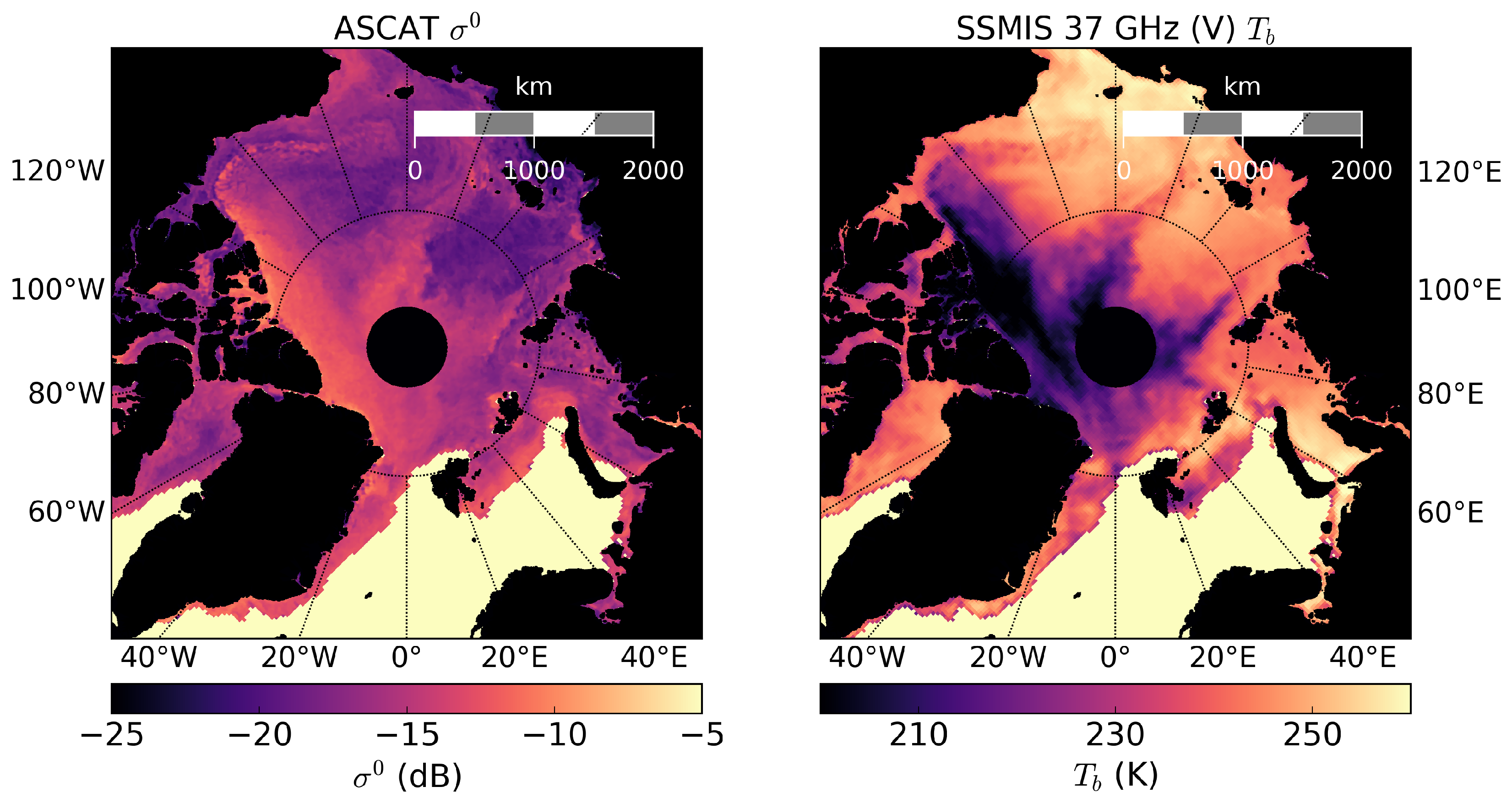
Example Arctic sea ice data from ASCAT and SSMIS for arbitrarily selected day of year 61, 2011 are shown in Figure 2. The main areas of MY ice can be visually identified by locating areas containing higher values and lower brightness temperatures compared to the rest of the ice extent.
Following the QuikSCAT/OSCAT classification scheme [2], the area of classification is restricted to within the ice extent by applying a 40% threshold to a daily NASA Team ice concentration product [31]. The NASA Team product was selected because of its consistent performance [38] and the long time series of available data, which continue to be published. Data from pixels in the ASCAT and SSMIS 37 GHz products which fall within the 40% ice extent are collocated and classified as FY or MY ice. Ice types are classified using a Bayesian estimator where the likelihood and a priori probabilities are initialized at the beginning of winter using the ASCAT/SSMIS classifications from the previous winter and then updated iteratively as subsequent classifications are processed.
2.3. Comparison Datasets
The classification results are compared to classifications of MY and FY ice using OSCAT [2] and to classifications from two other datasets: the EASE-Grid Sea Ice Age dataset [39], and the Canadian Ice Service (CIS) Arctic Regional Sea Ice Charts [40]. Both datasets are provided by the NSIDC.
The EASE-Grid Sea Ice Age dataset is produced from 1979 onward and reports the age of sea ice in years on a 12.5 km/pixel Equal-Area Scalable Earth (EASE) grid. The ice age estimates are produced using sea ice motion vectors derived from a Lagrangian tracking procedure [41,42]. The trajectories of grid cells containing ice are estimated over the years, and the age of tracked ice is recorded. For comparison with the ASCAT/SSMIS classifications, the extent of MY ice in the EASE-Grid Sea Ice Age dataset is calculated by interpolating the ice age data onto the ASCAT/SSMIS grid and summing the area of the grid cells with ice age labels of two years or greater.
An analysis of tracking error has been completed by Kwok et al., who use motion vectors derived from SSM/I data to track ice parcels and compare the estimated trajectories to buoy motion trajectories and trajectories derived from SAR data [43]. Though the dataset for which Kwok et al. complete their analysis is independent from the EASE-Grid Sea Ice Age dataset, the results of the analysis are instructive. They find the location error to be approximately 5 to 12 km per day; the errors do not necessarily accumulate, as annual location error is on the order of 50–100 km [43]. In the EASE-Grid product, similar tracking errors may exist, and the extent of older ice may be overrepresented because each grid cell classification describes the oldest type of ice present and not necessarily the most abundant type of ice [42]. We use the EASE-Grid Sea Ice Age product with the ASCAT/SSMIS classifications to compare the total extent of pixels classified as MY or FY ice. As the comparison deals with extent rather than location, it should be relatively insensitive to the errors in ice location tracking.
The CIS charts are prepared by the Canadian Ice Service and are typically available at weekly intervals from the year 2006 onward [40]. Each ice chart is prepared manually from inspection of in situ observations and from satellite data [44]. Charts are prepared with data from up to 72 hours prior to the reported date.
Ice charts are produced for different regions of the Canadian Arctic, including the Western Arctic, Eastern Arctic, the Hudson bay, the Great Lakes, and the East Coast. As the Western Arctic region has the most overlap with the ASCAT/SSMIS classifications, it is selected for comparison.
Various characteristics of ice are reported in the charts, including the total ice concentration, ice form, and stage of development. In each region, the charts outline subregions of approximately homogeneous ice properties. Total ice concentration is reported, as well as properties of the three thickest ice types: the partial ice concentration, the stage of development or thickness, and the ice form or floe size. The sum of the three reported partial ice concentrations is always less than or equal to the reported total ice concentration.
To compare the ASCAT/SSMIS classifications to the CIS charts, we identify areas of total ice concentration greater than 40% in the CIS charts and follow the procedure of Swan and Long [1]. All ice stages having survived at least one melt season in the CIS charts (second-year ice, MY ice, and old ice) are grouped as MY ice, while all other ice types are grouped as FY ice. For each subregion detailed in a given CIS chart, the three ice types are identified as FY or MY ice and their concentrations are summed to determine a FY and MY ice concentration. The CIS chart subregions are defined by polygons (using latitude and longitude points), so we collocate the CIS chart data with the ASCAT/SSMIS classifications by identifying pixels on the ASCAT/SSMIS grid which fall within each polygon. The ASCAT/SSMIS classifications can then be compared to the CIS chart subregions, and the MY and FY ice concentrations are observed for which ice is typically classified as FY or MY using ASCAT/SSMIS.
2.4. ASCAT/SSMIS Classification
The classification of FY and MY ice with ASCAT and SSMIS uses a Bayesian decision model. The classification is completed by iterating over all pixels within the ice extent and using the decision model to select FY or MY ice. The input to the decision function is a measurement column vector, , which is given as
where consists of an ASCAT measurement and an SSMIS 37 GHz brightness temperature measurement of the same pixel; the SSMIS data are from the first of the two days corresponding to the ASCAT measurement.
The Bayesian classification decides whether the probability of FY ice () given the measurement vector is greater than the probability of MY ice () given , or
Using Bayes’ rule, an equivalent decision is derived in terms of the FY and MY ice distributions: the probabilities of with the assumption that is an observation of FY or MY ice, or
which can be practically implemented.
The multivariate normal expression used for the probabilistic model is given as
where is the data covariance matrix, is the determinant of , and μ is the mean vector. The probabilities and are determined by evaluating where and μ are estimated for FY and MY ice from and brightness temperature measurements of FY and MY ice.
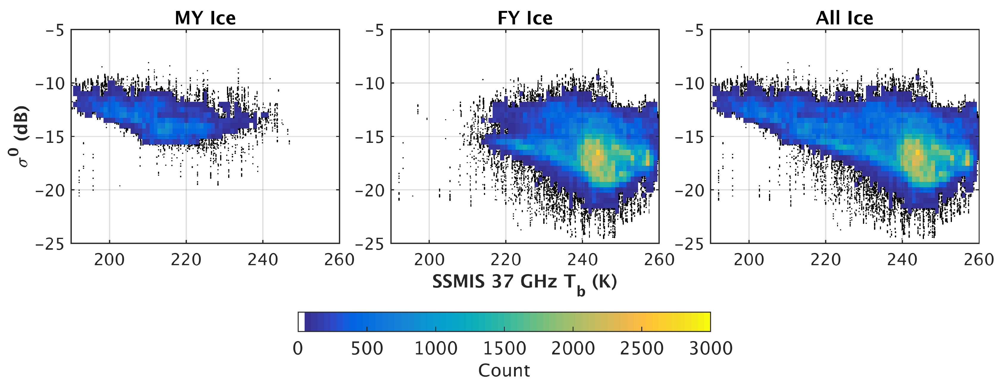
The distributions of FY and MY ice can be observed by visually inspecting scatterplots of brightness temperature and values from the sensors. Joint scatterplots/2D histograms are shown in Figure 3 for data from day of year 61, 2011. The joint scatterplots/2D histograms plot ASCAT versus SSMIS 37 GHz data points. In areas where the scatterplot point density is too great to be able to discern individual points, a 2D histogram is used. The distributions of FY and MY ice are also plotted, using the OSCAT ice type classifications to identify pixels corresponding to FY or MY ice [2]. The plots show that distributions of FY and MY ice are moderately separated, motivating the use of the Bayesian decision model for classification.
The first ice classifications are processed for day of year 284, 2009 using the QuikSCAT classifications [2] to identify the areas of FY and MY ice in the ASCAT and SSMIS data. Areas of FY and MY ice are identified for days 284 to 289, 2009, and the mean and covariance values of the brightness temperature and measurements from regions occupied by FY and MY ice are used to calculate and and initialize the processing. The probabilities of FY and MY ice ( and ) are also calculated from these data by calculating number of pixels classified as FY or MY ice divided by the total number of pixels within the ice extent.
Using the calculated mean, covariance values, and probability values, the first classification of grid cells as FY and MY ice is carried out for day of year 284, 2009 using the ASCAT/SSMIS data. Completed classifications are used to recalculate the mean, covariance, and probability values for FY and MY ice, and an average of the calculated statistics for the five previously classified days are used for successive classifications. After the first five classifications are completed, the statistics used to initialize classifications for day of year 284 are no longer used. At that point, classifications rely on the statistics generated from the classifications for days after day 284. This initial procedure is repeated for every year after 2009. Instead of using OSCAT results for the initialization, however, ASCAT/SSMIS data and classifications from the previous year are used to initialize the statistics and probabilities. As ice is not classified during the summer melt, and classifications begin on day of year 284, we choose to use the prior year’s statistical and probabilistic data, or a priori data, to re-initialize the processing.
Some days in the ASCAT and SSMIS datasets have gaps or are missing data. Data from these days are not used to update the a priori data used for classification. Instead, subsequent classifications rely on the a priori data from the five previously completed classifications where no data was missing.
In the marginal ice zone (MIZ), the area at the interface between sea ice and open water, ocean dynamics can result in rough, broken patches of sea ice, leading to areas of increased backscatter near the sea ice edge. Areas of MY ice are typically characterized by greater backscatter levels than FY ice, and such high backscatter levels from ocean regions near the ice edge can result in erroneous MY ice classification. The ASCAT sensor is sensitive to such areas of rough or broken ice, and so using data from the ASCAT sensor alone to complete the classifications becomes impractical as the Bayesian parameters quickly become corrupted by ice misclassifications, leading to more and more errors. Addition of the SSMIS data mitigates the amount of misclassified ice and provides more information for the Bayesian estimator; however, some areas of misclassified ice remain near the ice edge. To further reduce such areas of misclassified ice, we employ a two-step correction procedure. We embed the first step of the correction procedure in the Bayesian approach by introducing cost functions. In the second step, after the initial classifications are completed, we employ the MIZ correction algorithm described in [2]. The MIZ correction algorithm identifies main areas of MY ice which are consistent from day to day and reclassifies transient areas of MY ice outside the main area of MY ice to FY ice.
To mitigate the apparent misclassifications, cost functions, and , are introduced to the Bayesian decision model and updated for each day of classification. The main areas of MY ice are identified by selecting all grid cells which fall into an area given by the boundary between FY and MY ice contracted by approximately 65 km (15 grid cell lengths) away from the FY ice region. Similarly, main areas of FY ice are identified by selecting all grid cells which fall into an area given by the same boundary but contracted by 65 km away from the MY ice region. The 65 km distance on each side of the FY/MY ice boundary is assumed to adequately allow for possible movement of areas of FY and MY ice from day to day. For the initial classification (before boundaries of FY and MY ice are known), the cost functions are set to a value of one and have no effect on the classifications.
After the initial classification, the cost function is set to a high value (near unity) for pixels within the main area of MY ice, as identified by the contraction operation described previously. For areas within the main area of FY ice, is set to a low value (near zero). The cost function is set in a similar fashion for pixels within and without main areas of FY ice. For areas near the FY/MY boundary, the cost functions take on a value of one, and so have no effect. The cost functions are binary, and so only take on one of the two values for a given pixel. With the addition of the cost functions, the Bayesian decision model becomes
and this model is used for ice classification.
As an experiment, the Bayesian algorithm is also used to process classifications using ASCAT data only and SSMIS 37 GHz data only. For these classifications, we use the same procedure as for ASCAT/SSMIS, except that Equation (1) is modified to contain the appropriate measurements, and the normal probability density function (Equation (4)) is changed to the univariate case. For the ASCAT-only classifications, we incorporate the corrections for MIZ misclassifications. Such misclassifications do not appear in the SSMIS-only classifications, so we incorporate neither the cost functions nor the MIZ correction algorithm. While the SSMIS classifications are comparable to the ASCAT/SSMIS classifications, using the Bayesian estimator with ASCAT-only data produces untenable results. For the ASCAT-only case, misclassifications appear despite the cost functions and corrupt the a priori probabilities, leading to increasing error in the classifications.
3. Results and Discussion
The decision model is applied to data for the years 2009 to 2014 to create classification images for each day. The ASCAT/SSMIS classifications are compared to the OSCAT classifications [2], the CIS charts [40], and the EASE-Grid Sea Ice Age dataset [39]. The CIS charts are used to find the typical concentration of MY ice for which an area of ice is classified as MY using ASCAT/SSMIS. A time series analysis of annual minimum total ice extent and MY ice extent is also completed using extent data from the ASCAT/SSMIS classifications, OSCAT classifications, and the EASE-Grid Sea Ice Age dataset [39]. Extent data are also included for classifications processed using the same methodology as the ASCAT/SSMIS classifications, but only using SSMIS data for comparison.
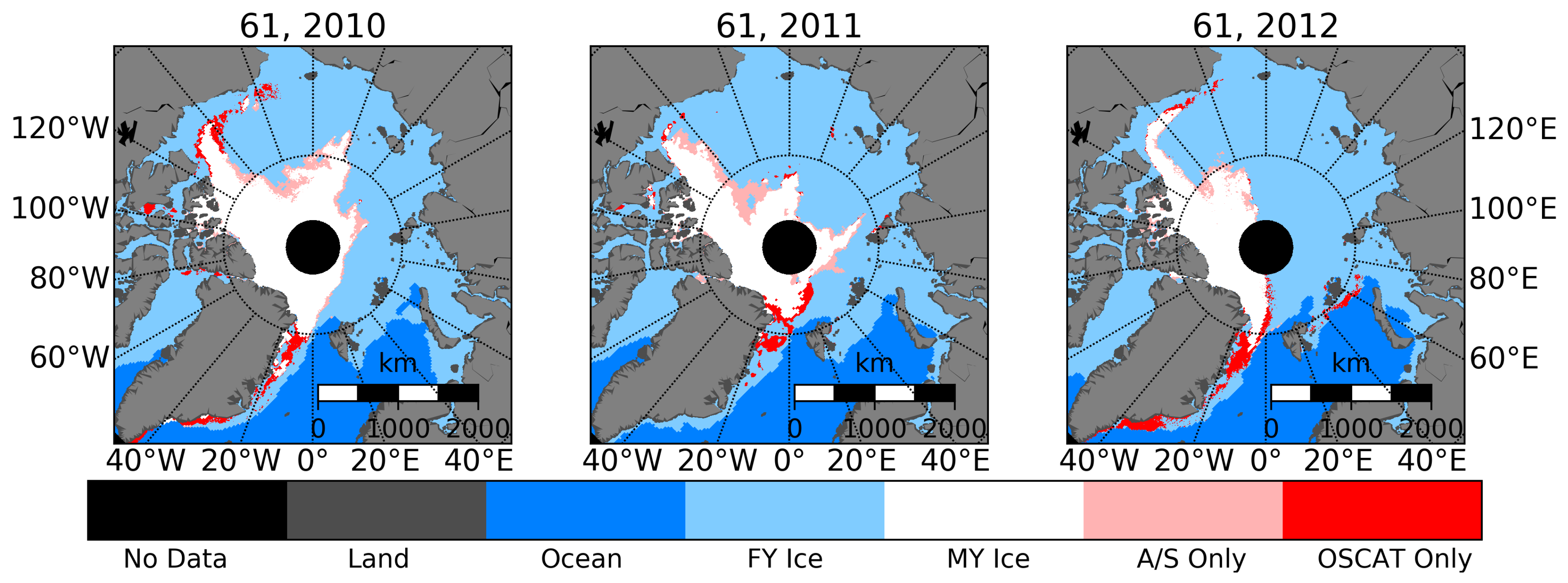
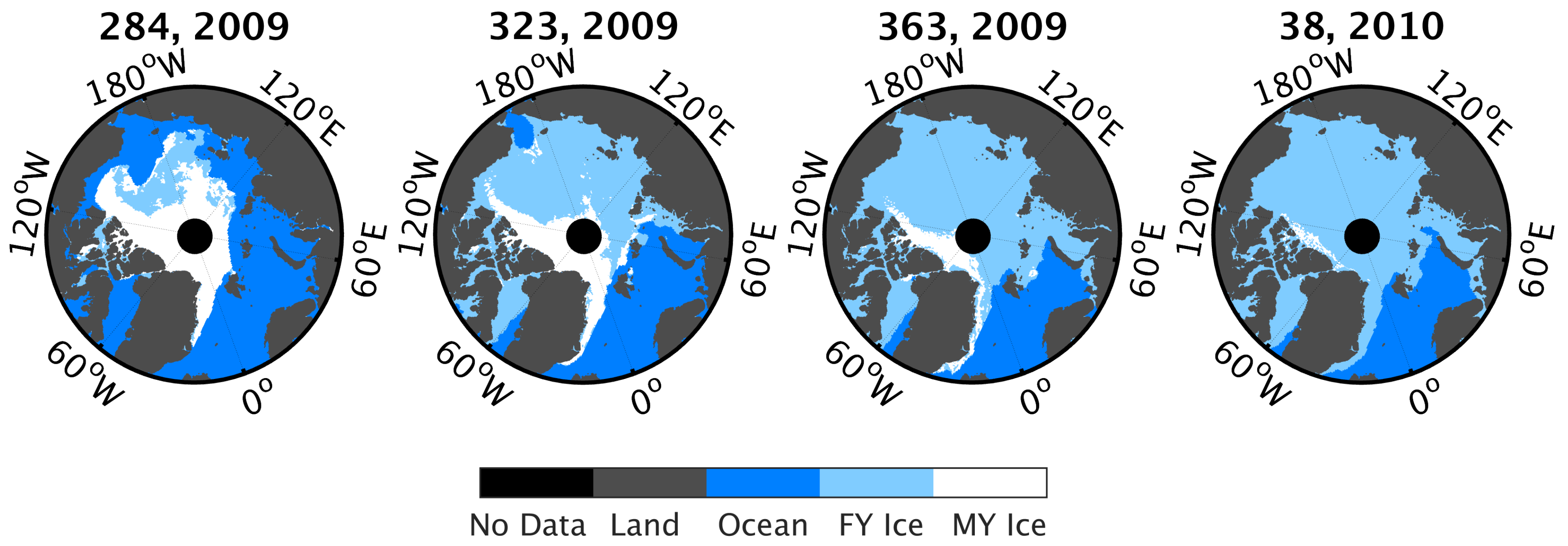
Example classification images for day of year 61 of years 2010, 2011, and 2012 are shown in Figure 4; we select this day of year arbitrarily because the images are representative of typical ASCAT/SSMIS classification results. The images also provide a comparison to the OSCAT classifications for the same days. Differences between the ASCAT/SSMIS and OSCAT classifications are occur noticeably in the central Arctic, in the Greenland Sea, and, in the 2012 image, near the sea ice edge at approximately 60 degrees east longitude.
In the central Arctic, the ASCAT/SSMIS classifications of MY ice frequently extend beyond the area classified with OSCAT. This difference may be due to a difference in the sensitivity of the classification algorithms to different concentrations of MY ice. To determine the typical concentration of MY ice for which an area of ice is classified as MY using ASCAT/SSMIS, we compare the ASCAT/SSMIS classifications to the CIS charts in an analysis described later in the section.
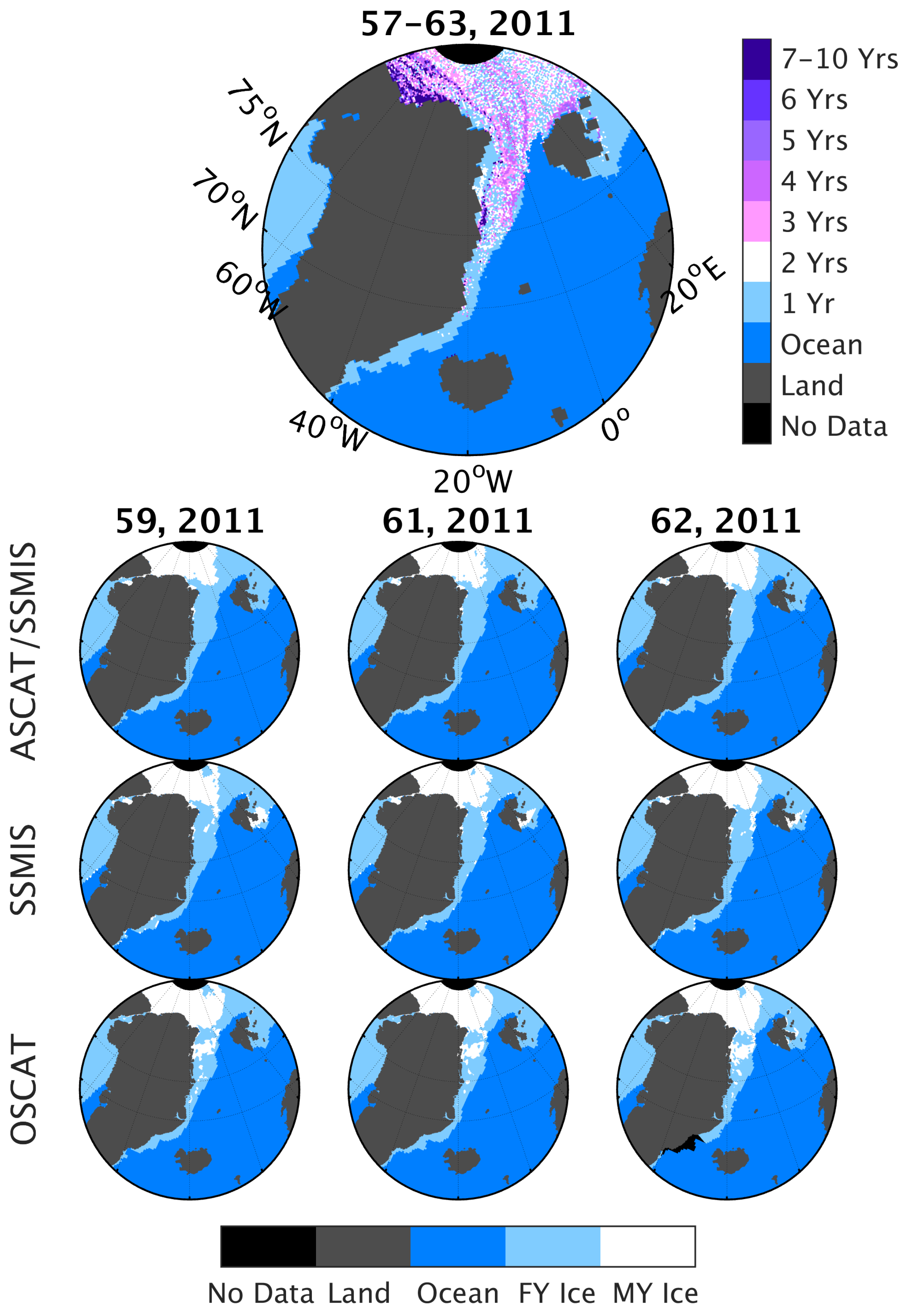
Differences also appear in Figure 4 near the east coast of Greenland, where the OSCAT classifications classify MY ice which is classified as FY with ASCAT/SSMIS. To investigate the classification differences in the Greenland Sea, classifications with ASCAT/SSMIS, SSMIS-only, OSCAT, and from the EASE-Grid Sea Ice Age product are analyzed for the time period around day of year 61, 2011. Figure 5 shows sample classification images for days of year 59, 61, and 62 (day of year 60 is omitted because of a gap in the OSCAT data). Within each classification method, the classifications appear to be consistent across the days shown, and only small changes are visible between days as expected. Note that while the EASE-Grid Sea Ice Age product reports large areas of MY ice extending south to approximately 75 degrees N latitude, only the OSCAT classifications classify large areas of MY ice south of approximately 81 degrees N latitude. The cause of the classification differences in the Greenland Sea is not readily apparent. It seems unlikely that the MIZ correction steps cause the differences because both the ASCAT/SSMIS classifications, which incorporate the correction steps, and the SSMIS-only classifications, which do not incorporate the correction steps, demonstrate similar behavior in the Greenland Sea. We are unable to determine the precise cause of the Greenland Sea classification differences, though the variability of Greenland sea ice composition and the ice fraction sensitivity differences between the classification algorithms are possible contributing factors.
On day of year 61, 2012, Figure 4 shows that the OSCAT classifications classify a patch of ice near the ice edge as MY ice despite the correction algorithm. When areas of high backscatter near the ice edge persist for several days, the effectiveness of the correction algorithm is decreased and such misclassifications can remain [2].
3.1. CIS Chart Comparison
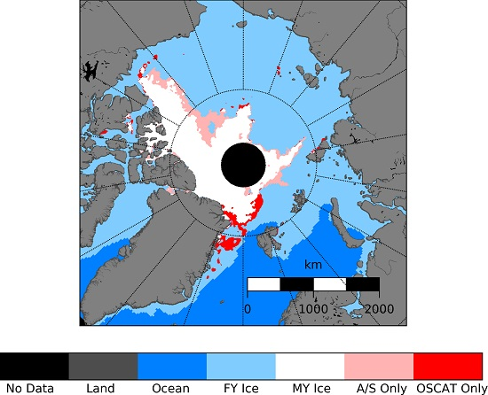
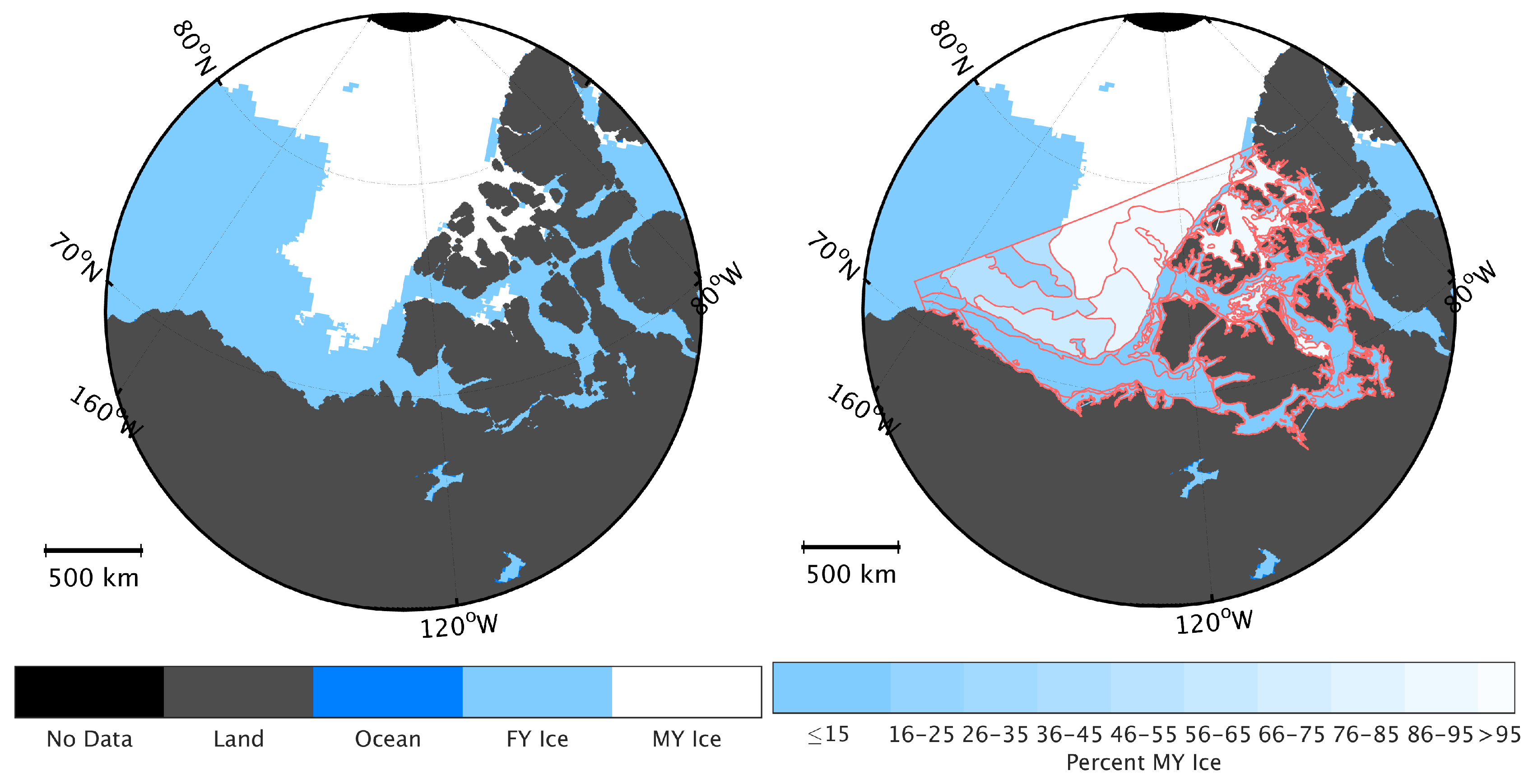
The ASCAT/SSMIS classifications are compared to the CIS charts for the region of the Western Arctic. Figure 6 shows the ASCAT/SSMIS classifications for arbitrarily selected day of year 2, 2011 and the same classifications with the CIS chart classifications from day of year 3, 2011 overlaid. As data for up to 72 h prior to the reported date are used to create the CIS charts, we choose a single-day offset for the comparison. In the figure, the CIS chart data indicate the fraction of MY ice derived from summing reported fractions of 2nd-year ice, MY ice, and old ice. The areas of same MY ice concentration in the CIS chart overlay are identified by a red outline. Visual comparison of the plots shows that the ASCAT/SSMIS classifications of MY ice correspond to areas of approximately 50% MY ice concentration or greater as indicated by the CIS chart data.
A further analysis is conducted using CIS chart data from 2010, 2011, and 2012 to estimate the probability that ice is classified as FY or MY for different ice fraction values. For days on which both ASCAT/SSMIS classifications and CIS chart classifications are available, pixels classified as MY ice using ASCAT/SSMIS are collocated with the CIS chart classifications of MY ice fraction and FY ice fraction to produce histograms of ASCAT/SSMIS MY ice pixel count and FY ice pixel count versus CIS chart MY and FY ice fraction. The histograms are normalized by the total pixel count of each MY/FY ice fraction histogram bin. The total pixel count is computed for each bin by adding the number of pixels in each bin classified as FY ice and as MY ice. The MY/FY ice fraction bin totals are rescaled so that they sum to one, forming a probability distribution. Using this method, the probability functions are also estimated for the SSMIS-only and OSCAT classifications.
The resulting probability distributions are shown in Figure 7. The figure shows that for most pixels classified as MY ice using ASCAT/SSMIS, the corresponding CIS chart concentrations of MY and FY ice are usually greater than 50% and less than 40%, respectively. FY ice classifications are approximately uniform in probability over FY ice fractions of 50% to 100% and MY ice fractions of 0% to 50%. The relationship between the MY and FY ice fraction classification probabilities is approximately inverse: where the FY ice fraction probabilities are large for MY ice classification, the FY ice fraction probabilities are small for FY ice classification, and the same for MY ice fraction probabilities. The inverse relationship results from the binary nature of the classifications. Overall, the classifiers appear to have a greater MY ice fraction threshold for MY ice classification than FY ice fraction threshold for FY ice classification.
The probability plots also demonstrate differences in behavior between the ASCAT/SSMIS, SSMIS-only, and OSCAT classifications. The ASCAT/SSMIS classifications appear to be the most restrictive in that they classify ice of a lower MY ice fraction as MY less often than the other classifiers. The SSMIS-only classifications are similar to the ASCAT/SSMIS classifications, though they classify more MY ice areas of a low MY ice fraction. The OSCAT classifications demonstrate a sharper MY ice classification threshold than ASCAT/SSMIS or SSMIS-only, with a lower probability of classifying MY ice in areas with a MY ice fraction lower than 60%.
3.2. Ice Extent Time Series
A time series of total ice extent and MY ice extent from ASCAT/SSMIS, SSMIS only, OSCAT, and the EASE-Grid Sea Ice Age datasets is shown in Figure 8. In each case, the MY ice extent is determined by summing the area of grid cells classified as MY ice. Similarly to [2], we do not include grid cells of the pole hole (black disc in Figure 4), which extends from 87 to 90 degrees N latitude over an area of 364 thousand km. The grid area for each pixel is determined using the Scatterometer Image Reconstruction grid area file for the north polar stereographic projection. The area file is available from the Scatterometer Climate Record Pathfinder FTP site [30]. As a measure of the uncertainty in the classifications, we calculate the standard deviation of the MY ice extent values for ASCAT/SSMIS using a sliding window of 60 days of extent values. The standard deviation values are too small to be easily observed on the plot, and so are not included. The average value of the calculated standard deviations is 192 thousand km with a standard deviation of 80 thousand km. The 60-day window standard deviation values are typically lower (around 100 to 160 thousand km) during the beginning of winter and then may increase to between 250 and 350 thousand km in the middle of winter and again at the very end of winter.
In the EASE-Grid Sea Ice Age dataset, the age of sea ice is classified by year using integer values from one to ten. MY ice areas including (EASE 2+) and excluding (EASE 3+) second-year ice are identified by summing the area of all grid cells classified with a value of two or greater and three or greater. Again, grid cells within the pole hole are omitted. Both EASE-Grid Sea Ice Age groups are included for comparison with the ASCAT/SSMIS, SSMIS-only, and OSCAT ice classifications. We note that the EASE-Grid Sea Ice Age data are available only through 2012, so data for years after are not included.
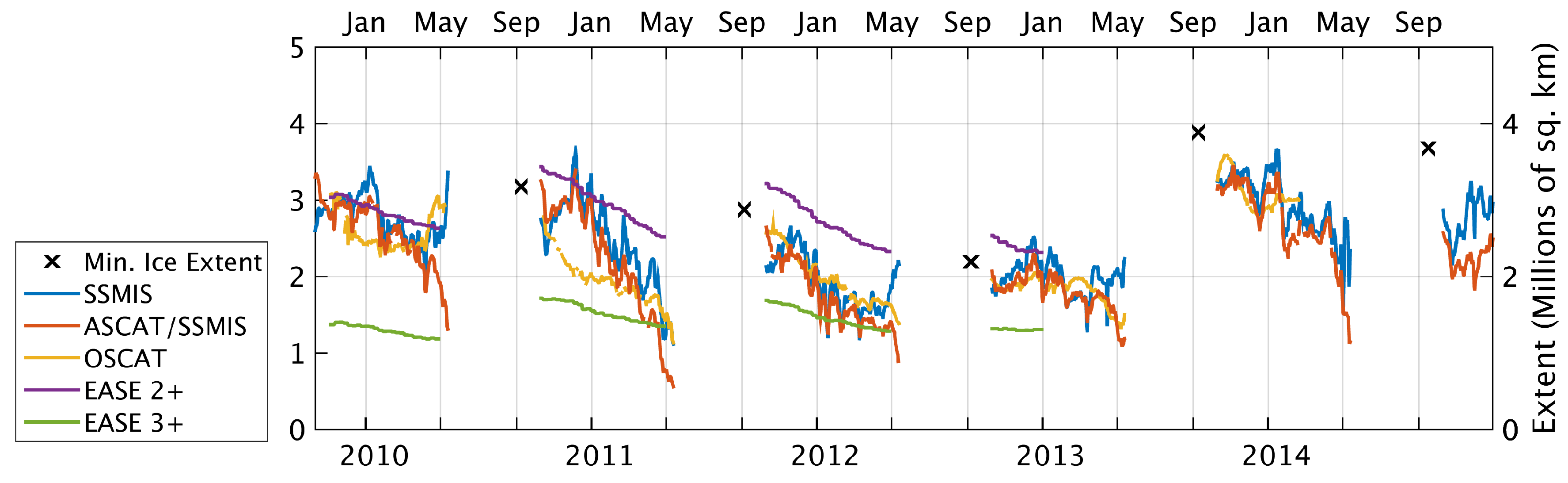
The total extent of MY ice appears to decrease from the winters of 2009 to 2013, followed by a recovery in 2014. Other studies have similarly reported a decline in MY ice [2,11] and recovery in 2014 [45]. Total MY ice extent levels appear to follow roughly the same cycle from the winters of 2009 to 2013. Following the winter of 2012/2013, MY ice extent levels do not drop to the low levels observed in previous years (below 1 million km), and vary from approximately 2 to 3.5 million km during the majority of the winter. From 2009 to 2014, the MY ice extent of the ASCAT/SSMIS classifications demonstrates an average difference of 282 thousand km from that of the OSCAT classifications. The difference is an average of 13.6% of the OSCAT MY ice extent, which averaged 2.19 million km over the same period. Compared to the EASE-2+ classifications from 2009 to 2012, the average difference is 617 thousand km. The difference is an average of 22.8% of the EASE-2+ MY ice extent, which averaged 2.79 million km from 2009 to 2012.
In Figure 8, the ASCAT/SSMIS classifications show general agreement with the OSCAT classifications, though some differences are apparent, including during the winters of 2009/2010 and 2010/2011 and near the end of each winter. Also, at the beginning of winters, increases in MY ice extent appear, followed by a decrease. An increase in MY ice area is not physically supported as new MY ice is not created during the winter, rather the area of MY ice decreases.
During the first two winters shown in Figure 7, the differences in MY ice extent are mainly due to a difference in ice classifications in the central Arctic where more MY ice is classified with ASCAT/SSMIS than with OSCAT. Near the end of winter, the ASCAT/SSMIS classifications tend to drop sharply in MY ice extent and become more sporadic, with large changes in the classifications from day to day. The rapid decline in the extent of classified MY ice could result from changing microwave signatures of ice at the onset of the summer melt.
The MY ice extent increases during the beginning of winter could correspond to areas of high MY ice concentration becoming spread out during events of divergent sea ice motion, resulting in greater areas of diffuse MY ice, which continue to be classified as MY ice with ASCAT/SSMIS. Though the area of MY ice does not increase throughout the winter, the extent of MY ice could increase through such a process. Other factors which cause FY ice to appear similar to MY ice could contribute to an increased area of MY ice classification. Such factors include deformation of FY ice, which can increase at C-band due to the increase in surface roughness [23], and deep snow, which can cause a decrease in brightness temperature at 37 GHz [28]. Note that the 37 GHz and 18 or 19 GHz channels (V) have been used to retrieve snow depth on FY ice [46,47]. More work is required to determine the precise physical cause of the MY extent increase at the beginning of winter.
The variability in the MY ice extent of the ASCAT/SSMIS classifications may be caused by the changing parameters of the Bayesian classifier, which result in greater variation of the FY/MY boundary than for the ice motion vector tracking method of the EASE-Grid Sea Ice Age product. ASCAT/SSMIS classifications in the Greenland Sea can change rapidly from day to day and contribute to the variability observed in the MY ice extent. Further investigation of the classification algorithm is required to determine the cause of the variability.
The SSMIS-only classifications appear very similar to the ASCAT/SSMIS classifications, which suggests that ASCAT data does not add too much new information. Comparing the MY ice extents of the two classification methods in Figure 8 shows that the ASCAT/SSMIS classifications are slightly less variable in some periods and tend not to increase at the end of the year as the SSMIS-only classifications do in a few cases. A zoom-in comparison of classifications for day of year 2, 2011 in Figure 9 shows a similar MY ice extent, but some finer resolution details are present in the ASCAT/SSMIS classifications which are not present in the SSMIS-only classifications.
The addition of SSMIS passive data is useful because it not only provides more information for the Bayesian classifier, but also helps to compensate for the sensitivity of ASCAT to areas of broken ice near the ice edge and reduce misclassification of ice. Using ASCAT data alone results in large areas of misclassified ice near the ice edge that skew the Bayesian classification parameters as they are updated using previous classifications, resulting in greater and greater amounts of error. A series of ASCAT-only classification images are shown in Figure 10 and shows that the classifications classify a lesser and lesser area of MY ice until nearly all of the ice is classified as FY. Similar results are not observed when including the SSMIS data.
Differences between the ASCAT/SSMIS, SSMIS-only, OSCAT, and EASE-Grid ice classifications can be evaluated by noting that the area of MY ice should decrease over the winter and drawing comparisons between the rate of decrease in the EASE-Grid product and in the other classifications. In the following, we note some observed trends and reflect on possible causes. (1) For the winter of 2009/2010, the ASCAT/SSMIS and SSMIS-only classifications show better agreement with the EASE-2+ MY extent than with EASE-3+ and are close in value to the OSCAT MY extent; (2) During 2010/2011, ASCAT/SSMIS and SSMIS-only remain similar to EASE-2+ over the first half of the winter, but then rapidly decline in MY extent. During the same period, OSCAT shows a decline in MY extent similar to EASE-3+; (3) For the winters of 2011/2012, 2012/2013, and 2013/2014, the ASCAT/SSMIS and SSMIS-only MY extent are more comparable to the OSCAT MY extent, which tends to approximate EASE-3+ more than EASE-2+ in terms of value and the pace of the MY ice decrease over each winter.
During the winters of 2009/2010, the ASCAT/SSMIS, SSMIS-only, and OSCAT MY extent appears to follow the EASE-2+ pace of extent decrease, though at the end of the winter, the SSMIS-only and OSCAT MY extent demonstrates an increase which appears to be caused by melt effects; the ASCAT/SSMIS extent shows a sharp decrease as classifications become sporadic from day to day, possibly also because of melt effects.
Over the 2010/2011 winter, the OSCAT MY extent shows greater agreement with EASE-3+ while ASCAT/SSMIS and SSMIS-only exhibit a sharper decline in MY extent than EASE-2+ or EASE-3+. The rapid decline in MY extent for ASCAT/SSMIS and SSMIS-only appears to be caused by changing classifications in the Greenland Sea. For the first half of the winter, nearly all of the ice in the Greenland Sea is classified as MY; near the end of the winter, the Greenland Sea classifications become quite variable and then begin to decrease rapidly in MY extent, leading to the rapid decline observed in the total MY extent.
During the following winters of 2011/2012, 2012/2013, and 2013/2014, the ASCAT/SSMIS and SSMIS-only MY extents generally agree with the OSCAT MY extent. During these winters, the ASCAT/SSMIS and SSMIS-only classifications typically show better agreement with OSCAT during the first half of the winter than for the second half. For the winter period of 2011/2012, the MY extent in the central Arctic closely follows the OSCAT MY extent, but the total MY extent begins to demonstrate greater differences after the beginning of 2012. While the OSCAT classifications continue to classify MY ice in the Greenland Sea during the beginning of 2012, the ASCAT/SSMIS classifications demonstrate a decline in the area of classified MY ice in the Greenland Sea, leading to the observed MY extent differences. Similar trends are observed for the winters of 2012/2013 and 2013/2014 where the ASCAT/SSMIS MY extent agrees with the OSCAT extent for the first half of the winter before decreasing in the second half due to a decline in classified MY ice in the Greenland Sea. This phenomenon is prominently displayed by the strong decline in MY ice extent at the beginning of 2014. Overall, the rate of decline in the ASCAT/SSMIS MY extent in the central Arctic is comparable to both OSCAT and EASE-3+.
4. Conclusions
Using a fusion of active and passive microwave data, FY and MY ice can be classified in the Arctic. Comparison of ASCAT/SSMIS classifications to the CIS charts shows that areas of approximately 50% or greater MY ice concentration in the CIS charts are typically classified as MY ice in the ASCAT/SSMIS classifications. The extent of classified MY ice in the ASCAT/SSMIS classifications generally agrees with that of OSCAT and demonstrates comparable declines in MY extent over the winter to what is observed in the EASE-2+ and EASE-3+ classifications. Differences between the ASCAT/SSMIS and OSCAT or EASE-2+/EASE-3+ classifications arise from the variability of the ASCAT/SSMIS classifications in the Greenland Sea and from an increase in ASCAT/SSMIS MY extent which occurs at the beginning of winters. As the cause of classification differences in the Greenland sea is not apparent at this point; further investigation of the classification algorithm performance in that area could be performed. More investigation is also required to determine the physical cause of the increase in MY extent observed at the beginning of winters. Though the area of MY ice should not increase throughout the winter, the extent increase of MY ice may be caused areas of high MY ice concentration becoming spread out during events of divergent sea ice motion, resulting in a greater area of diffuse MY ice, which continues to be classified as MY ice with ASCAT/SSMIS. The overall variability in the ASCAT/SSMIS MY extent may be caused by the variation in the parameters of the Bayesian classifier, which might vary substantially during the course of the winter.
The addition of the passive SSMIS data appears to improve classifications by mitigating misclassifications caused by ASCAT’s sensitivity to rough patches of ice which can appear similar to, but are not, MY ice. As the ASCAT and SSMIS sensors continue to operate, future work could be done to reduce the variability in the MY ice extent of the classifications and to improve classification of MY ice outside the main area of MY ice, especially in the Greenland Sea.
Acknowledgments
The authors are grateful to the CIS, NSIDC, JPL PODAAC, and SCP for providing data used in the paper. They also thank the anonymous reviewers for their helpful comments.
Author Contributions
David Lindell processed the data and wrote the manuscript with advice and guidance from David Long.
Conflicts of Interest
The authors declare no conflict of interest.
References
- Swan, A.; Long, D. Multiyear Arctic sea ice classification using QuikSCAT. IEEE Trans. Geosci. Remote Sens. 2012, 50, 3317–3326. [Google Scholar] [CrossRef]
- Lindell, D.; Long, D. Multiyear Arctic sea ice classification using OSCAT and QuikSCAT. IEEE Trans. Geosci. Remote Sens. 2016, 54, 167–175. [Google Scholar] [CrossRef]
- Kwok, R. Annual cycles of multiyear sea ice coverage of the Arctic Ocean: 1999–2003. J. Geophys. Res. 2004, 109. [Google Scholar] [CrossRef]
- Kwok, R.; Rignot, E.; Holt, B.; Onstott, R. Identification of sea ice types in spaceborne synthetic aperture radar data. J. Geophys. Res. 1992, 97, 2391–2402. [Google Scholar] [CrossRef]
- Nghiem, S.; Bertoia, C. Study of multi-polarization C-band backscatter signatures for Arctic sea ice mapping with future satellite SAR. Can. J. Remote Sens. 2001, 27, 387–402. [Google Scholar] [CrossRef]
- Zakhvatkina, N.; Alexandrov, V.; Johannessen, O.; Sandven, S.; Frolov, I. Classification of sea ice types in ENVISAT synthetic aperture radar images. IEEE Trans. Geosci. Remote Sens. 2013, 51, 2587–2600. [Google Scholar] [CrossRef]
- Casey, J.A.; Howell, S.E.; Tivy, A.; Haas, C. Separability of sea ice types from wide swath C-and L-band synthetic aperture radar imagery acquired during the melt season. Remote Sens. Environ. 2016, 174, 314–328. [Google Scholar] [CrossRef]
- Comiso, J. Arctic multiyear ice classification and summer ice cover using passive microwave satellite data. J. Geophys. Res. 1990, 95, 13411–13422. [Google Scholar] [CrossRef]
- Lomax, A.; Lubin, D.; Whritner, R. The potential for interpreting total and multiyear ice concentrations in SSM/I 85.5 GHz imagery. Remote Sens. Environ. 1995, 54, 13–26. [Google Scholar] [CrossRef]
- Belchansky, G.; Douglas, D.; Platonov, N. Spatial and temporal variations in the age structure of Arctic sea ice. Geophys. Res. Lett. 2005, 32. [Google Scholar] [CrossRef]
- Comiso, J. Large decadal decline of the Arctic multiyear ice cover. J. Clim. 2012, 25, 1176–1193. [Google Scholar] [CrossRef]
- Cavalieri, D. NASA Team Sea Ice Algorithm. Available online: http://nsidc.org/data/docs/daac/nasateam/ (accessed on 28 March 2016).
- Comiso, J. SSM/I Concentration Using the Bootstrap Algorithm; NASA Report 1380; NASA Center for Aerospace Information: Linthicum Heights, MD, USA, 1995. [Google Scholar]
- Shokr, M.; Agnew, T. Validation and potential applications of Environment Canada Ice Concentration Extractor (ECICE) algorithm to Arctic ice by combining AMSR-E and QuikSCAT observations. Remote Sens. Environ. 2013, 128, 315–332. [Google Scholar] [CrossRef]
- Yu, P.; Clausi, D.; Howell, S. Fusing AMSR-E and QuikSCAT imagery for improved sea ice recognition. IEEE Trans. Geosci. Remote Sens. 2009, 47, 1980–1989. [Google Scholar] [CrossRef]
- Walker, N.; Partington, K.; Van Woert, M.; Street, T. Arctic sea ice type and concentration mapping using passive and active microwave sensors. IEEE Trans. Geosci. Remote Sens. 2006, 44, 3574–3584. [Google Scholar] [CrossRef]
- Screen, J.; Simmonds, I.; Deser, C.; Tomas, R. The atmospheric response to three decades of observed Arctic sea ice loss. J. Clim. 2013, 26, 1230–1248. [Google Scholar] [CrossRef]
- Liu, J.; Curry, J.A.; Wang, H.; Song, M.; Horton, R. Impact of declining Arctic sea ice on winter snowfall. Proc. Natl. Acad. Sci. USA 2012, 109, 4074–4079. [Google Scholar] [CrossRef] [PubMed]
- Kwok, R.; Spreen, G.; Pang, S. Arctic sea ice circulation and drift speed: Decadal trends and ocean currents. J. Geophys. Res. Oceans 2013, 118, 2408–2425. [Google Scholar] [CrossRef]
- Maslanik, J.; Stroeve, J.; Fowler, C.; Emery, W. Distribution and trends in Arctic sea ice age through spring 2011. Geophys. Res. Lett. 2011, 38, L13502. [Google Scholar] [CrossRef]
- Schweiger, A.; Lindsay, R.; Zhang, J.; Steele, M.; Stern, H.; Kwok, R. Uncertainty in modeled Arctic sea ice volume. J. Geophys. Res. Oceans 2011, 116, C00D06. [Google Scholar] [CrossRef]
- Laxon, S.W.; Giles, K.A.; Ridout, A.L.; Wingham, D.J.; Willatt, R.; Cullen, R.; Kwok, R.; Schweiger, A.; Zhang, J.; Haas, C.; et al. CryoSat-2 estimates of Arctic sea ice thickness and volume. Geophys. Res. Lett. 2013, 40, 732–737. [Google Scholar] [CrossRef]
- Rivas, M.; Verspeek, J.; Verhoef, A.; Stoffelen, A. Bayesian sea ice detection with the Advanced Scatterometer ASCAT. IEEE Trans. Geosci. Remote Sens. 2012, 50, 2649–2657. [Google Scholar] [CrossRef]
- Mortin, J.; Howell, S.; Wang, L.; Derksen, C.; Svensson, G.; Graversen, R.; Schrøder, T. Extending the QuikSCAT record of seasonal melt–freeze transitions over Arctic sea ice using ASCAT. Remote Sens. Environ. 2014, 141, 214–230. [Google Scholar] [CrossRef]
- Rivas, M.B.; Stoffelen, A. New Bayesian Algorithm for sea ice detection with QuikSCAT. IEEE Trans. Geosci. Remote Sens. 2011, 49, 1894–1901. [Google Scholar] [CrossRef]
- Onstott, R.G. SAR and scatterometer signatures of sea ice. In Microwave Remote Sensing of Sea Ice; Carsey, F.D., Ed.; American Geophysical Union: Washington, DC, USA, 1992. [Google Scholar] [CrossRef]
- Shokr, M.E. Field observations and model calculations of dielectric properties of Arctic sea ice in the microwave C-band. IEEE Trans. Geosci. Remote Sens. 1998, 36, 463–478. [Google Scholar] [CrossRef]
- Eppler, D.; Farmer, L.; Lohanick, A.; Anderson, M.; Cavalieri, D.; Comiso, J.; Glorsen, P.; Garrity, C.; Grenfell, T.; Hallikainen, M.; et al. Passive microwave signatures of sea ice. In Microwave Remote Sensing of Sea Ice; Carsey, F.D., Ed.; American Geophysical Union: Washington, DC, USA, 1992. [Google Scholar] [CrossRef]
- Vant, M.; Ramseier, R.; Makios, V. The complex-dielectric constant of sea ice at frequencies in the range 0.1–40 GHz. J. Appl. Phys. 1978, 49, 1264–1280. [Google Scholar] [CrossRef]
- Scatterometer Climate Record Pathfinder. Available online: http://www.scp.byu.edu/ (accessed on 28 March 2016).
- Cavalieri, D.; Parkinson, C.; Gloersen, P.; Zwally, H. Sea Ice Concentrations from Nimbus-7 SMMR and DMSP SSM/I-SSMIS Passive Microwave Data. Available online: http://dx.doi.org/10.5067/8GQ8LZQVL0VL (accessed on 28 March 2016).
- Lindsley, R. Estimating the ASCAT Spatial Response Function; Technical Report 14-01; BYU MERS Lab: Provo, UT, USA, 2014; Available online: http://www.mers.byu.edu/docs/reports/MERS1401.pdf (accessed on 28 March 2016).
- Lindsley, R.; Long, D. A parameterized ASCAT measurement spatial response function. IEEE. Trans. Geosci. Remote Sens. 2016. submitted. [Google Scholar]
- Maslanik, J.; Stroeve, J. DMSP SSM/I-SSMIS Daily Polar Gridded Brightness Temperatures. National Snow and Ice Data Center: Boulder, CO; Available online: http://nsidc.org/data/nsidc-0001/ (accessed on 28 March 2016).
- Long, D.G.; Daum, D.L. Spatial resolution enhancement of SSM/I data. IEEE Trans. Geosci. Remote Sens. 1998, 36, 407–417. [Google Scholar] [CrossRef]
- Long, D.; Hardin, P.; Whiting, P. Resolution enhancement of spaceborne scatterometer data. IEEE Trans. Geosci. Remote Sens. 1993, 31, 700–715. [Google Scholar]
- Lindsley, R.D.; Long, D.G. Enhanced-resolution reconstruction of ASCAT backscatter measurements. IEEE Trans. Geosci. Remote Sens. 2015, 54, 2589–2601. [Google Scholar]
- Cavalieri, D.; Parkinson, C.; DiGirolamo, N.; Ivanoff, A. Intersensor calibration between F13 SSMI and F17 SSMIS for global sea ice data records. IEEE Geosci. Remote Sens. Lett. 2012, 9, 233–236. [Google Scholar]
- Tschudi, M.; Fowler, C.; Maslanik, J. EASE-Grid Sea Ice Age [2009–2012]. Available online: http://dx.doi.org/10.5067/1UQJWCYPVX61 (accessed on 28 March 2016).
- Canadian Ice Service Arctic Regional Sea Ice Charts in SIGRID-3 Format, Version 1. [2010–2012]. Available online: http://dx.doi.org/10.7265/N51V5BW9 (accessed on 28 March 2016).
- Fowler, C.; Emery, W.J.; Maslanik, J. Satellite-derived evolution of Arctic sea ice age: October 1978 to March 2003. IEEE Geosci. Remote Sens. Lett. 2004, 1, 71–74. [Google Scholar] [CrossRef]
- Tschudi, M.; Fowler, C.; Maslanik, J.; Stroeve, J. Tracking the movement and changing surface characteristics of Arctic sea ice. IEEE J. Sel. Top. Appl. Earth Obs. Remote Sens. 2010, 3, 536–540. [Google Scholar]
- Kwok, R.; Schweiger, A.; Rothrock, D.A.; Pang, S.; Kottmeier, C. Sea ice motion from satellite passive microwave imagery assessed with ERS SAR and buoy motions. J. Geophys. Res. Oceans 1998, 103, 8191–8214. [Google Scholar]
- MANICE. Manual of Standard Procedures for Observing and Reporting Ice Conditions; Technical report; Environment Canada: Ottawa, ON, Canada, 2005. [Google Scholar]
- Tilling, R.; Ridout, A.; Shepherd, A.; Wingham, D. Increased Arctic sea ice volume after anomalously low melting in 2013. Nat. Geosci. 2015, 8, 643–646. [Google Scholar] [CrossRef]
- Markus, T.; Cavalieri, D.J. Snow depth distribution over sea ice in the Southern Ocean from satellite passive microwave data. In Antarctic Sea Ice: Physical Processes, Interactions and Variability; Jeffries, M.O., Ed.; American Geophysical Union: Washington, DC, USA, 1998; pp. 19–39. [Google Scholar]
- Cavalieri, D.J.; Markus, T.; Ivanoff, A.; Miller, J.A.; Brucker, L.; Sturm, M.; Maslanik, J.A.; Heinrichs, J.F.; Gasiewski, A.J.; Leuschen, C.; et al. A comparison of snow depth on sea ice retrievals using airborne altimeters and an AMSR-E simulator. IEEE Trans. Geosci. Remote Sens. 2012, 50, 3027–3040. [Google Scholar] [CrossRef]
Figure 1.
Time series of daily histograms for QuikSCAT (top row) for the winters of 2000/2001 and 2001/2002 and ASCAT (bottom row) for the winters of 2010/2011 and 2011/2012. The QuikSCAT distribution demonstrates a separation of modes corresponding to FY ice and MY ice, whereas the ASCAT distribution does not clearly demonstrate such separation. Each histogram in the time series is normalized by its maximum bin count.

Figure 2.
Example images of ASCAT values and brightness temperatures for day of year 61, 2011 from the 37 GHz (V) channel of SSMIS over the Arctic. Areas of open water and land are masked as light yellow or black, respectively. The areas of MY ice correspond generally to the areas of high values and low brightness temperature () values.

Figure 3.
Joint scatterplots/2D histograms of ASCAT values and SSMIS brightness temperatures () for day of year 61, 2011. When the density of the scatterplot becomes too great to be able to discern individual points, the density is shown in a 2D histogram. For the 2D histogram, bin sizes are 0.5 dB by 1 K. Scatterplots/2D histograms of MY ice, FY ice, and both (all ice) are shown from left to right. The distributions of brightness temperatures and corresponding to FY and MY ice are derived using the OSCAT ice type classifications [2].

Figure 4.
Example ice classification images from day of year 61 for years 2010, 2011, and 2012. The ASCAT/SSMIS classifications are compared to the OSCAT classifications and the differences are highlighted. Areas classified as MY in the ASCAT/SSMIS classifications but not by OSCAT are highlighted in pink. Areas classified as MY in the OSCAT classifications but not by ASCAT/SSMIS are highlighted in red.

Figure 5.
Collection of ice classifications from the EASE-Grid Sea Ice Age product (top), ASCAT/SSMIS (second row), SSMIS (third row), and OSCAT (fourth row). The EASE-Grid product is provided weekly and is here shown for days of year 57 to 63, 2011. The other classification images are shown for days of year 59, 61, and 62, 2011. Data from day of year 60 are omitted because of a gap in the OSCAT data.

Figure 6.
Images of ASCAT/SSMIS ice classifications for day of year 2, 2011 (left), and CIS chart classifications for day of year 3, 2011 overlaid on the ASCAT/SSMIS classifications (right). The data dates are offset because CIS charts are constructed using data retrieved up to 72 h prior to the reported date. In the right image, areas of the same CIS chart classification are enclosed by a red line.

Figure 7.
Probability distributions of ice classified as MY (top) and FY (bottom) with ASCAT/SSMIS (left), SSMIS-only (middle), and OSCAT (right) versus the CIS chart fractions of FY and MY ice. Most ASCAT/SSMIS pixels classified as MY ice (MYI) correspond to a MYI fraction of approximately 50% or greater and a FY ice (FYI) fraction of approximately 40% or less in the CIS charts.

Figure 8.
Time series of minimum total ice extent and MY ice extent. Plots are shown of the MY ice extent from SSMIS-only, ASCAT/SSMIS, and OSCAT ice classifications, as well as the extent of old ice including (EASE 2+) and excluding (EASE 3+) second-year ice as taken from the NSIDC EASE-Grid Sea Ice Age dataset. The annual total ice extent minima are calculated using a 40% ice concentration ice edge as reported by a NASA Team ice concentration product [31]. The average standard deviation for the ASCAT/SSMIS MY extent over 60-day windows is 192 thousand km.

Figure 9.
Zoom-in comparison of ASCAT/SSMIS and SSMIS-only ice classifications for day of year 2, 2011. In some areas, the ASCAT/SSMIS classifications contain finer details than the SSMIS classifications because of the inclusion of enhanced-resolution ASCAT data.
Figure 9.
Zoom-in comparison of ASCAT/SSMIS and SSMIS-only ice classifications for day of year 2, 2011. In some areas, the ASCAT/SSMIS classifications contain finer details than the SSMIS classifications because of the inclusion of enhanced-resolution ASCAT data.

Figure 10.
Time series of ice classification images produced using ASCAT data only for the winter of 2009/2010. Images are labeled according to day of year and year. Misclassifications of ice near the ice edge result in increasing classification errors until nearly all ice is classified as FY.
Figure 10.
Time series of ice classification images produced using ASCAT data only for the winter of 2009/2010. Images are labeled according to day of year and year. Misclassifications of ice near the ice edge result in increasing classification errors until nearly all ice is classified as FY.


Table 1.
Characteristics of the Advanced Scatterometer (ASCAT) and Special Sensor Microwave Imager/Sounder (SSMIS).
| Parameter | ASCAT | SSMIS |
|---|---|---|
| Organization | European Organization for the | Defense Meteorological |
| Exploitation of Meteorological | Satellite | |
| Satellites (EUMETSAT) | Program (DMSP) | |
| Frequency Channels | 5.255 GHz (V-pol) | 37 GHz (V-pol) * |
| Orbital Period | 101 min | 102 min (F-17) |
| Orbital Inclination | 98.7 | 98.8 |
| Ascending Node Local Time | 9:30 p.m. | 5:31 p.m. |
| Satellite Altitude | 817 km | 850 km |
| Start Date | 19 October 2006 | 4 November 2006 |
| Incidence Angle | Various | 53.1 degrees |
| Swath Width | Two 500 km-wide | 1707 km |
| swaths separated by a 360 km-wide | ||
| nadir gap | ||
| Footprint Size | ≈ 19–35 km × 500 km | 70 × 45 km (19.35 GHz) |
| 38 × 30 km (37 GHz) | ||
| Image Resolution | 4.45 km per pixel | 25 km per pixel |
* Frequency channel and polarization used in this paper. SSMIS has frequency channels ranging from 19.35 to 183.311 GHz at various polarizations. Area illuminated by the fan beam. Range-Doppler processing results in measurements from smaller footprints within the total illuminated area. The size of and shape of the range-Doppler footprints vary across the swath but are generally elliptical with dimensions to the −3 dB level on the order of 5 × 40 km [32,33]. Enhanced-resolution (4.45 km per pixel) data are obtained from the Scatterometer Climate Record Pathfinder [30] and are provided as daily postings of two-day averaged data normalized to 40 degrees incidence angle.
| Frequency | Polarization | Ice Type | Brightness Temperature |
|---|---|---|---|
| 19 GHz | V | FY | 258.2 K |
| MY | 223.2 K | ||
| H | FY | 242.8 K | |
| MY | 203.9 K | ||
| 37 GHz | V | FY | 252.8 K |
| MY | 186.3 K |
© 2016 by the authors; licensee MDPI, Basel, Switzerland. This article is an open access article distributed under the terms and conditions of the Creative Commons by Attribution (CC-BY) license (http://creativecommons.org/licenses/by/4.0/).
Share and Cite
MDPI and ACS Style
Lindell, D.B.; Long, D.G. Multiyear Arctic Ice Classification Using ASCAT and SSMIS. Remote Sens. 2016, 8, 294. https://doi.org/10.3390/rs8040294
AMA Style
Lindell DB, Long DG. Multiyear Arctic Ice Classification Using ASCAT and SSMIS. Remote Sensing. 2016; 8(4):294. https://doi.org/10.3390/rs8040294
Chicago/Turabian StyleLindell, David B., and David G. Long. 2016. "Multiyear Arctic Ice Classification Using ASCAT and SSMIS" Remote Sensing 8, no. 4: 294. https://doi.org/10.3390/rs8040294
Note that from the first issue of 2016, this journal uses article numbers instead of page numbers. See further details here.