The Impact of Geophysical Corrections on Sea-Ice Freeboard Retrieved from Satellite Altimetry

Abstract

Satellite altimetry is the only method to monitor global changes in sea-ice thickness and volume over decades. Such missions (e.g., ERS, Envisat, ICESat, CryoSat-2) are based on the conversion of freeboard into thickness by assuming hydrostatic equilibrium. Freeboard, the height of the ice above the water level, is therefore a crucial parameter. Freeboard is a relative quantity, computed by subtracting the instantaneous sea surface height from the sea-ice surface elevations. Hence, the impact of geophysical range corrections depends on the performance of the interpolation between subsequent leads to retrieve the sea surface height, and the magnitude of the correction. In this study, we investigate this impact by considering CryoSat-2 sea-ice freeboard retrievals in autumn and spring. Our findings show that major parts of the Arctic are not noticeably affected by the corrections. However, we find areas with very low lead density like the multiyear ice north of Canada, and landfast ice zones, where the impact can be substantial. In March 2015, 7.17% and 2.69% of all valid CryoSat-2 freeboard grid cells are affected by the ocean tides and the inverse barometric correction by more than 1 cm. They represent by far the major contributions among the impacts of the individual corrections.

1. Introduction

There is notable evidence for the thinning of the Arctic sea ice and thus a loss of sea-ice volume during the last decades [1,2,3,4]. Given that marine ice strongly modifies the exchange of energy and gases between the ocean and atmosphere and that these exchanges are important components of global climate, it is crucial that we continuously monitor sea-ice thickness and concurrently improve our thickness retrievals. Several past satellite missions (e.g., ICESat, ERS and Envisat) have demonstrated that altimetry offers great potential in monitoring sea-ice thickness but also showed considerable uncertainties [5]. In contrast to the lateral extent, thickness cannot be observed directly. The first step to retrieve sea-ice thickness is to determine the sea-ice freeboard, the height of the sea-ice surface above the sea level. Therefore, an accurate sea-surface height retrieval at the time of the satellite overflight is important. The instantaneous sea-surface height can be formulated as the sum of a mean sea-surface height ($MSS$) and a sea-surface anomaly ($SSA$) that represents the actual state of the sea level, including tides as well as local anomalies (e.g., eddies). The instantaneous sea-surface height can be retrieved by interpolating between elevations of detected leads, which are openings in the ice that form due to diverging or shearing of ice floes. Since the distance between adjacent leads can be quite substantial (e.g., >200 km), it is essential that sea surface elevation changes on smaller spatial scale caused by the geoid gravity anomalies, atmospheric refraction and tides are corrected for. While static effects can be characterized as a mean sea surface ($MSS$), dynamic effects such as atmospheric effects and tides must be known for the actual time of the measurement. Ideally, residual gradients in radar range elevations can be assigned to the sea-ice freeboard only. However, if such gradients occur between 2 lead elevation tie points, the interpolation between these lead elevations will cause a bias in the instantaneous sea-surface height and therefore in sea-ice freeboard. Such biases can have a high correlation length and do not cancel out each other as usual statistical errors do. As a consequence, regional biases will occur in the thickness retrieval of an orbit segment and also in the gridded monthly thickness product. As mentioned above, a very important correction is the removal of the MSS [6]. However, the use of geophysical corrections in freeboard retrieval algorithms has not been investigated so far. Nevertheless, such corrections are routinely applied in many freeboard algorithms that are currently available. Geophysical corrections contain corrections for tides and atmospheric effects. They stem from different sources, as models or static catalogues, and are provided by ESA in the raw orbit data.

In this study we investigate the impact of geophysical corrections on sea-ice freeboard retrieved from CryoSat-2 (CS2). CS2, launched in 2010, is a current satellite mission by the European Space Agency (ESA) that carries a radar altimeter developed primarily for applications over ice and is a step forward to fill the gap of information about the thickness of the polar sea-ice fields. Several studies have already shown the capability of this mission to capture even regional sea-ice thickness features in the ice cover [5,7,8,9,10]. On the other hand, studies also revealed corresponding uncertainties [5]. These include speckle noise, uncertainties due to the retracking algorithm and the sea-surface height interpolation as well as uncertainties from auxiliary products like snow depth and density values. In this study we use the term sea ice freeboard as the height of the snow-ice interface above the water level. We are fully aware of the impact of the snow cover, which may add a bias to the freeboard retrieval due to volume scattering [11,12], but it does not play an important role for this study.

In the Alfred Wegener Institute (AWI) sea-ice freeboard retrieval algorithm, geophysical corrections are added directly to the range retrieval, which is then used for both lead and sea-ice elevations. Our goal is to assess the impact of geophysical corrections on CS2 freeboard retrievals, including their spatial and temporal patterns. Therefore, we process freeboard for dedicated test months in spring and autumn, and for each geophysical correction. However, the impact itself does not indicate whether the correction is an improvement or a degradation. Accordingly, we additionally compare the freeboard impact with airborne laser scanner measurements, assuming that they represent the ground truth. Such measurements have been carried out in the framework of the CryoSat Validation Experiment (CryoVEx) and are dedicated to validation and calibration of CryoSat-2 [13]. This study shall be a step to further constrain the error and uncertainty budget of CryoSat-2 sea-ice freeboard retrievals. Furthermore, findings can be transferred to other sea-ice altimetry missions, since the measuring principle remains the same.

2. Data and Methods

This section describes the data and experiment setup, used for this study. In particular, we consider the geophysical corrections whose impact is examined and the retrieval of satellite and observational sea-ice freeboard measurements.

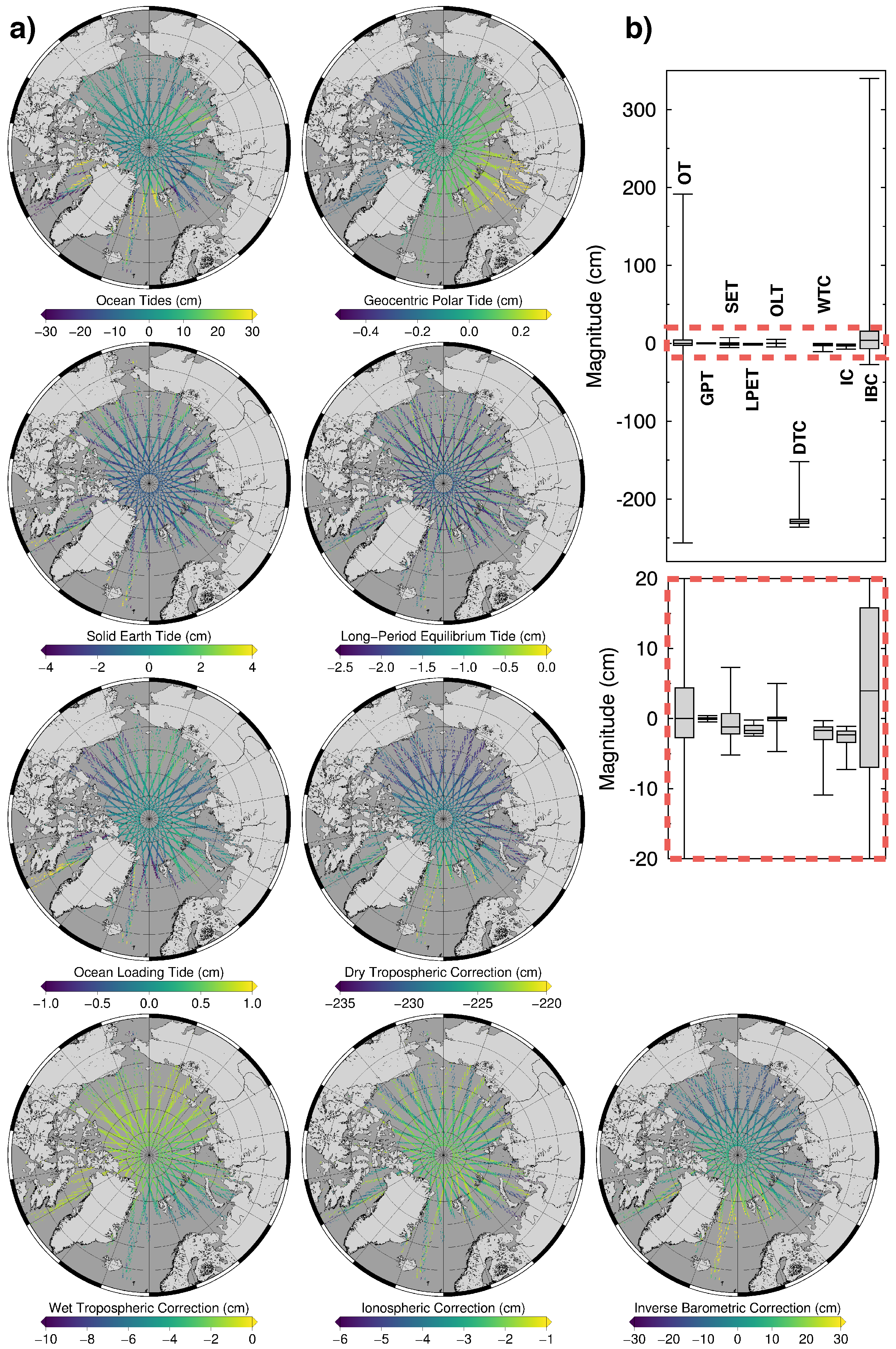
2.1. Geophysical Range Corrections

In the following we describe the geophysical corrections that are used in the CS2 freeboard processing. The corrections are included in the Level-1b sensor raw data files, that are provided by ESA [14] and also contain the geolocated radar echoes that are used to calculate sea-ice freeboard. The corrections can be separated into tidal, atmospheric, and surface corrections. Tidal corrections accommodate for surface elevation changes due to tides. Atmospheric corrections accommodate for the range delay due to the refraction of electromagnetic waves in the atmosphere. Surface corrections accommodate for changes in the atmospheric loading. Figure 1 shows the spatial pattern (a) and dynamic range (b) of each correction for CS2 orbits during the first seven days of March 2015. Below, we refer to the range spanned by the quartiles as the dynamic range, and range spanned by the minimum and maximum value whiskers as the amplitude (the peak-to-peak amplitude).

2.1.1. Ocean Tide (OT)

The Ocean Tide correction removes the effects of tidal forces on the water masses of the Ocean. In order to compute these corrections, the tide model FES2004 is used [15]. The resolution is 0.125 degrees and it covers the entire globe. The dynamic range is approximately 8 cm, but the amplitude is the order of ±450 cm.

2.1.2. Geocentric Polar Tide (GPT)

The Geocentric Polar Tide correction accommodates for small perturbations in the earth’s rotation axis, which cause variations of the centrifugal potential and therefore affects the solid earth and ocean tides. The correction is calculated using daily dynamic files from CNES/SSALTO that contain the pole locations. The dynamic range and amplitude are approximately 0.6 cm, and 2 cm, respectively.

2.1.3. Solid Earth Tide (SET)

The solid earth tide correction accommodates for the deformation of the earth due to tidal forces, in particular by the sun and moon. The correction is computed by a static file, using the Cartwright tables of tidal harmonics [16,17,18]. The dynamic range is about 3 cm with amplitudes on the order of 12 cm.

2.1.4. Long-Period Equilibrium Tide (LPET)

The Long Period Equilibrium Ocean Tide corrects for the tidal forces due to the sun. For this computation, the FES2004 tide model is used [15]. The dynamic range and amplitude are low, about 2 and 4 cm, approximately double of the GPT.

2.1.5. Ocean Loading Tide (OLT)

Due to the ocean tides, water masses in the ocean are shifted. The resulting load changes cause a deformation of the earth’s crust. The ocean loading tide is computed after [18,19], using a static file. For this computation, the FES2004 tide model is used. Dynamic range is about 1 cm, similar to the GPT, but amplitudes span a wider range of approximately 10 cm.

2.1.6. Dry Tropospheric Correction (DTC)

This correction accommodates for the path delay due to the dry gas component of the atmosphere. It is proportional to the sea level pressure and represents the largest of all corrections (on the order of 2.3 m). On the other hand, the dynamic range is low, ∼10 cm, but the amplitude is about 85 cm. The correction is calculated using mean surface pressure grids sourced from Meteo-France via CNES/SSALTO [20], and are based on ECMWF data.

2.1.7. Wet Tropospheric Correction (WTC)

This correction accommodates for the path delay of the returning radar echo caused by the water vapor in the atmosphere. The dynamic range is ∼2 cm and the amplitude is approximately 11 cm. The correction data are taken from Meteo-France via CNES/SSALTO and are based on ECMWF analysis grids [21].

2.1.8. Ionospheric Correction (IC)

This correction accommodates for the path delay due to free electrons in the upper atmosphere. There are two corrections included in the Level-1b product: one is the Bent Model Ionospheric Correction, the other uses the Global Ionospheric Map (GIM). For this study we only use the GIM, since the Bent model is not available for latitudes >82${}^{\circ }$. The GIM correction requires GPS ionospheric data computed every second along the satellite tracks and are obtained from CNES [22]. The dynamic range is similar to WTC (∼3 cm) but the amplitude is smaller (∼6 cm).

2.1.9. Inverse Barometric Correction (IBC) and Dynamic Atmosphere (DAC)

The Inverse Barometric Correction takes into account atmospheric pressure changes which cause a change in the sea surface height. This correction is only applied for the SAR mode, over sea ice and over open ocean. It is derived from the dry tropospheric correction and therefore has a similar spatial pattern [23]. Another geophysical correction contained by the CryoSat-2 Level-1b data is the dynamic atmosphere correction, which basically accounts for the same effect, but is used over open ocean [14]. IBC and DAC should not be applied at the same time. The dynamic range is more than 20 cm, which is even greater than for OT. The amplitude is more than 350 cm. The IBC is calculated from data sourced from Meteo-France via CNES/SSALTO.

2.2. The Impact of Geophysical Corrections on Sea-Ice Freeboard

2.2.1. CryoSat-2 Data Retrieval

The processing of the CS2 freeboard is generally carried out as described in [5]. The geolocated waveforms are provided by ESA in the Level-1b data. A 50% Threshold-First-Maximum retracker [24] is used to obtain ellipsoidal surface elevations. Then, geophysical range corrections (Section 2.1) are added to the range retrieval (L):

$$L_{\mathrm{CORR}}=L+CORR$$

(1)

where $CORR$ is the sum of all applied corrections and $L_{\mathrm{CORR}}$ the corrected range retrieval. Main undulations due to the geoid and the MSS are removed by subtracting the Danish Technical University version 2013 (DTU13) MSS height ($MS{S}_{\mathrm{DTU}13}$ [25]). With a lead detection algorithm, we identify leads along each CS2 orbit and linearly interpolate between these lead elevations [6]. In order to reduce noise due to single-observation-uncertainties [5], the obtained sea-surface height anomaly ($SSHA$) is smoothed over a running 25 km window. The sea-surface height anomaly is then subtracted from ice elevations, yielding freeboard (Fb):

$$\begin{array}{cc}\hfill L_{\mathrm{CORR},\mathrm{MSS}}=& L_{\mathrm{CORR}}-MS{S}_{\mathrm{DTU}13}\hfill \end{array}$$

(2)

$$\begin{array}{cc}\hfill Fb=& L_{\mathrm{CORR},\mathrm{MSS}}-SSHA\hfill \end{array}$$

(3)

This procedure is repeated orbit-wise. For one month, all processed CS2 orbits are averaged on a 25 × 25 km EASE2 grid [26]. In addition to the gridded freeboard, we also compute a gridded lead fraction, which is the fraction of waveforms that are classified as leads to the total number of valid waveforms within a grid cell. For this study, we will use the gridded freeboard and lead fraction retrievals as well as single orbit retrievals.

2.2.2. Experimental Setup

We choose March and November 2015 as our test months for deriving the impact of the geophysical corrections. These months represent the two important states of the Arctic sea-ice season: spring, where sea-ice extent and thickness has reached its maximum, and autumn, after the summer melt and during the freeze-up. We have chosen the year 2015, because the latest CS2 Level-1b data version release by ESA, called Baseline C, was only available for this year at the time of this study. In order to predict the impact of each correction, we switch on every correction individually.

Table 1. List of applied geophysical corrections. For the different runs they are switched on individually. The area fraction A is calculated as the percentage of all valid CS2 freeboard grid cells of a month that are affected by the specific geophysical correction greater than 1 cm. MEAN(|Δ Fb|${}_{\mathrm{A}}$) is the mean of the impact on the freeboard for the grid cells contained in A.

Geophysical Correction	Acronym	March 2015		November 2015
		A (%)	MEAN(|Δ Fb|${}_{\mathrm{A}}$) (cm)	A (%)	MEAN(|Δ Fb|${}_{\mathrm{A}}$) (cm)
Ocean Tide	OT	7.17	4.85	2.33	3.19
Geocentric Polar Tide	GPT	0	–	0	–
Solid Earth Tide	SET	0.05	1.37	0.01	1.53
Long-Period Equilibrium Tide	LPET	0	–	0	–
Ocean Loading Tide	OLT	0.02	1.17	0	–
Dry Tropospheric Correction	DTC	0.27	1.42	0.06	2.23
Wet Tropospheric Correction	WTC	0.06	1.80	0.03	1.24
Ionospheric Correction	IC	0	–	0	–
Inverse Barometric Correction	IBC	2.69	2.22	0.69	2.37

shows the list of geophysical corrections that are applied. Initially, we calculate CS2 freeboard for March and November without applying any geophysical corrections to represent our reference. Therefore, we carry out 10 runs in total for each month. Subtracting the reference run where no corrections have been applied yields the impact of each geophysical correction on sea-ice freeboard ($\Delta Fb$). In order to relate the impact to the freeboard magnitude, we introduce the relative impact ρ, according to the relative error:

$$\rho =\frac{|\Delta Fb|}{F{b}_{{\mathrm{CORR}}_0}}=\frac{|F{b}_{{\mathrm{CORR}}_{\mathrm{i}}}-F{b}_{{\mathrm{CORR}}_0}|}{F{b}_{{\mathrm{CORR}}_0}}$$

(4)

where i is the index for the considered correction, while 0 represents the reference retrieval, where no correction has been applied.

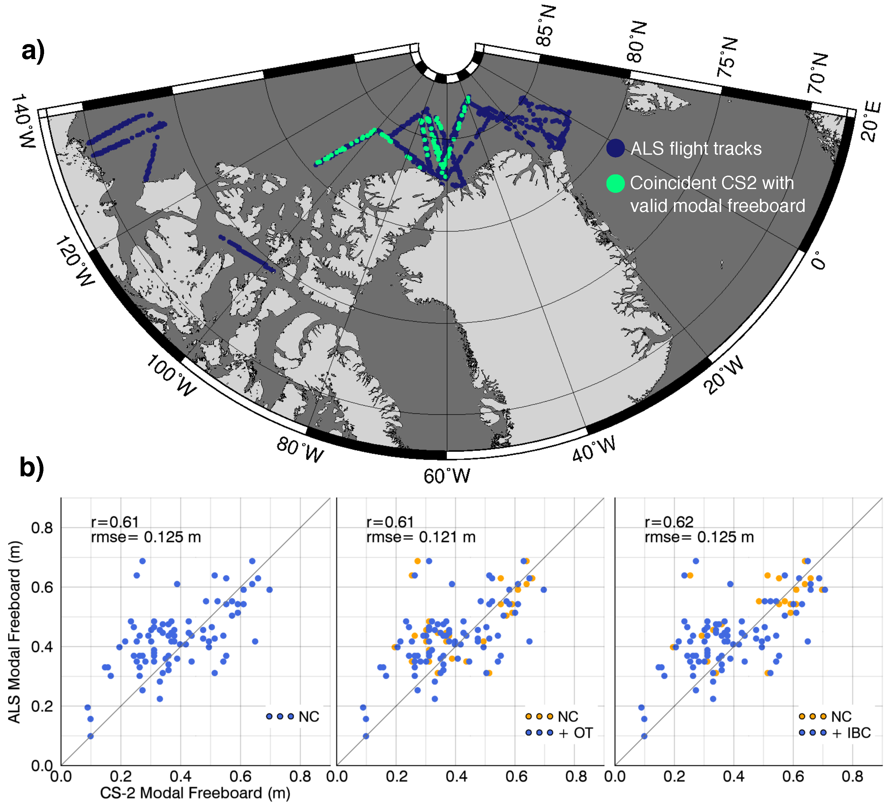
2.3. Airborne Laser Scanner Data and Coincident CryoSat-2 Freeboard

The relative comparison between the different runs provides a measure of the impact but it does not give information regarding the potential improvement to freeboard accuracy by the application of each correction. Therefore, we compare CS2 measurements with coincident airborne laser scanner (ALS) measurements. In the framework of the CS2 Validation Experiment (CryoVEx), several airborne surveys have been carried out from different places in the Western Arctic (Figure 2a). Most of the flight tracks are co-located with CS2 ground tracks and also took place at the same time as the satellite overflight.

For the comparison with ALS, coincident CS2 freeboard is resampled on a 10 × 10 km grid. In order to reduce the effect of deformed sea ice on the freeboard and to reduce noise, we calculate modal CS2 freeboard for the relevant grid cells. The modal value is retrieved by fitting a log-normal function to the freeboard distribution of a grid cell and picking the value at the probability maximum [11]. The CS2 freeboard itself is retrieved according to Section 2.2.1.

ALS provide high-precision and high-resolution measurements: about 300 shots per scan line with a typical spacing of about 30 cm across track and 1 m along track form a digital elevation model (DEM). The ALS Level-1b data contain the ellipsoidal surface elevations that are referenced to the WGS84 ellipsoid. Leads are flagged manually along track. In order to remove the main undulations in the DEM, we initially subtract the DTU13 MSS, as is done in the CS2 processing. After subtracting the DTU13 MSS, lead elevations are interpolated with a spline, which generates the sea-surface anomaly. We use a spline here because we can manually supervise the interpolation and avoid unintended bending. In contrast, as the CS2 processing is carried out automatically, we use a combination of linear interpolation and filtering to retrieve the CS2 sea-surface anomaly. However, the ALS sea-surface anomaly is then subtracted from the DEM, yielding the snow freeboard, the height of the snow surface above the water level. We do not apply any geophysical corrections.

As with the CS2 freeboard, ALS freeboard is resampled on a 10 × 10 km EASE2 grid for direct comparison with the CS2 freeboard. ALS modal freeboard is calculated using a log-normal fit, the same method used to calculate the CS2 modal freeboard.

3. Results

This section presents our case study results and is divided into two parts. The first part is related to the impact of the geophysical corrections on the CS2 freeboard, while the second part shows the results of the comparison with airborne laser data in order to evaluate the corrections regarding potential improvements.

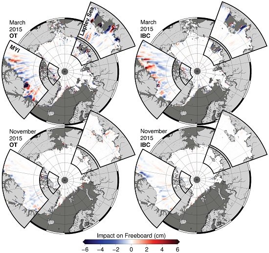
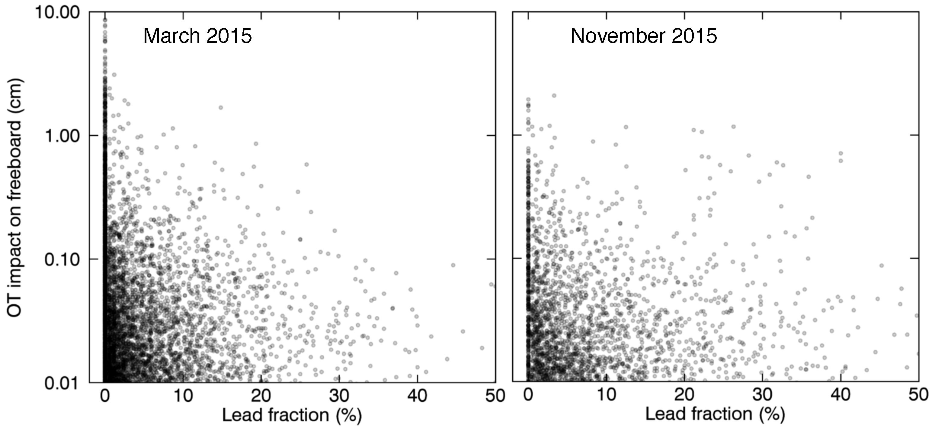
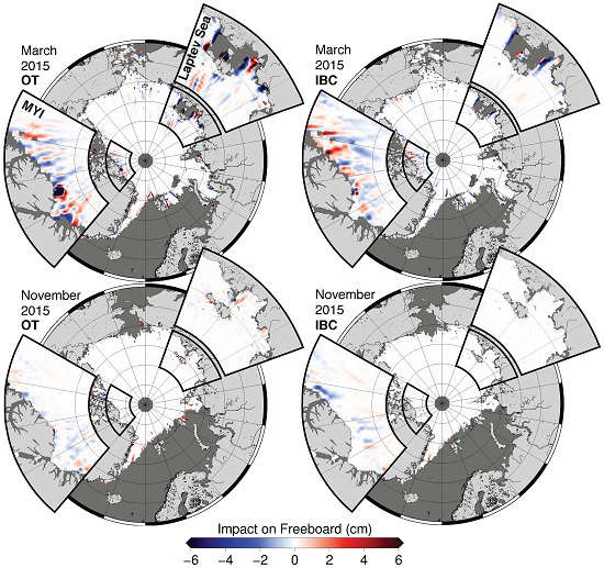
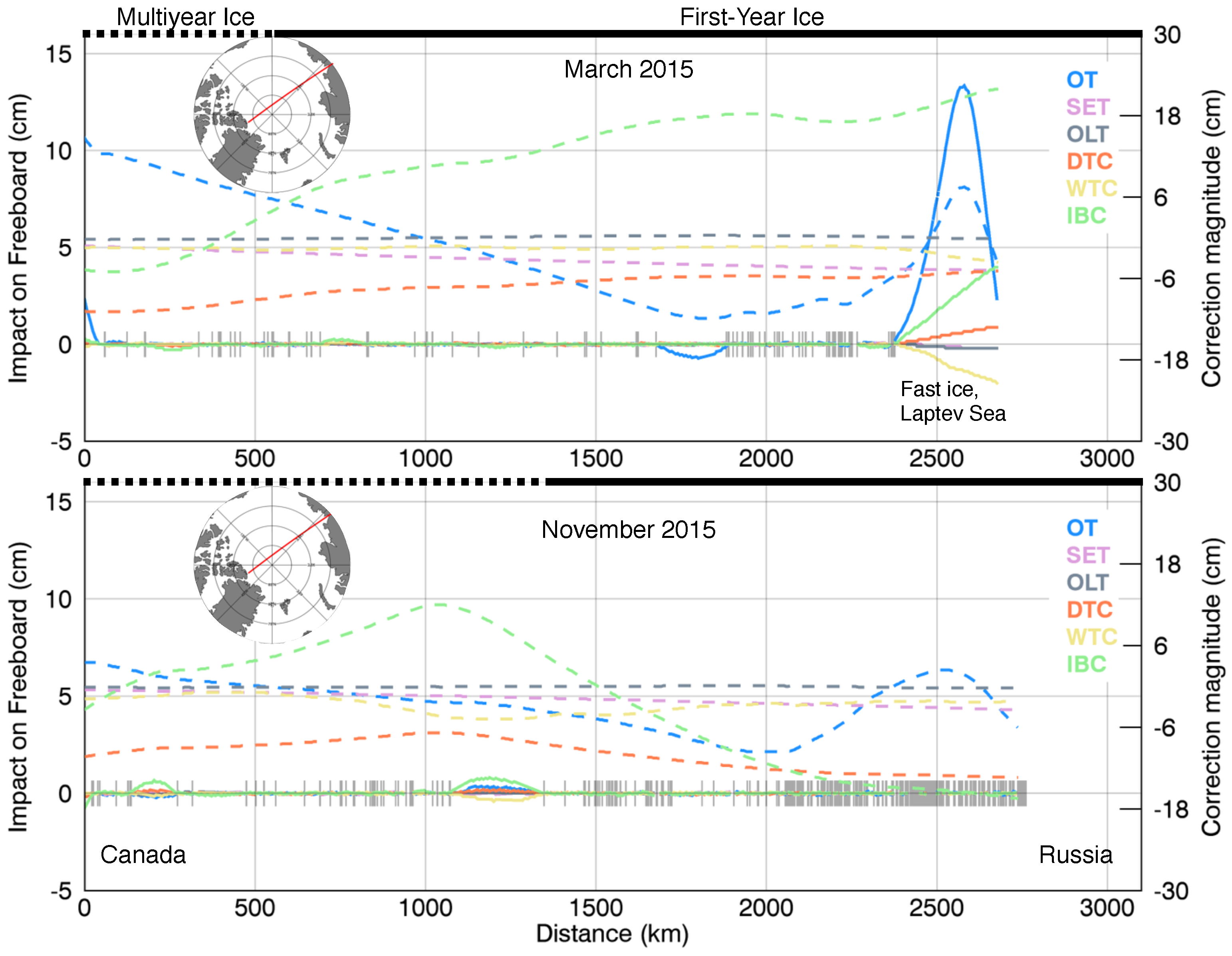
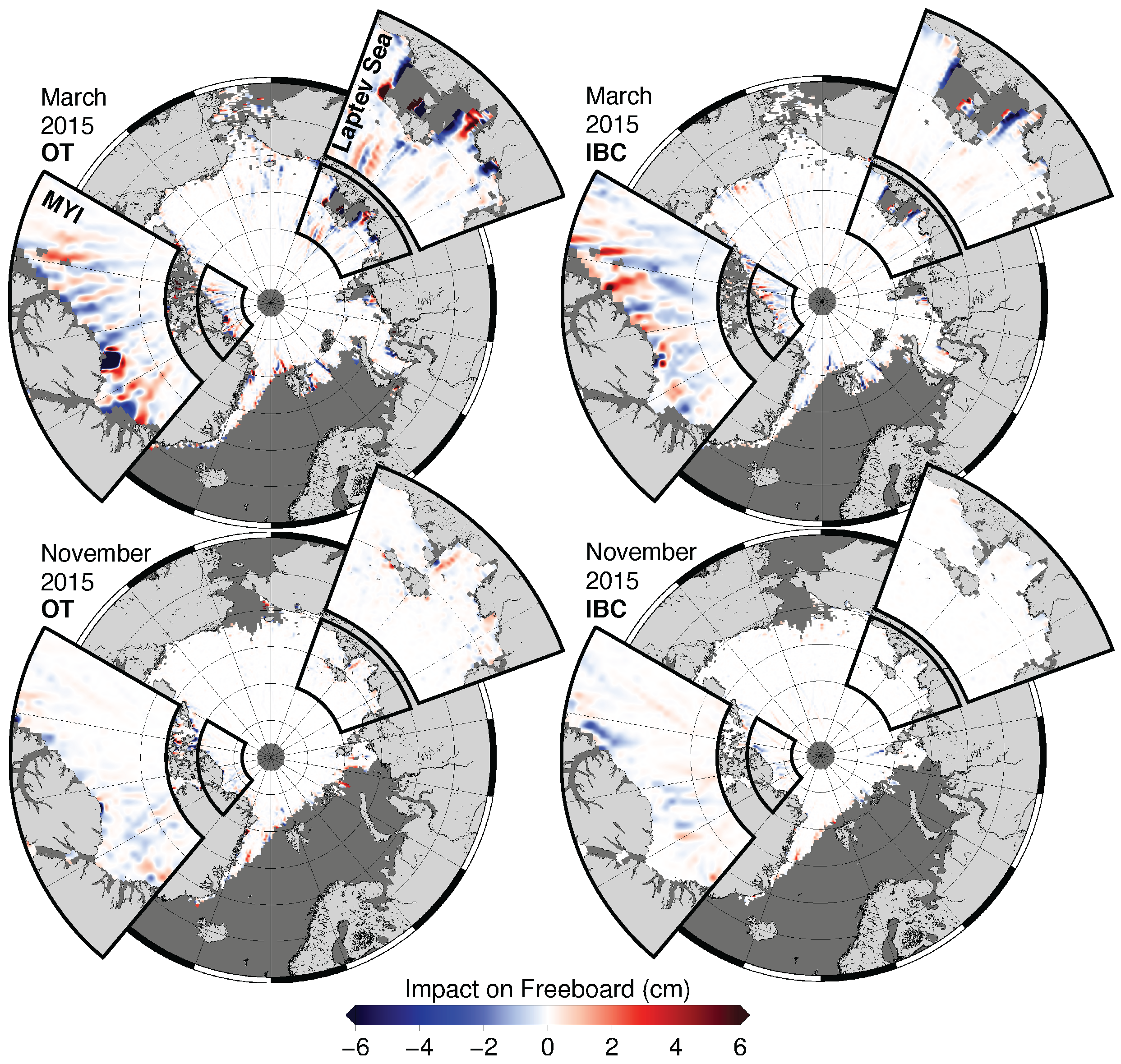
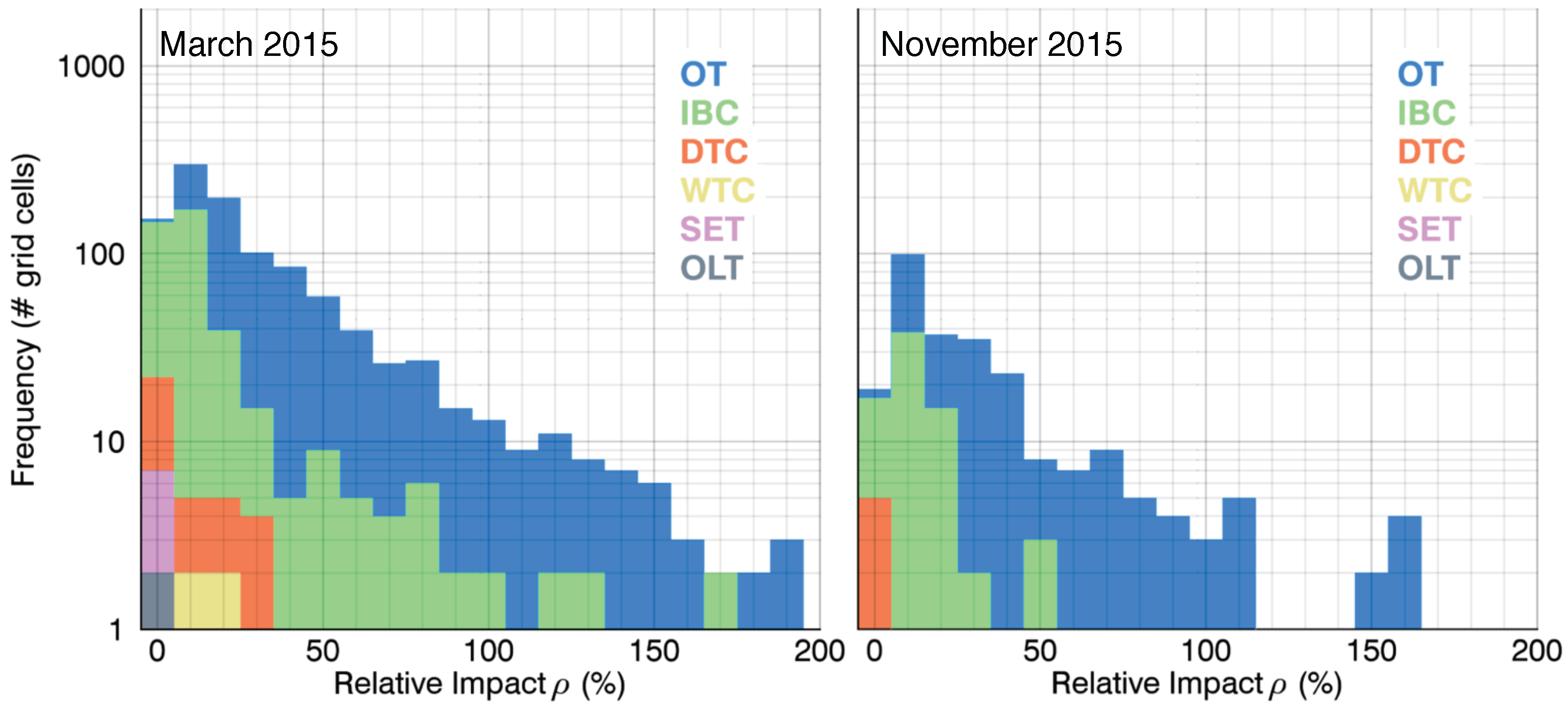
3.1. Assessing the Impact of Geophysical Corrections on Sea-Ice Freeboard

In order to investigate the impact on different scales and product levels, we first subtract the reference retrieval along track from the corrected freeboard retrievals. As a consequence, we have chosen characteristic orbits that cover all relevant ice types: FYI, MYI and landfast ice. We particularly consider two such orbits in March and November 2015. In the second step we subtract gridded monthly means from each other, yielding the impact on the grid scale.

Figure 3 shows the impact on CS2 freeboard for two single orbits in March and November 2015. Both orbit segments start north of Canada in the Lincoln Sea, cross the Arctic Ocean and end in the Laptev Sea. They cover multiyear ice in the Lincoln Sea, first-year ice in the central Arctic, and landfast ice in the Laptev Sea. Generally, we find a higher lead density in November. In March, fewer leads are observed in the multi-year ice zone than in the first-year ice region and no leads are observed in the Laptev Sea where there is extensive landfast ice. Figure 3 only shows 6 of 9 geophysical corrections as we have excluded the impact of GPT, LPET, and IC, since their contributions are not significant (Table 1). In March, the highest impact is caused by OT in the Laptev Sea with a maximum of about 13 cm, followed by IBC, WTC, and DTC. The contributions of OLT and SET are very small and in the range of millimeters. The orbit segment in November shows less impact of geophysical corrections in general and specifically no impact in the Laptev Sea. The major contributors are IBC and WTC with maximums of about 1 cm. We also note the different directions of the correction impacts, meaning that they can also compensate each other partially. In addition, Figure 3 shows the absolute corrections along track. They reveal high variabilities in the range of 25 cm for OT and IBC, while the other corrections only vary within a few cm and also contain only small gradients.

Figure 4 shows the impact of OT and IBC on the gridded freeboard for March and November 2015. It shows a similar pattern as in Figure 3. High impacts can be found mostly at the margins of the ice covered area and particularly in the MYI north of Canada and over fast ice in the Laptev Sea. Affected areas tend to show alternating directions: grid cells of positive impact next to grid cells of negative impact.

In order to quantify the impact in terms of magnitude but also spatially, Table 1 lists the area fraction (A), which is the percentage of affected 25 km grid cells, where the impact is greater than 1 cm, as well as the mean of the impact ($\Delta Fb$) according to A. For both, March and November 2015, the largest A is given by OT, followed by IBC. For the other corrections, A is below 1%. MEAN(|Δ Fb|_A) is dominated by OT for March and November, followed by IBC.

In order to find a relation between A and ρ, Figure 5 shows logarithmic histograms for March and November 2015 with the relative impact on the x axis and the total number of affected grid cells on the logarithmic y axis. The histograms for both months are dominated by the impact of OT and IBC, noting that we generally find higher impacts at a higher frequency in March. GPT, LPET, and IC are not shown here, since they do not show relevant contributions (see Table 1).

3.2. Comparison with Coincident Airborne Laser Scanner Measurements

Figure 2a shows the Western Arctic and the ALS flight tracks during the period 2011–2014 in March and April. We consider CS2 grid cells that contain at least 30 valid single measurements, in order to retrieve a representative modal freeboard. Therefore, only a few grid cells remain for the analysis, specifically the green marked cells in Figure 2a. The scatterplots in Figure 2b reveal the impact of OT and IBC by the relation to the reference run without the corrections. If we consider the ALS modal freeboard as the ground truth, then one should observe improvements in the scatterplot and particularly an increase in the correlation coefficient (r) and a decrease in the root mean square error (rmse). It is obvious that noise clearly dominates and significant improvements due to the corrections cannot be observed, although small changes in r and rmse are acknowledged. Other corrections are not shown here as their impact is even smaller.

4. Discussion

4.1. Assessing the Impact of Geophysical Corrections on Sea-Ice Freeboard

Figure 3 clearly shows that the impact of the geophysical corrections depends on two parameters. The first is the dynamic range, which goes along with the temporal and spatial variation of the geophysical correction. Temporally and spatially constant corrections would not affect the freeboard retrieval in any case. The GPT, LPET, OLT and IC show a dynamic range of only a few cm and neither have substantial gradients along the CS2 orbit segments. Therefore, their impact is very limited (Table 1). The second parameter, which controls the impact, is the lead density. Figure 3 reveals, that the impact clearly correlates with the appearance of leads. For the considered orbit in March 2015, a low lead density coincides with a high gradient in OT, which finally causes the high OT impact. Since the sea-ice freeboard is a relative quantity, calculated by subtracting the instantaneous sea-surface height from the ice surface elevations, the geophysical corrections theoretically do not influence the freeboard. Both the measured sea surface elevation and the ice surface elevation contain the range contribution due to atmospheric perturbations or tidal forces and therefore cancel each other out by subtraction. To be more specific, in the ideal case of a well known instantaneous sea-surface height, geophysical corrections would not have any impact.

However, we have no information about the actual sea-surface height at each ice elevation measurement. It is common practice to interpolate between lead elevations to retrieve a continuous sea-surface height [5,7,8,9,10]. Due to the interpolation, the sea surface height is not tied between two leads or at the end of an orbit segment (Figure 3). Therefore, the correction added to the ice surface elevations is not compensated equally. This effect causes anomalies whose magnitude correlates with the distance to the next lead and the gradient of the correction. At this point it is important to state that the impact is not equal to an error. it simply describes how the correction affects the freeboard. It does not indicate that this leads to a more, or less accurate freeboard.

Figure 3 and Figure 4 show that the impact can be either positive or negative. Hence, the different corrections can partially compensate each other. According to Figure 3, OT has the strongest impact on the freeboard, which goes along with its high dynamic range. The highest impacts in March can be found in lead-free areas like parts of the multiyear ice zone north of Greenland and Canada, and in landfast ice areas such as the Laptev Sea. In coastal areas, the tidal effects are stronger than in the open ocean due to bathymetry and topography. Furthermore, there is additional uncertainty in these regions as tide models generally have problems in such areas [15].

It is obvious that leads are more prominent in November, during the freeze up where sea ice still has many openings. Therefore the impact of geophysical corrections is generally smaller than in March. This is also shown in Figure 4, which reveals the impact on the gridded freeboard. Figure 6 finally shows the direct relation between lead fraction and impact of corrections, taking OT as an example for March and November 2015. Figure 7a shows the lead fraction for March and November 2015 on the grid scale. In March we find very low lead fractions north of Canada and Greenland and no leads in the landfast ice in the Laptev Sea. The lower the lead fraction, the higher the impact. This relation is exponential with a steep increase towards a fraction of 0, where we also find the largest impact values of >1 cm. Nevertheless, the majority of affected grid cells shows an impact of <1 cm.

In order to quantify how each correction finally affects the freeboard, we calculate the relative impact ρ (Equation (4)), which also takes into account the freeboard magnitude. For example, the landfast ice in the Laptev Sea, and in general, first-year ice is thinner, compared to the multiyear ice north of Canada (Figure 7b). Hence, the relative impact is much stronger for such thin-ice regimes. Figure 5 clearly shows how OT and IBC dominate the relative impact. DTC in March 2015 shows the next highest impact with less than 30 grid cells, for which ρ = 10%, and less than 10 for which ρ = 30%–40%. According to OT, on the other hand, there are still more than 10 grid cells which reveal a relative impact of ρ = 100%. Table 1 lists the impacted area fraction and the mean impact of each correction according to the area fraction. It is also clear that GPT, LPET and IC are negligible, mostly due of their low dynamic range. OLT only shows few relevant contributions in March. SET, DTC and WTC also reveal low spatial impact, compared to OT and IBC which dominate the impact of geophysical corrections. However, we find that the major part of the Arctic is not significantly affected by geophysical corrections. Furthermore, according to the affected area, the impact is small compared to other sources of uncertainty, like retracking, mean sea-surface height and snow volume scattering [5]).

4.2. Comparison with Coincident Airborne Laser Scanner Measurements

In order to evaluate potential improvements of the corrections, we compare ALS measurements in the Western Arctic with coincident CS2 freeboard retrievals. Here we assume that the ALS modal freeboard represents the ground truth. Due to the supervised sea surface height and the high precision elevation measurements, the ALS is suitable for satellite altimetry validation. However, Figure 2 reveals that the noise level is too high to find whether or not the correction improves the CS2 freeboard retrieval. Although we observe small increases of the correlation and decrease of rmse, these changes are not significant. One source of the high scattering are the different scales of the footprint. While CS2 has a footprint of approximately 300 × 1650 m, the ALS provides a spatial resolution in the range of centimeters and a swath width in the range of ∼100 m. Another source of discrepancy is the fact that the ALS scans the snow surface, while the CS2 radar penetrates into the snow, potentially scattered by internal layers [11,12]. Although we carefully supervise the ALS modal freeboard, it also contains interpolation errors in the instantaneous sea surface height, despite the potentially more accurate lead detection compared to CS2. Finally, the interpolation errors in the CS2 instantaneous sea surface height also contribute to the uncertainty budget. All these effects contribute to the noise and prevent any further conclusions regarding the improvement through the corrections. On the other hand, the high scattering in Figure 2 gives rise to the assumption, that the CS2 uncertainty sources mentioned above, are much more profound than the contributions from the geophysical corrections.

In the worst case, the geophysical corrections add a bias which is equal to the impact we have computed in this study. By considering the uncertainty budget of CryoSat-2 measurements [5], this bias would be only relevant in lead-free areas like the multiyear ice north of Greenland and Canada or landfast ice. On the other hand, in lead free areas any undulation of the sea level, residuals of the MSS height, including errors in the geoid, can cause substantial interpolation errors which probably superimpose the contribution from the corrections.

4.3. Uncertainties in the Experimental Setup and Advices

Our experimental setup only considered two months in 2015. Additionally, we also tested November 2013 and found similar results, which is not surprising, as the seasonality of lead occurrence and the dynamic ranges of the geophysical corrections does not change substantially. Therefore, we are confident that our findings are representative of other years and months.

This study can provide advice for potential improvements or evaluations of geophysical corrections for sea-ice freeboard or thickness studies. The focus should be set on the ocean tides (OT), especially in the coastal areas, and the inverse barometric effect (IBC). Furthermore, these findings can be also transferred to other altimetry satellites which are used to retrieve sea-ice freeboard, like Envisat, IceSat or upcoming missions like Sentinel-3 or IceSat-2. The retrieved lead fraction differs from sensor to sensor, depending on resolution and sensitivity, and therefore also the impact of geophysical corrections will change, though the principle remains the same.

5. Conclusions

We aimed to evaluate the impact of geophysical corrections on sea-ice freeboard due to atmospheric effects and tidal forces. In this study, we specifically used CryoSat-2 measurements to calculate the impact. However, the findings can be assigned to other altimetry missions over sea ice, since the freeboard processing scheme remains the same. The freeboard is obtained by the subtraction of the instantaneous sea level from the ice surface elevations. Therefore, the freeboard is a relative quantity and ideally, corrections on the range retrieval would not affect the freeboard retrieval. However, the instantaneous sea level is retrieved by interpolation between the elevations of detected leads and with the lack of sea level information in lead-free areas, the geophysical corrections can affect the freeboard retrieval. Hence, the impact of a correction depends on the dynamic range of the correction and the lead fraction. Our findings show that the major sea-ice covered area in the Arctic is not significantly affected by geophysical corrections. Regions with significant impact correlate with low lead fractions or lead-free areas and can be found in the multiyear ice north of Greenland and Canada, as well as over landfast ice, i.e. in the Laptev Sea. During the freeze-up in autumn, the ice cover is characterized by many leads and openings, while they are reduced in spring. Hence, the impact of geophysical corrections is higher in spring when the ice is thickest and generally low in autumn. Among the different corrections, only the ocean tides and the inverse barometric correction show substantial contributions to the impact. These contributions can also compensate each other.

In order to evaluate potential improvements due to the corrections, we compared airborne laser freeboard retrievals in the Western Arctic with coincident CS2 freeboard retrievals, assuming that the airborne retrieved modal freeboard represents the ground truth. There is no evidence for improvements by applying the corrections, since the noise level is too high. This might suggest, that other sources of uncertainty like interpolation errors, snow volume scatter, surface roughness, but also scattering due to the different measurement characteristics, are more substantial sources of uncertainty and therefore mask the effect of the geophysical corrections.

Finally, this study can serve as advice for potential improvements or evaluations of geophysical corrections for sea-ice freeboard or thickness studies. Our findings suggest that the focus should be set on the ocean tides (OT), especially in the coastal areas, and the inverse barometric effect (IBC), while the other corrections are rather negligible.

References

1. Rothrock, D.A.; Yu, Y.; Maykut, G.A. Thinning of the Arctic sea-ice cover. Geophys. Res. Lett. 1999, 26, 3469–3472. [Google Scholar] [CrossRef]
2. Giles, K.A.; Laxon, S.W.; Ridout, A.L. Circumpolar thinning of Arctic sea ice following the 2007 record ice extent minimum. Geophys. Res. Lett. 2008, 35, L22502. [Google Scholar] [CrossRef]
3. Kwok, R.; Cunningham, G.F.; Wensnahan, M.; Rigor, I.; Zwally, H.J.; Yi, D. Thinning and volume loss of the Arctic Ocean sea ice cover: 2003–2008. J. Geophys. Res. 2009, 114. [Google Scholar] [CrossRef]
4. Lindsay, R.; Schweiger, A. Arctic sea ice thickness loss determined using subsurface, aircraft, and satellite observations. Cryosphere 2015, 9, 269–283. [Google Scholar] [CrossRef]
5. Ricker, R.; Hendricks, S.; Helm, V.; Skourup, H.; Davidson, M. Sensitivity of CryoSat-2 Arctic sea-ice freeboard and thickness on radar-waveform interpretation. Cryosphere 2014, 8, 1607–1622. [Google Scholar] [CrossRef] [Green Version]
6. Ricker, R.; Hendricks, S.; Gerdes, R.; Helm, V. Classification of CryoSat-2 radar echoes. In Towards an Interdisciplinary Approach in Earth System Science: Advances of a Helmholtz Graduate Research School; Lohmann, G., Ed.; Springer: Berlin, Germany, 2014. [Google Scholar]
7. Laxon, S.W.; Giles, K.A.; Ridout, A.L.; Wingham, D.J.; Willatt, R.; Cullen, R.; Kwok, R.; Schweiger, A.; Zhang, J.; Haas, C.; et al. CryoSat-2 estimates of Arctic sea ice thickness and volume. Geophys. Res. Lett. 2013, 40, 732–737. [Google Scholar] [CrossRef]
8. Kurtz, N.T.; Galin, N.; Studinger, M. An improved CryoSat-2 sea ice freeboard retrieval algorithm through the use of waveform fitting. Cryosphere 2014, 8, 1217–1237. [Google Scholar] [CrossRef] [Green Version]
9. Kwok, R.; Cunningham, G. Variability of Arctic sea ice thickness and volume from CryoSat-2. Philos. Trans. R. Soc. Lond. A: Math. Phys. Eng. Sci. 2015, 373, 20140157. [Google Scholar] [CrossRef] [PubMed]
10. Tilling, R.L.; Ridout, A.; Shepherd, A.; Wingham, D.J. Increased Arctic sea ice volume after anomalously low melting in 2013. Nat. Geosci. 2015, 8, 643–646. [Google Scholar] [CrossRef]
11. Ricker, R.; Hendricks, S.; Perovich, D.K.; Helm, V.; Gerdes, R. Impact of snow accumulation on CryoSat-2 range retrievals over Arctic sea ice: An observational approach with buoy data. Geophys. Res. Lett. 2015. [Google Scholar] [CrossRef]
12. Kwok, R. Simulated effects of a snow layer on retrieval of CryoSat-2 sea ice freeboard. Geophys. Res. Lett. 2014, 41, 5014–5020. [Google Scholar] [CrossRef]
13. Skourup, H.; Einarsson, I.; Sandberg, L.; Forsberg, R.; Stenseng, L.; Hendricks, S.; Helm, V.; Davidson, M. ESA CryoVEx 2011 airborne campaign for CryoSat-2 calibration and validation. In Proceedings of the 2011 AGU Fall Meeting, San Francisco, CA, USA, 5–9 September 2011.
14. European Space Agency. L1B Products Format Specification; CS-RS-ACS-GS-5106; ESA: Paris, France, 2011. [Google Scholar]
15. Lyard, F.; Lefevre, F.; Letellier, T.; Francis, O. Modelling the global ocean tides: Modern insights from FES2004. Ocean Dyn. 2006, 56, 394–415. [Google Scholar] [CrossRef]
16. Cartwright, D.; Tayler, R. New computations of the tide-generating potential. Geophys. J. R. Astron. Soc. 1971, 23, 45–74. [Google Scholar] [CrossRef]
17. Cartwright, D.; Edden, C. Corrected tables of tidal harmonics. Geophys. J. R. Astron. Soc. 1973, 33, 253–264. [Google Scholar] [CrossRef]
18. Jentzsch, G. Earth tides and ocean tidal loading. In Tidal Phenomena; Springer: Berlin, Germany, 1997; pp. 145–171. [Google Scholar]
19. Farrell, W.E. Deformation of the Earth by surface loads. Rev. Geophys. 1972, 10, 761–797. [Google Scholar] [CrossRef]
20. AVISO+. Available online: http://www.aviso.oceanobs.com/es/data/index.html. (accessed on 21 March 2016).
21. Kruizinga, G.L.H. Validation and Applications of Satellite Radar Altimetry; University of Texas: Austin, TX, USA, 1997. [Google Scholar]
22. Fu, L.L.; Cazenave, A. Satellite Altimetry and Earth Sciences: A Handbook of Techniques and Applications; Academic Press: New York, NY, USA, 2000. [Google Scholar]
23. Wunsch, C.; Stammer, D. Atmospheric loading and the oceanic “inverted barometer” effect. Rev. Geophys. 1997, 35, 79–107. [Google Scholar] [CrossRef]
24. Helm, V.; Humbert, A.; Miller, H. Elevation and elevation change of Greenland and Antarctica derived from CryoSat-2. Cryosphere 2014, 8, 1539–1559. [Google Scholar] [CrossRef] [Green Version]
25. Andersen, O.; Knudsen, P.; Stenseng, L. The DTU13 MSS (Mean Sea Surface) and MDT (Mean Dynamic Topography) from 20 years of satellite altimetry. In Proceeding of the International Association of Geodesy Symposia, Heidelberg, Germany, 13 August 2015.
26. Brodzik, M.J.; Billingsley, B.; Haran, T.; Raup, B.; Savoie, M.H. EASE-Grid 2.0: Incremental but Significant Improvements for Earth-Gridded Data Sets. ISPRS Int. J. Geo-Inf. 2012, 1, 32–45. [Google Scholar] [CrossRef]
Figure 1. (a) The panel shows the ranges and patterns of all considered geophysical corrections. The corrections are retrieved from CryoSat-2 Level-1b orbit files of the first seven days of March 2015. The data are averaged on a 10 × 10 km grid; (b) The Box-plot shows minimum, lower quartile, median, upper quartile, and maximum values of each geophysical correction according to (a). The lower red-dashed box is an enlargement of the upper red-dashed range.
Remotesensing 08 00317 g001
Figure 2. (a) CryoSat-2 validation flight tracks during 2011–2014, where airborne laser scanner (ALS) measurements have been carried out. ALS measurements and co-located CryoSat-2 measurements are averaged on a 10 × 10 km grid. Green dots highlight grid cells where both CryoSat-2 and ALS modal freeboard are valid; (b) Scatterplots of CryoSat-2 modal freeboard against ALS modal freeboard (blue dots) with corresponding correlation coefficient (r) and root mean square error (rmse). The left plot shows CryoSat-2 modal freeboard without any corrections (NC), in the center plot the Ocean Tides (OT) correction is applied, while in the right plot the inverse barometric correction (IBC) is switched on. The orange dots reveal the CryoSat-2 modal freeboard without applying the correction.
Remotesensing 08 00317 g002
Figure 3. The impact of geophysical corrections on the CryoSat-2 freeboard of a single orbit segment (solid lines), which starts in Lincoln Sea north of Canada over multiyear ice and ends over fast ice in the Laptev Sea. The explanation for the acronyms can be found in Table 1. The corresponding dashed lines (right axis) represent the absolute corrections, that are applied. Note, that we increased DTC by 2.2 m to make it visible in this plot (see Figure 1b). The vertical grey lines flag detected leads in the ice cover. The black dashed and solid lines on the top flag the first-year ice and multiyear ice regimes along track.
Remotesensing 08 00317 g003
Figure 4. The maps show the impact of the ocean tides (OT) and inverse barometric correction (IBC) on the CryoSat-2 freeboard regarding the monthly mean freeboard for March and November 2015, averaged on a 25 × 25 km EASE2 grid. Major impact spots are the multiyear ice (MYI) north of Canada, fast ice zones (e.g., Laptev Sea) and the ice edges.
Remotesensing 08 00317 g004
Figure 5. Logarithmic histograms of the relative impact of geophysical corrections on the CryoSat-2 gridded freeboard for March and November 2015. Ocean Tides (OT) and the inverse barometric correction (IBC) clearly dominate. Geocentric Polar Tide (GPT), Long-Period Equilibrium Tide (LPET) and Ionospheric Correction (IC) are not considered because their impact is negligible (see Table 1). The explanation for the acronyms can be found in Table 1.
Remotesensing 08 00317 g005
Figure 6. Relation between the gridded lead fraction and the gridded impact of the ocean tide (OT) on freeboard from March and November 2015. Note the logarithmic y axis.
Remotesensing 08 00317 g006
Figure 7. (a) The lead fraction is calculated as the percentage of CryoSat-2 waveforms that are classified as leads within a 25 × 25 km grid cell. The new formed ice in autumn generally features more leads than in spring. Also note the low lead fraction in the multiyear ice region north of Greenland and within fast ice areas like the Laptev Sea; (b) The sea-ice freeboard is a monthly mean, averaged on a 25 × 25 km EASE2 grid. It clearly shows the contrast between thick multiyear ice north of Greenland and Canada and the thinner first-year ice, respectively new formed ice.
Remotesensing 08 00317 g007