Article

Distinguishing Land Change from Natural Variability and Uncertainty in Central Mexico with MODIS EVI, TRMM Precipitation, and MODIS LST Data

1
Department of Geography and Environment, Rowan University, Glassboro, NJ 08028, USA
2
Graduate School of Geography, Clark University, 950 Main Street, Worcester, MA 01610, USA
3
Clark Labs, Clark University, 950 Main Street, Worcester, MA 01610, USA
4
School of Geographical Sciences and Urban Planning, Arizona State University, COOR 5628, Tempe, AZ 85287-0104, USA
*
Author to whom correspondence should be addressed.
Remote Sens. 2016, 8(6), 478; https://doi.org/10.3390/rs8060478
Submission received: 30 March 2016 / Revised: 26 May 2016 / Accepted: 2 June 2016 / Published: 7 June 2016
(This article belongs to the Special Issue Uncertainties in Remote Sensing)

Abstract

:
Precipitation and temperature enact variable influences on vegetation, impacting the type and condition of land cover, as well as the assessment of change over broad landscapes. Separating the influence of vegetative variability independent and discrete land cover change remains a major challenge to landscape change assessments. The heterogeneous Lerma-Chapala-Santiago watershed of central Mexico exemplifies both natural and anthropogenic forces enacting variability and change on the landscape. This study employed a time series of Enhanced Vegetation Index (EVI) composites from the Moderate Resolution Imaging Spectoradiometer (MODIS) for 2001–2007 and per-pixel multiple linear regressions in order to model changes in EVI as a function of precipitation, temperature, and elevation. Over the seven-year period, 59.1% of the variability in EVI was explained by variability in the independent variables, with highest model performance among changing and heterogeneous land cover types, while intact forest cover demonstrated the greatest resistance to changes in temperature and precipitation. Model results were compared to an independent change uncertainty assessment, and selected regional samples of change confusion and natural variability give insight to common problems afflicting land change analyses.

Graphical Abstract

1. Introduction

While the influence on vegetative vigor of climatic variables such as precipitation and temperature relates to the type and condition of land cover, the isolation of this variability independent of discrete land cover change is a major challenge of the geographic information science, remote sensing, and land change science communities. In the heterogeneous and rapidly changing Lerma-Chapala-Santiago watershed of Mexico [1,2,3,4], natural and anthropogenic factors, including droughts, the El Niño Southern Oscillation, agricultural expansion, and forest loss enact changes in the remotely sensed detection of vegetative vigor. This study assessed variability using a time series of Enhanced Vegetation Index (EVI) composites from the Moderate Resolution Imaging Spectoradiometer (MODIS) for 2001–2007 and per-pixel multiple linear regressions in order to model changes in EVI as a function of precipitation, temperature, and elevation.
The natural variability of vegetation vigor due to the individual and compound effects of temperature and precipitation has been investigated in numerous geographical contexts, primarily through the use of ground-based observation stations or data from the Advanced Very High Resolution Radiometer (AVHRR) [5]. The need for both inter- and intra-annual analyses for both short-term assessments and long term monitoring and prediction has been affirmed by many researchers, but systematic data errors and coarse global datasets have hindered applicability of studies to local and regional contexts [6,7,8]. Still, the direct and immediate relationship of increased precipitation to positive changes in vegetative vigor has been established through the use of remotely sensed data in mid-latitude semi-arid environments, such as those in central Mexico [9,10]. Because natural variability may diminish or exaggerate the ability of researchers to monitor discrete changes in land cover with satellite-derived image products [11], it is important to consider the climatic conditions concurrent with land change analyses [12] to avoid both errors of omission and commission in land cover change detection and quantification.

1.1. Vegetation Indices and Vegetative Vigor

Improving the ability to measure the quantity and condition of vegetation from remote sensing instruments has been an intensive endeavor for more than 40 years. Early efforts by ecological pioneers such as Jordan [13] and Sellers [14] to relate the quality of light reaching the forest floor to metrics like leaf area index, have been refined into vegetative indices (e.g., the work of Tucker [15]), which attempts to maximize the difference between reflected variables to generate metrics of vegetative vigor. The investigation of phenological variability, including changes to the timing and duration of growing seasons, has been facilitated through the increased availability of continuous temporal datasets, such as AVHRR [16,17] and MODIS [18]. Previous studies have indicated changes in the length and onset of growing seasons around the world, which have been ascribed to interannual variability or long-term climatic trends [17,19]. These changing intra-annual patterns are ascribable to both climactic variability and changing land uses [18,19], and regions experiencing these changes are highly susceptible to misidentifications of land change [20].
The Normalized Difference Vegetation Index (NDVI) has been the most widely used vegetation index, and its broad utility across different land covers and remote sensing instruments has led to tremendous gains in the understanding of regional and global land cover [21,22]. Over tropical and subtropical regions, the NDVI ratio, using satellite image bands in the red and near-infrared ranges, is subject to saturation in cases of high vegetative vigor and sensitivity to atmospheric conditions [22]. Numerous efforts to quantify the relationship between reflected radiation and ecological variables such as leaf-area index and vegetation cover [5,14] have led to improvements upon the NDVI [22]. The Enhanced Vegetation Index (EVI) (designed to minimize haze effects on red reflectance and expand radiometric sensitivity to varying amounts of vegetation, by incorporating blue band and correction constant values) has been systematically evaluated and compared to NDVI in tropical and subtropical environments, and EVI has proven robust to saturation in regions of dense vegetation, while remaining sensitive to variations in canopy cover [23,24]. Several studies have compared the effectiveness of NDVI and EVI in tropical [25] and semi-arid environments [26], noting the close relationship between the two indices. In a study of the effect of sub-pixel mixing of land cover on the values of vegetation indices, Liu and Kafatos [27] found that EVI varied less than NDVI in areas of mixed land cover, making it especially suitable in heterogeneous landscapes. Therefore, the MODIS monthly 1-kilometer EVI composite product was chosen to represent the vegetative vigor of land cover in relation to climate variables of temperature and precipitation.

1.2. Linear Modeling in Time Series Analysis

Linear modeling, in which predictor equations are calculated based on the correlations of ordinary least squares regression, has proven useful in identifying and quantifying the relationships among time series of bioclimatic variables [28]. The use of linear modeling in the context of time series analysis identifies the relationship among temporal sequences of imagery, rather than individual images. Rather than a single slope and intercept to define the terms of the relationship, the relationship of the dependent variable to the independent variables is calculated on a per-pixel basis.
The relationship of temperature and precipitation with variation in vegetation indices has been evaluated using AVHRR [6,29] and ground-based data [12]. In almost every global ecosystem, there is a positive relationship between increased precipitation and increased vegetation index values, especially in water-stressed regions [6,30,31]. Generally, in both semi-arid and sub-tropical regions, a negative relationship between temperature and EVI indicates vegetation vigor is limited by water availability and especially soil moisture [7,8,32]. In the investigation of time series relationships, a change in an independent variable may occur concurrently with a change in the dependent variable. Alternately, a lagged effect implies that a change in an independent variable may precede a change in the dependent variable or that changes in the dependent variable were ascribable to the compound effects of the preceding changes in the independent variables. Wang and colleagues have demonstrated that while there are lagged effects of precipitation and temperature upon vegetation variation, the highest correlation occurred within one or two biweekly periods, or approximately one month [31]. Further, Braswell and colleagues note that there are both significant instantaneous and lagged relationships among vegetation and temperature and that these vary across ecosystems [7]. While lagged links between EVI and climate variables may represent subtle ongoing processes of change [33], they are not effective for the identification of discrete categorical change due to the longer timelines in which these changes occur. As the impacts of precipitation on the natural and rain fed agricultural landscapes of this region would have a quicker impact than the temporal resolution of the data, this study addresses the instantaneous changes in temperature and precipitation that occur concurrently with changes in EVI in order to relate the changes in vegetative vigor to the identification of discrete change in categorical land cover assessments.

1.3. Study Area

This research was conducted in the Lerma-Chapala-Santiago watershed (Figure 1) of central Mexico (19–23.5°N, 99–105.5°W), on Mexico’s Central Mesa, bordered to the south by the Transverse Neovolcanic Mountain Range [34]. Encompassing nearly 136,000 square kilometers, the watershed spans more than 4000 meters in elevation, including the drainages of the Lerma River (Río Lerma) and the Santiago River (Río Grande de Santiago) [35].
This region includes a wide variety of climatic zones and natural vegetation types, due to its diverse topography and geomorphology [34]: semi-arid, dry-steppe, humid sub-tropical, pine-oak forests, and others. As a region situated within the tropics, cyclical patterns of natural variability, such as the El Niño Southern Oscillation, have a direct and immediate effect on precipitation regimes [36]. The phase of El Niño brings cooler temperatures and increased precipitation, while the complementary phase of La Niña is associated with dryer, hotter conditions [36]. During this study, a minor La Niña pattern was identified in 2000–2001 and 2007, and an El Niño pattern has been identified in the winters of 2002–2003, 2004–2005, and 2006–2007. Additionally, the region is subject to the potential influence of both Atlantic (Caribbean) and Pacific hurricanes, though its elevation and relative topography limit the influence of these forces largely to changes in precipitation [36,37].
Patterns indicating widespread drying phenomena have been noted across southwestern North America [38], and there are indications of a major drought in Mexico in the early twenty-first century [39]. Across central Mexico, there are numerous unprotected water bodies that qualify as threatened wetland ecosystems under international conventions [40], and large lakes in this study area, including Chapala and Cuitzeo, have seen volumes decline at an unprecedented rate over recent decades [35,41]. Drought events have a major impact on the Mexican agricultural sector and the communities who depend on it [42,43], and the linear patterns of increased drying and decreased precipitation are shaping a variety of industries [44].
The natural heterogeneity of the region is exemplified by a wide variety of plant species. There are more than 40 species and recognized variations of pine trees in the Republic of Mexico [45], and the Transvolcanic range and Central Mesa are recognized as centers of pine species diversity in Mexico [46]. The Monarch Butterfly Biosphere Reserve, on the edge of the watershed near the borders of the states of Michoacán and Mexico, represents a unique realized niche critical to the annual cycle of the global population of the species [47].
The broad range of natural variation in land cover types and the apparent fluctuation in vegetation vigor across the region is exacerbated by human activity. In addition to extensive heterogeneity in its natural cover, the Lerma-Chapala-Santiago watershed includes several major urban centers, including the cities of Guadalajara (1.7 million inhabitants), Toluca (~750,000 inhabitants), Queretaro (~730,000 inhabitants), Aguascalientes (~700,000 inhabitants), Morelia (~640,000 inhabitants), and Guanajuato (~480,000 inhabitants) (INEGI, 2005). With many regional urban centers within the watershed and Mexico City just beyond its limits, the expansion of the built environment exerts a strong and constant pressure on natural land covers [48,49] and water resources [35,50,51]. Processes of urbanization, extensive and intensive agriculture, timber harvesting, and mining fragment the landscape, creating a motley patchwork of human and natural land covers across most of the watershed [3,52,53]. Additionally, this agriculturally-intensive region has seen a trend toward the consolidation of smallholders’ plots into more commercial and mechanized agricultural systems [54,55]. The watershed is a major producer of corn for the region and the country, and increased investment in tequila production has led to the conversion of fields to agave cultivation in the western state of Jalisco [56,57].
Many landscapes in the region comprise a heterogeneous mixture of multiple covers. In the classification scheme of the International Geosphere-Biosphere Program Data and Information System (IGBP-DIS) DISCover land cover product, a thematic class of “Cropland/Natural Vegetation Mosaic” was included to accommodate cover types that did not represent pure endmembers of either natural or anthropogenic land covers [58,59]. This “Mosaic” cover is especially appropriate in the diverse Lerma-Chapala-Santiago watershed as a buffer class between cropland and natural land covers, as well as serving as an indicator of forest fragmentation or harvesting [58,60].

2. Materials and Methods

Data for this project included vegetation index and land surface temperature products from MODIS, average daily precipitation from TRMM, a DEM from SRTM, and maps of land cover persistence and change [1]. Methods explicated below included the extraction of summary statistics from the time series of dependent and independent variables and a multiple linear regression, performed over the seven-year series and each annual subseries independently (summarized patterns of EVI, precipitation, and temperature shown in Figure 2). Results of the regression model were compared to a previous land cover and uncertainty analysis to explain the effect of variability upon land change error and confusion [1].

2.1. Indices of Vegetative Vigor

Enhanced Vegetation Index (EVI) image composites produced by MODIS product MOD13A3 were used for this study. This product is a monthly maximum value composite of observations from the MODIS instrument on the Terra platform, with a spatial resolution of 1 km per pixel and continuous coverage over the period of study, 2001–2007. As this imagery has undergone geometric correction and compositing by the producers to accommodate periods of impaired observations [61], no further correction was performed in this study.

2.2. Temperature, Precipitation and Elevation Data

Land surface temperature data were derived from the MODIS Terra product MOD11C3, which are distributed as monthly composites of 0.05 degrees per pixel. Data units were transformed from Kelvin to degrees Celsius to maximize interpretability of the results, as negative temperature values were not present in the sample.
Precipitation data were derived from the Tropical Rainfall Measuring Mission product 3B43, which are distributed as monthly composites of average hourly precipitation at 0.25° per pixel [62]. Precipitation data values were rescaled from mm/hour to mm/day to maximize interpretability of the results.
To account for the effects of elevation upon temperature and precipitation [63,64], a digital elevation model (DEM) from the Shuttle Radar Topography Mission was included in the regression analysis as a constant. A series of identical SRTM images was used in the regression to mimic a temporal sequence of the static variable. A random factor of less than one meter was added to all SRTM images to avoid the calculation of a singular correlation matrix among this series.
To ensure geometric compatibility with the series of vegetation indices, all temperature, precipitation, and elevation images were geometrically reprojected and downsampled to 1 km per pixel resolution in the sinusoidal references system using a bilinear calculation [65].

2.3. Land Cover Dynamics

Maps of eight natural and anthropogenic land cover categories for 2001 and 2007 were crosstabulated to identify regions of persistent and changing land cover over the seven-year period [1] (Figure 3). Land cover classes were based on a systematic roadside survey of the Lerma-Chapala-Santiago during January and July 2007 and included the following thematic categories: forest; shrub; grass; sparse vegetation; built (including urban and rural settlements); crop (including mechanized and smallholder agriculture); and mosaic (defined by a sub-pixel mixture of cropland and natural vegetation). Land cover maps were generated for 2001 and 2007 using a combined pseudo-invariant calibration database and the Mahalanobis distance classifier in the Idrisi Taiga software package [1]. Overall map accuracy for the both maps was approximately 90%.
Regions of changing and persistent land cover were further refined using the Confusion Index metric derived from soft-classified Mahalanobis typicality images for both dates [1]. The Confusion Index (CI) quantifies the potential for error in land change assessments based upon the uncertainty inherent to each map used for the change assessment, identifying potential cases in which classification error in one or both maps may contribute to the misidentification of landscape change. CI values range from 0 to 1, in which low values represent a low likelihood of spurious change assessments and higher values indicate apparent change (or persistence) in the imagery may not match true landscape dynamics. For this study, land cover persistence and change assessments were thresholded at a level below 0.3, based on the results of a sensitivity analysis, to isolate the transitions in which there was the highest confidence.

2.4. Multiple Linear Regression

Multiple linear regression was used to model the series of monthly EVI composites as a dependent variable against the independent variables of precipitation and temperature. Through the use of the Earth Trends Modeler of the Idrisi Taiga software package [66], per-pixel slope and intercept terms were calculated as well as a spatially-explicit coefficient of determination for the modeled relationship. Models were generated using the seven-year series of 84 months as well seven independent annual series of 12 months/year. Model results of the seven-year series (R2) are shown in Figure 4.

2.5. Statistics of Variability and Model Performance

Summary statistics of the average monthly of EVI, temperature, and precipitation and the annual variability of each of these variables were calculated over the entire study area. The mean and standard deviation of the monthly spatial averages was calculated to indicate the temporal variability of each variable for each location through time on an annual basis. Additionally, the spatial population standard deviation was calculated from the annual mean EVI images to illustrate the variability across space.
The spatially-explicit model equation terms and the coefficient of determination were averaged over the scale of the entire watershed as well as the isolated regions of persistent and changing land cover, for the seven-year series and the annual series relationships.

2.6. Selected Sample Regions

Four selected sample regions were isolated based on model performance and Confusion Index (CI) values to illustrate potential cases in which land cover change and persistence may or may not be conflated with natural variability. Regions were selected quantitatively through the logical intersection of very low (<0.4) and very high (>0.7) CI, which ranged from 0 to 1, and model R2 values, which ranged from 0 to 0.84. Areas with low CI comprised 22.0% of the landscape, while areas with high CI comprised 49.0% of the landscape. Areas with low R2 values comprised 7.7% of the landscape and high R2 values comprised 15.3% of the landscape. The intersection yielded the four zones from which samples were selected, with their proportional area of the entire Lerma-Chapala-Santiago watershed: low R2 and low CI, 2.2%; low R2 and high CI, 3.8%; high R2 and low CI, 3.6%; high R2 and high CI, 6.7%. A region of approximately 21.4 square kilometers (corresponding to 25 1-kilometer MODIS pixels or 100 500-m pixels) was selected to represent each sample. Land cover composition in 2001, 2007, Confusion Index, Model R2, Average EVI, and Annual EVI profiles for 2001 and 2007 were extracted for each sample (illustrated in Figure 5).

3. Results

3.1. Average Characteristics of Dependent and Independent Variables by Series

Over the seven-year period, the average EVI value across the entire Lerma-Chapala-Santiago watershed was 0.270, with a temporal standard deviation of 0.100 and a spatial standard deviation of 0.408, demonstrating the range of variability of this landscape. Annual average EVI values ranged from a low of 0.255 in 2001 to a high of 0.284 in 2004. The temporal standard deviation of the seven-year series was 0.100, which varied on an annual basis from a low of 0.096 in 2006 to a high of 0.105 in 2007. The spatial standard deviation calculated of the averages of the seven-year series was 0.058, which varied in the annual series from 0.59 (2006) to 0.062 (2004 and 2005).
Average daily precipitation over the entire series was 1.793 mm/day, with a standard deviation of 2.158 mm/day. On an annual basis, average daily precipitation ranged from a high of 2.579 mm/day in 2004 to a low of 0.769 mm/day in 2005. Average daytime temperature over the seven-year series was 30.357 degrees C, with a standard deviation of 5.980 degrees C. Annually, average daily temperature ranged from a high of 31.440 degrees C in 2001 to a low of 28.457 degrees C in 2004. In the SRTM DEM, the elevation of the Lerma-Chapala-Santiago watershed ranges from 4360 m to sea level, with an average elevation of 1903.9 m. Table 1 details summary statistics of EVI, precipitation, and temperature, and the profiles of each of these variables is illustrated in Figure 2.

3.2. Average Characteristics of Dependent and Independent Series by Land Cover Type and Dynamics

Average EVI values across the sample set of persistent land cover type varied widely. Water, with little vegetative response, had a mean EVI value of 0.022 across the seven-year series. The highest mean EVI value was in the forest class, with 0.304, and the lowest mean EVI was in the built class, at 0.151. Agricultural classes of crop and mosaic had average EVI values of 0.296 and 0.298, respectively.
Precipitation falling on each land cover type varied accordingly with its distribution across the watershed, ranging from a high of 1.903 mm/day for the mosaic class to a low of 1.395 mm/day for the grass class. Similarly, average daytime temperature ranged from lows of 22.7 degrees C across the water cover and 25.5 degrees C across the forest cover to 34.4 across sparsely vegetated land cover.
When averaged over each land cover class, EVI generally exhibited a positive relationship to elevation (R2 = 0.41), supported by the high average EVI and high elevation of the forest class. Average temperature and elevation over each land cover showed a weak negative correlation (R2 = 0.03), and there was no demonstrable relationship between precipitation and elevation over the averaged extent of each land cover.
For all persistent land covers, the mean EVI for the seven-year series was 0.281, with an average precipitation of 1.793 mm/day and temperature of 30.3 degrees C. For any land cover that confidently experienced a categorical shift [1], the mean EVI for the seven-year series was 0.260, with average precipitation of 1.787 mm/day and temperature of 30.9 degrees C. Table 2 details summary statistics of average EVI, temperature, and precipitation by land cover type and dynamic over the seven-year series.

3.3. Model Performance by Series

The model indicated that 59.1% of the variability in the dependent variable (EVI) was explained by precipitation, temperature, and elevation over the seven-year series from 2001 to 2007 (Figure 4). On an annual basis, EVI exhibited a varying relationship with the independent variables. From 2001 to 2004, model performance across the watershed was high, with 71.5% (2001) to 79.1% (2002) of the variability in EVI explained by precipitation, temperature, and elevation. In 2005 the model relationship decreased, with only 52.5% of the variability in EVI explained by independent variables. In 2006, model performance was highest among all years studied (R2 = 0.798), and in 2007, model performance decreased slightly, explaining only 68.1% of the variability in EVI. Table 3 summarizes the annual and series model performances, as well as the slope and intercept coefficients for each model.

3.4. Model Performance by Land Cover Type and Dynamics

Across the seven-year series, the average performance of the per-pixel multiple linear regression varied widely by land cover type. Table 4 summarizes the performance of the seven-year per-pixel multiple linear regression model by land cover type and dynamics. In a sample of confidently persistent land covers, on a per-class basis, from 45.9% to 68.0% of the variability in EVI values was explained by independent variables temperature, precipitation, and elevation. Persistent forested landscapes showed the lowest modeled relationship, with only 45.9% of the variability in EVI values explained by the independent variables. The highest model performance was in the mosaic class, explaining 68.0% of the variability in EVI values. Water was excluded from aggregations of land cover, due to the very low relationship among its vegetative vigor (ascribable mostly to changing water levels and eutrophication), temperature, and precipitation. For any pixel that experienced a categorical change in land cover type over the seven-year period, 64.5% of the variability in EVI values was explained by the independent variables. Of the sample of persistent land-based classes, the model explained 56.9% of the variability in EVI values.

3.5. Model Performance, Confusion, and Land Change in Selected Samples

Four sample regions were selected to evaluate the cases in which high and low Confusion Index values intersected with high and low coefficients of determination in the seven-year model (Figure 5).
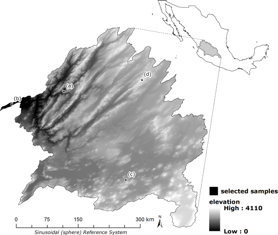
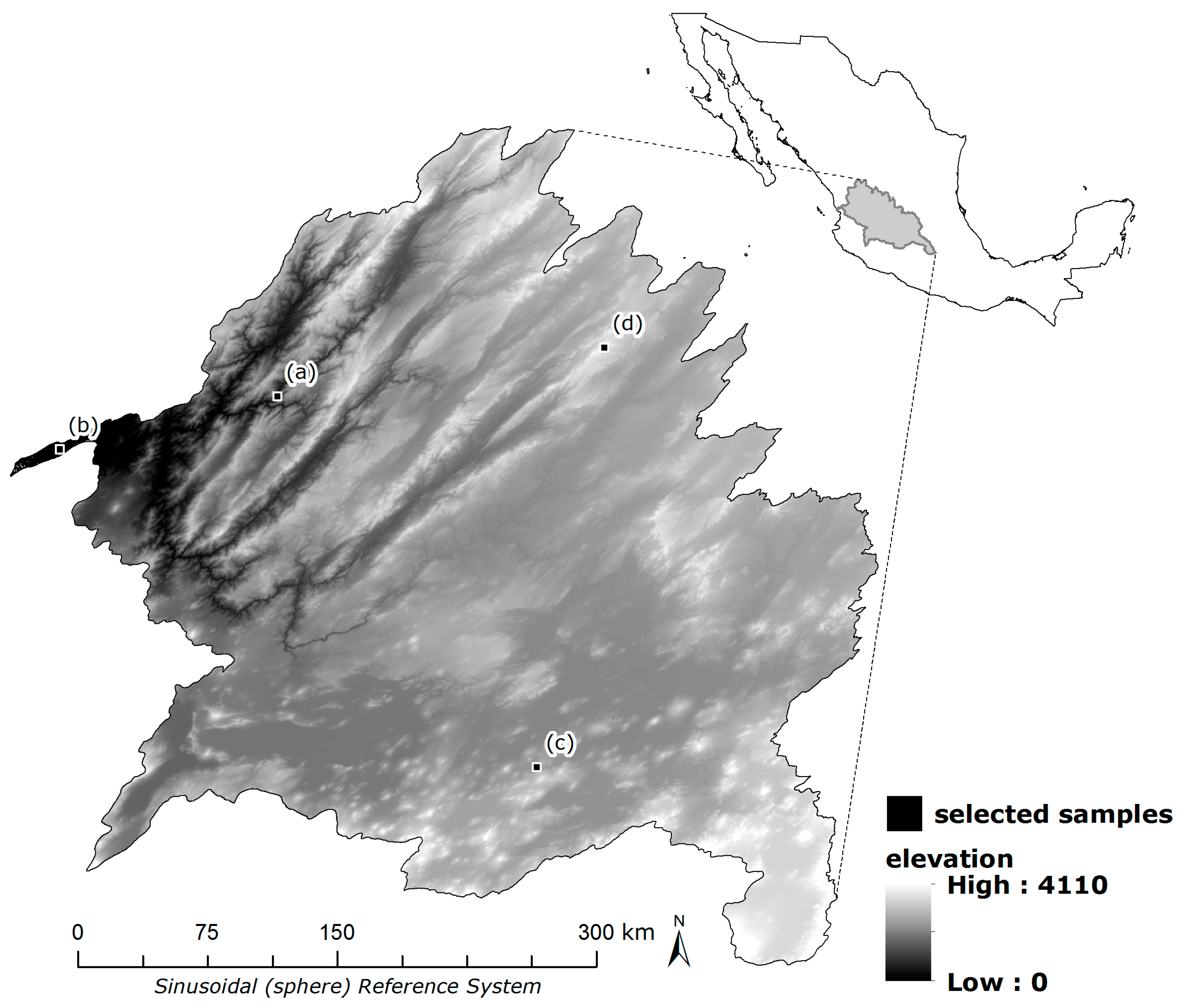
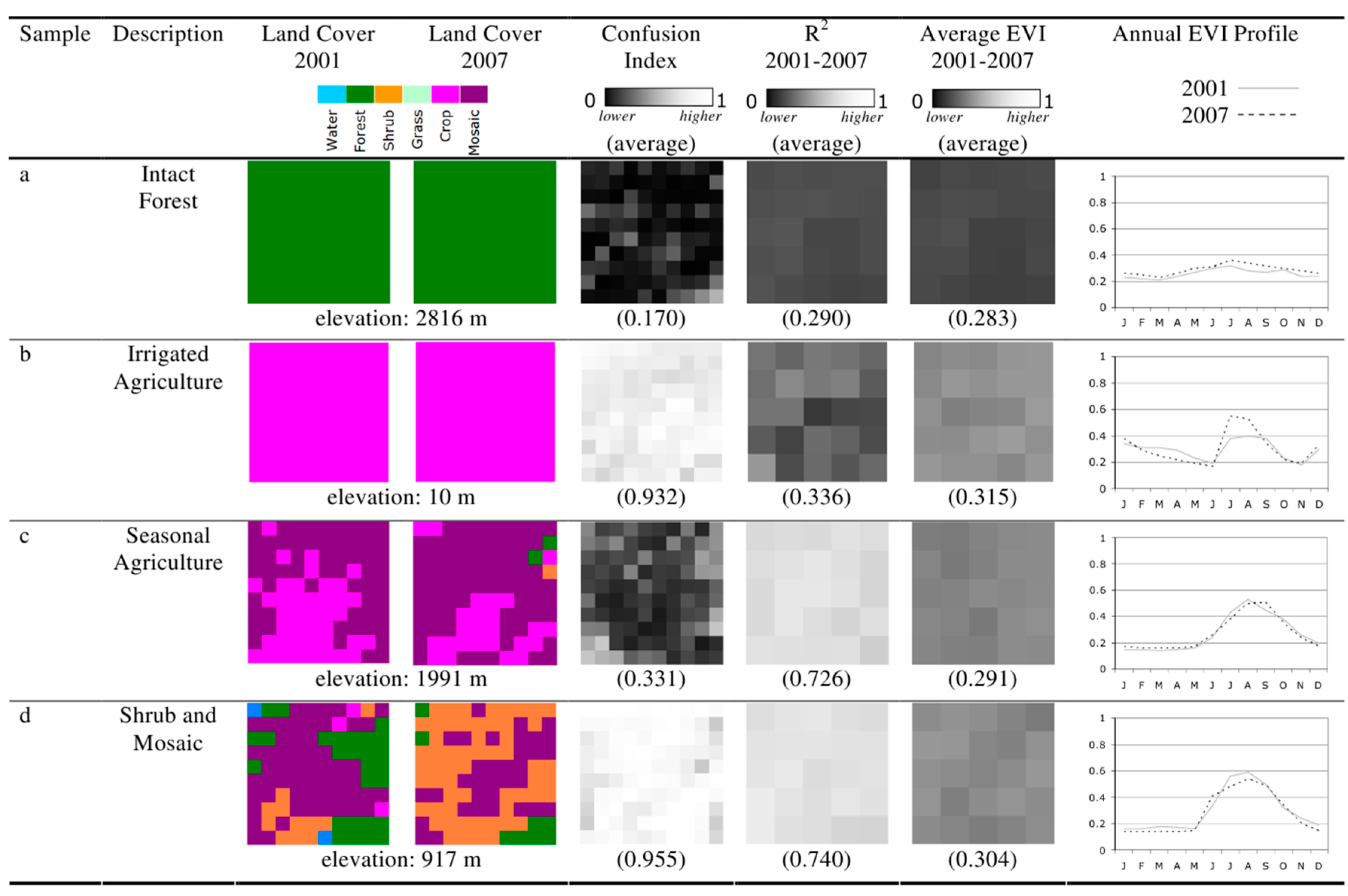
  • The first region (Figure 5a), a parcel of intact forest on the border of the states of Zacatecas and Aguascalientes, is representative of poor model performance with low potential for spurious change assessments and was selected for its low CI (0.170) and low R2 (0.290). In the land cover assessments for both the 2001 and 2007, 100% of the pixels were classified as forest, and the average EVI value over all years was 0.283. Examination of the EVI profiles for 2001 and 2007 indicated similar pattern variability in values over each year.
  • The second region (Figure 5b), a stretch of irrigated agriculture in the state of Nayarit, at the very end of the Rio Grande de Santiago delta, is representative of poor model performance with high potential for spurious change assessments and was selected for its high CI (0.932) and low R2 (0.336). In both 2001 and 2007 land cover assessments, 100% of the pixels were classified as agriculture, with an average EVI value of 0.315 for this period. Examination of the EVI profiles for 2001 and 2007 indicated increased vegetative vigor during the growing seasons of July, August, and September in 2007 compared to 2001.
  • The third region (Figure 5c), a stretch of seasonal agriculture in the northern portion of the state of Michoacán near the border of Guanajuato, is representative of high model performance with low potential for spurious change assessments and was selected for its low CI (0.331) and high R2 (0.726). In the 2001 land cover map, 49% of the pixels were classified as cropland, and 51% as mosaic cover. In the 2007 assessment, mosaic cover increased to 72% of the classified pixels, cropland decreased to 25%, and forest and shrub covered 1% and 2% of the pixels in the parcel, respectively. The average EVI value for this sample was 0.291 for this period. EVI profiles for 2001 and 2007 demonstrated a very similar pattern for both years.
  • The fourth region (Figure 5d) is a heterogeneous plot of shrub, forest, and mosaic cover in the northern region of the state of Jalisco, in an area along a small river basin, where logging is prevalent. This region demonstrates high potential for spurious change assessments and had high model performance, as indicated by its high CI (0.955) and high R2 (0.740). In the 2001 land cover map, the parcel was comprised of mosaic (57% of classified pixels), forest (27%), shrub (11%), crop (3%), and water (2%) covers. In 2007, the land cover types included shrub (58% of classified pixels), mosaic (34%) and forest (8%). The average EVI value from 2001 to 2007 was 0.304. Examination of the average monthly EVI values revealed that values for 2007 were lower in July than in 2001, but higher in August and September.

4. Discussion

4.1. Variability of Dependent and Independent across Land Cover Types, 2001–2007

Across the Lerma-Chapala-Santiago watershed, the average patterns of EVI, temperature, and precipitation exhibit noticeable variability through time. Temperature was the most constant variable, ranging less than 3 degrees C among all years, with the lowest average temperatures (28.5 degrees C) in 2004 and the highest (31.4 degrees C) in 2001 and 2005. Average EVI increased steadily from 0.255 in 2001 to 0.284 in 2004 before dipping to 0.260 in 2005 and then rising again to 0.276 in 2007. The precipitation record demonstrates the greatest average differences among years, ranging from a high in 2004 of 2.58 mm/day to decrease of 70% the following year (0.77 mm/day). Through these average records, the basic relationship among the independent variables is clear: high precipitation and low temperatures are associated with high average EVI values.
The relationship among EVI, temperature, and precipitation across each persistent land cover type related to the typical composition and configuration of the thematic class. Forest, at an average elevation of 2360.2 m, had the lowest average temperature (25.5 degrees C) and highest average EVI. Average EVI decreased with the stature of vegetation among natural land covers, based upon the categorical definitions, and the low average precipitation in the Grass and Sparse classes may indicate that water stress contributed to the composition of these land covers.
Changing land covers exhibited slightly lower average EVI than persistent land covers, with an average EVI value of 0.260 for any region that demonstrated a categorical transition and 0.281 for any persistent land cover. While the high EVI values among persistent land covers may be ascribable to the intact forest cover and consistent agricultural cultivation from 2001 to 2007, the changing land covers may also demonstrate high EVI because most transitions in this landscape involved an agricultural land cover class [1].
The relationship between temperature and EVI is not unidirectional [32], as land cover has a demonstrable negative effect upon surface temperature [67], but increased temperature may indicate stresses limiting vegetation [68]. Dense green vegetation, which is characteristic of high average EVI values, has a lower surface temperature than unvegetated surfaces [32,69]. However, the instantaneous temperature of the surface of the Earth is a function of the reflected and absorbed solar radiation and may be influenced by many factors besides land cover type, such as soil moisture, geology, and topography [63,67]. The positive relationship between temperature and vegetative vigor demonstrated by others in high latitude and high elevation regions is directly attributable to the limited solar energy upon vegetation growing patterns [6,11]. In semi-arid regions, such as the Lerma-Chapala-Santiago watershed, however, the negative relationship between vegetation indices and temperature likely indicates that water, rather than solar energy, is the greatest limitation on vegetation growth and that higher temperatures exacerbate dry conditions [7,68].

4.2. The Modeled Relationship of Temperature, Precipitation, and Elevation on EVI

The modeled relationship of EVI as a function of temperature, precipitation and elevation for each individual year demonstrated higher coefficients of determination than the seven-year series. Annual models with the highest R2 values were in 2002, 2003, 2004, and 2006 all occurred during years recognized for El Niño activity [70], typically associated with lower temperature and higher precipitation. In years recognized for La Niña, which generally brings lower precipitation [70], 72.5% (in 2001) and 68.1% (in 2007) of the variability in EVI values was attributable to climate variables. The year in which the model performance was lowest, in 2005, with 52.5% of the variability in EVI explained, occurred during a year in which average precipitation indicated drought conditions across Mexico and in many other regions of the world [39,71].
The average model performance by land cover revealed patterns relating to the dynamics of vegetation inherent to each cover type in this region. For example, while persistent forest cover had the highest average EVI during the seven-year period, the model performance was lowest among natural land covers. Because evergreen pine forests dominate the forest types of this region, the vegetative vigor measured by a vegetation index demonstrates less interannual variability than broadleaf vegetation. Natural cover types with the highest R2 between EVI and the independent variables included shrub (0.605), grass (0.558) and sparse (0.567), indicating that these covers demonstrate a direct and immediate relationship to changes in precipitation and temperature.
The landscape dynamics of change and persistence of land cover affected the average EVI values. Regions experiencing a change of categorical land cover between 2001 and 2007 had a closer modeled response of EVI to independent variables (64.5%) than the average of all persistent land covers, with only 56.9% explained. Similarly, the mosaic class, defined by the heterogeneous composition of natural and agricultural land uses showed the highest modeled relationship among all land covers. The mosaic class comprised more than half of the observed land cover transitions during this time period, and such transitions often replaced natural land covers with the precipitation-dependent agricultural activity [27].

4.3. Land Cover Confusion and Natural Variability in Selected Sample Regions

The four sample regions identified through comparison of the Confusion Index and model performance reveal indicators that can help users of change assessments identify and evaluate the potential for real and spurious change on the landscape. Previous research identified the prevalence of change in this landscape using the same data and noted cases where classification uncertainty and potential error in one or both maps may lead to spurious change assessments [1].
In the forested sample (Figure 5a), a low average CI demonstrates that the signature of this parcel of land was consistent with the calibration data with which it was classified in the land cover assessments. As the persistent forest class overall demonstrated low coefficients of determination in the model, this is consistent with the identification of persistence in this region. These two indices together indicate that there is little likelihood of change in this parcel.
In the intensive agricultural example (Figure 5b), model performance was relatively low and confusion was high. This might ordinarily appear to be an indicator of spurious persistence; however the high CI demonstrates that, in both 2001 and 2007 land cover assessments, this parcel was not very typical of the range of variability of its thematic category. The legend scheme used for this analysis did not discriminate between intensive and seasonal agricultural patterns. Because this region is irrigated, the regression model performance did not demonstrate the close relationship to precipitation and temperature seen across the rest of the study area. Hence, though this parcel may not be typical of all pixels in the thematic class, natural variability did not interfere with the change assessment.
Conversely, the change assessment of the seasonal agricultural plot (Figure 5c), with both a low CI and a high R2, indicates that natural variability may have a role in the identification of change in this region. Because seasonal agricultural patterns intermittently leave parcels fallow, a change in the condition may be perceived as a change in category. The sub-pixel endmembers that comprise the mosaic class may share similar appearance to both crop or other natural covers, and this class has been recognized as being very difficult to map accurately [72]. Close examination of the CI sample of Figure 5c reveals highest confusion in the individual pixels where change was indicated. Though the land cover assessment indicated change in this region with a low CI value, the high R2 indicates that the pattern of variability closely follows climatic variables, indicating that the detection of change may be due to a change in condition rather than a change in category.
Finally, the heterogeneous parcel of mosaic, shrub, and forest cover (Figure 5d), with a very high CI and high R2 indicates that the while change apparent in the comparison of the 2001 and 2007 land cover maps may not be accurate, something is happening in the region that deviates from normal patterns of activity. Because both human and natural land covers can show a close relationship to climate variables, the high R2 alone does not indicate that this region is or is not changing. However, the high CI of the change assessment, coupled with the increase in EVI in 2007 over 2001 indicates that the pattern of activity in this region is not typical of other examples of similar classes or other regions where the model performs well. Indeed this region has undergone tremendous human modification, including legal and illegal logging as is prevalent across the region [73]. Agriculture is present in the region, but at an elevation of 917 m over rugged terrain, it is highly dependent on precipitation. In comparison to the forested example (Figure 5a) which had a low model R2, the high CI coupled with high model performance indicates that forests in this parcel maybe be experiencing discrete change that could be hidden by the natural variability.

5. Conclusions

The relationship of an index of vegetative vigor, such as EVI, to climate variables can reveal important patterns of variability that can augment land change analyses. The overall performance of the multiple regression model revealed that an average of 59.1% of the variability in EVI was explained by concurrent variability in temperature and precipitation, with values as high as 84% explained variance in some regions. Areas in transition represented a closer link between EVI and the climate variables than persistent land cover classes, indicating that high variability in vegetation may be closely linked to land cover change. Further, areas modified by human action for agricultural patterns (including both seasonal agriculture and the mosaic class) generally demonstrate a closer relationship between EVI and climate variables than non-agricultural areas. As exemplified by the selected sample parcels, ultimately, the range of natural variability can both enhance and diminish the perception of land cover change across a heterogeneous and dynamic landscape, even among confident assessments of land cover change. Hence, it is essential to consider the vegetative patterns of both natural and anthropogenic classes in the context of land change assessments in dynamic regions to avoid both errors of omission and commission.

Acknowledgments

This work was conducted with the support from a NASA Earth System Science Fellowship (#NNX06AH73H), the Geller Foundation of the Marsh Institute, and the Pruser/Holzhauer Graduate Research Fund. MODIS and TRMM data were provided by the NASA Earth Observing System Clearinghouse at http://wist.echo.nasa.gov. SRTM data were acquired from the Consultative Group on International Agricultural Research Consortium of Spatial Information (CGIAR-CSI) at http://srtm.csi.cgiar.org.

Author Contributions

Zachary Christman prepared data, conducted analysis, interpreted results, and composed the manuscript and figures, with the advice and guidance of John Rogan, B. L. Turner, II, and J. Ronald Eastman.

Conflicts of Interest

The authors declare no conflict of interest.

Abbreviations

The following abbreviations are used in this manuscript:
EVIEnhanced Vegetation Index
MODISModerate Resolution Imaging Spectroradiometer
TRMMTropical Rainfall Measuring Mission
LSTLand Surface Temperature
SRTMShuttle Radar Topography Mission
AVHRRAdvanced Very High Resolution Radiometer
NDVINormalized Difference Vegetation Index
IGBP-DISInternational Geosphere-Biosphere Program Data and Information System
DEMDigital Elevation Model

References

  1. Christman, Z.; Rogan, J.; Eastman, J.R.; Turner, B.L. Quantifying uncertainty and confusion in land change analyses: A case study from central Mexico using MODIS data. GISci. Remote Sens. 2015, 52, 543–570. [Google Scholar] [CrossRef]
  2. Christman, Z.J. Land Change in Central Mexico: Landscape Heterogeneity, Natural Variability, and Classification Uncertainty; Clark University: Worcester, MA, USA, 2010. [Google Scholar]
  3. Escamilla, M.; Kurtycz, A. Social participation in the Lerma-Santiago basin: Water and social life project. Int. J. Water Resour. Dev. 1995, 11, 457–466. [Google Scholar] [CrossRef]
  4. Cotler, H. La cuenca Lerma-Chapala: Algunas ideas para un antiguo problema. Gac. Ecol. 2004, 71, 5–10. [Google Scholar]
  5. Cihlar, J.; St.-Laurent, L.; Dyer, J.A. Relation between the normalized difference vegetation index and ecological variables. Remote Sens. Environ. 1991, 35, 279–298. [Google Scholar] [CrossRef]
  6. Schultz, P.A.; Halpert, M.S. Global analysis of the relationships among a vegetation index, precipitation and land-surface temperature. Int. J. Remote Sens. 1995, 16, 2755–2777. [Google Scholar] [CrossRef]
  7. Braswell, B.H.; Schimel, D.S.; Linder, E.; Moore, B., III. The Response of Global Terrestrial Ecosystems to Interannual Temperature Variability. Science 1997, 278, 870–873. [Google Scholar] [CrossRef]
  8. Rian, S.; Xue, Y.; MacDonald, G.; Touré, M.; Yu, Y.; De Sales, F.; Levine, P.; Doumbia, S.; Taylor, C. Analysis of climate and vegetation characteristics along the savanna-desert ecotone in mali using modis data. GISci. Remote Sens. 2009, 46, 424–450. [Google Scholar] [CrossRef]
  9. Davenport, M.L.; Nicholson, S.E. On the relation between rainfall and the Normalized Difference Vegetation Index for diverse vegetation types in East Africa. Int. J. Remote Sens. 1993, 14, 2369–2389. [Google Scholar] [CrossRef]
  10. Gomez-Mendoza, L.; Galicia, L.; Cuevas-Fernandez, M.L.; Magana, V.; Gomez, G.; Palacio-Prieto, J.L. Assessing onset and length of greening period in six vegetation types in Oaxaca, Mexico, using NDVI-precipitation relationships. Int. J. Biometeorol. 2008, 52, 511–520. [Google Scholar] [CrossRef] [PubMed]
  11. Guo, W.Q.; Yang, T.B.; Dai, J.G.; Shi, L.; Lu, Z.Y. Vegetation cover changes and their relationship to climate variation in the source region of the Yellow River, China, 1990–2000. Int. J. Remote Sens. 2008, 29, 2085–2103. [Google Scholar] [CrossRef]
  12. Bradley, B.A.; Mustard, J. Identifying land cover variability distinct from land cover changes: Cheatgrass in the Great Basin. Remote Sens. Environ. 2005, 94, 204–213. [Google Scholar] [CrossRef]
  13. Jordan, C.C.F. Derivation of Leaf-Area Index from Quality of Light on the Forest Floor. Ecology 1969, 50, 663–666. [Google Scholar] [CrossRef]
  14. Sellers, P.J. Relations between canopy reflectance, photosynthesis and transpiration: Links between optics, biophysics and canopy architecture. Adv. Space Res. 1987, 7, 27–44. [Google Scholar] [CrossRef]
  15. Tucker, C.J. Red and photographic infrared linear combinations for monitoring vegetation. Remote Sens. Environ. 1979, 8, 127–150. [Google Scholar] [CrossRef]
  16. Justice, C.O.; Townshend, J.R.G.; Holben, B.N.; Tucker, C.J. Analysis of the phenology of global vegetation using meteorological satellite data. Int. J. Remote Sens. 1985, 6, 1271–1318. [Google Scholar] [CrossRef]
  17. De Beurs, K.M.; Henebry, G.M. Land surface phenology and temperature variation in the International Geosphere-Biosphere Program high-latitude transects. Glob. Chang. Biol. 2005, 11, 779–790. [Google Scholar] [CrossRef]
  18. Zhang, X.; Friedl, M.; Schaaf, C.; Strahler, A. Monitoring vegetation phenology using MODIS. Remote Sens. Environ. 2003, 84, 471–475. [Google Scholar] [CrossRef]
  19. White, M.A.; Nemani, R.R. Real-Time monitoring and short-term forecasting of land surface phenology. Remote Sens. Environ. 2006, 104, 43–49. [Google Scholar] [CrossRef]
  20. Verbesselt, J.; Hyndman, R.; Zeileis, A.; Culvenor, D. Phenological change detection while accounting for abrupt and gradual trends in satellite image time series. Remote Sens. Environ. 2010, 114, 2970–2980. [Google Scholar] [CrossRef]
  21. Townshend, J.R.G.; Justice, C.; Li, W.; Gurney, C.; McManus, J. Global land cover classification by remote sensing: Present capabilities and future possibilities. Remote Sens. Environ. 1991, 35, 243–255. [Google Scholar] [CrossRef]
  22. Huete, A.R.; Liu, H.Q.; Batchily, K.; van Leeuwen, W. A comparison of vegetation indices over a global set of TM images for EOS-MODIS. Remote Sens. Environ. 1997, 59, 440–451. [Google Scholar] [CrossRef]
  23. Huete, A.R.; Didan, K.; Miura, T.; Rodriguez, E.P.; Gao, X.; Ferreira, L.G. Overview of the radiometric and biophysical performance of the MODIS vegetation indices. Remote Sens. Environ. 2002, 83, 195–213. [Google Scholar] [CrossRef]
  24. Glenn, E.P.P.; Huete, A.R.; Nagler, P.L.L.; Nelson, S.G.G. Relationship between remotely-sensed vegetation indices, canopy attributes and plant physiological processes: What vegetation indices can and cannot tell us about the landscape. Sensors 2008, 8, 2136–2160. [Google Scholar] [CrossRef]
  25. Silveira, E.M.D.; de Carvalho, L.M.T.; Acerbi-Junior, F.W.; de Mello, J.M. The assessment of vegetation seasonal dynamics using multitemporal NDVI and EVI images derived from MODIS. Cerne 2008, 14, 177–184. [Google Scholar]
  26. Fensholt, R.; Sandholt, I.; Stisen, S. Evaluating MODIS, MERIS, and VEGETATION - Vegetation indices using in situ measurements in a semiarid environment. IEEE Trans. Geosci. Remote Sens. 2006, 44, 1774–1786. [Google Scholar] [CrossRef]
  27. Liu, X.; Kafatos, M. Land-Cover mixing and spectral vegetation indices. Int. J. Remote Sens. 2005, 26, 3321–3327. [Google Scholar] [CrossRef]
  28. Du Plessis, W.P. Linear regression relationships between NDVI, vegetation and rainfall in Etosha National Park, Namibia. J. Arid Environ. 1999, 42, 235–260. [Google Scholar] [CrossRef]
  29. Gao, Z.-Q.; Dennis, O. The temporal and spatial relationship between NDVI and climatological parameters in Colorado. J. Geogr. Sci. 2001, 11, 411–419. [Google Scholar]
  30. Kawabata, A.; Ichii, K.; Yamaguchi, Y. Global monitoring of interannual changes in vegetation activities using NDVI and its relationships to temperature and precipitation. Int. J. Remote Sens. 2001, 22, 1377–1382. [Google Scholar] [CrossRef]
  31. Wang, J.; Price, K.P.; Rich, P.M. Spatial patterns of NDVI in response to precipitation and temperature in the central Great Plains. Int. J. Remote Sens. 2001, 22, 3827–3844. [Google Scholar] [CrossRef]
  32. Lambin, E.F.; Ehrlich, D. The surface temperature-vegetation index space for land cover and land-cover change analysis. Int. J. Remote Sens. 1996, 17, 463–487. [Google Scholar] [CrossRef]
  33. De Beurs, K.M.; Henebry, G.M.; Debeurs, K. Land surface phenology, climatic variation, and institutional change: Analyzing agricultural land cover change in Kazakhstan. Remote Sens. Environ. 2004, 89, 497–509. [Google Scholar] [CrossRef]
  34. West, R.C.; Augelli, J.P. Physical patterns of Middle America. In Middle America, Its Lands and Peoples; Prentice Hall: Upper Saddle River, NJ, USA, 1976; pp. 22–57. [Google Scholar]
  35. De Anda, J.; Quinones-Cisneros, S.E.; French, R.H.; Guzmán, M.; de Anda, J.; Quiñones-Cisneros, S.E.; Guzman, M. Hydrologic Balance of Lake Chapala (Mexico). J. Am. Water Resour. Assoc. 1998, 34, 1319–1331. [Google Scholar] [CrossRef]
  36. Magaña, V.O.; Vazquez, J.L.; Perez, J.L.; Perez, J.B. Impact of El Niño on Precipitation in Mexico. Geofica Int. 2003, 42, 313–330. [Google Scholar]
  37. Cavazos, T.; Hastenrath, S. Convection and rainfall over Mexico and their modulation by the Southern Oscillation. Int. J. Climatol. 1990, 10, 377–386. [Google Scholar] [CrossRef]
  38. MacDonald, G.M.; Stahle, D.W.; Villanueva Diaz, J.; Beer, N.; Busby, S.J.; Cerano-Paredes, J.; Cole, J.E.; Cook, E.R.; Endfield, G.; Gutierrez-Garcia, G.; et al. Climate warming and 21st-century drought in southwestern north America. EOS Trans. Am. Geophys. Union 2008, 89, 82. [Google Scholar] [CrossRef]
  39. Stahle, D.W.D.; Cook, E.R.; Villanueva Diaz, J.; Palacio, G.; Fye, F.K.; Burnette, D.J.; Griffin, R.D.; Seager, R.; Heim, R.R., Jr. Early 21st-century drought in Mexico. EOS Trans. Am. Geophys. Union 2009, 90, 89–100. [Google Scholar] [CrossRef]
  40. Pérez-Arteaga, A.; Gaston, K.J.K.J.; Kershaw, M. Undesignated sites in Mexico qualifying as wetlands of international importance. Biol. Conserv. 2002, 107, 47–57. [Google Scholar] [CrossRef]
  41. Lind, O.T.; Davalos-Lind, L.O. Interaction of water quantity with water quality: The Lake Chapala example. Hydrobiologia 2002, 467, 159–167. [Google Scholar] [CrossRef]
  42. Liverman, D. Vulnerability and adaptation to drought in Mexico. Nat. Resour. J. 1999, 39, 99–116. [Google Scholar]
  43. Luers, A.L.; Lobell, D.B.; Sklar, L.S.; Addams, C.L.; Matson, P.A. A method for quantifying vulnerability, applied to the agricultural system of the Yaqui Valley, Mexico. Glob. Environ. Chang. 2003, 13, 255–267. [Google Scholar] [CrossRef]
  44. Tucker, C.M.; Eakin, H.; Castellanos, E.J. Perceptions of risk and adaptation: Coffee producers, market shocks, and extreme weather in Central America and Mexico. Glob. Environ. Chang. 2010, 20, 23–32. [Google Scholar] [CrossRef]
  45. Farjon, A. Biodiversity of Pinus (Pinaceae) in Mexico: Speciation and palaeo-endemism. Bot. J. Linn. Soc. 1996, 121, 365–384. [Google Scholar] [CrossRef]
  46. Styles, B.T. Genus Pinus: A Mexican purview. In Biological Diversity of Mexico: Origins and Distribution; Ramamoorthy, T.P., Bye, R., Lot, A., Fa, J., Eds.; Oxford University Press: Oxford, UK, 1993; pp. 397–420. [Google Scholar]
  47. Brower, L.P.; Castilleja, G.; Peralta, A.; Lopez-Garcia, J.; Bojorquez-Tapia, L.; Diaz, S.; Melgarejo, D.; Missrie, M. Quantitative changes in forest quality in a principal overwintering area of the monarch butterfly in Mexico, 1971–1999. Conserv. Biol. 2002, 16, 346–359. [Google Scholar] [CrossRef]
  48. Lopez, E.; López, E.; Bocco, G.; Mendoza, M.; Duhau, E. Predicting land-cover and land-use change in the urban fringe: A case in Morelia city, Mexico. Landsc. Urban Plan. 2001, 55, 271–285. [Google Scholar] [CrossRef]
  49. Alvarez, R.; Bonifaz, R.; Lunetta, R.S.C.; García, C.; Gómez, G.; Castro, R.; Bernal, A.; Cabrera, A.L. Multitemporal land-cover classification of Mexico using Landsat MSS imagery. Int. J. Remote Sens. 2003, 24, 2501–2514. [Google Scholar] [CrossRef]
  50. Von Bertrab, E. Guadalajara’s water crisis and the fate of Lake Chapala: A reflection of poor water management in Mexico. Environ. Urban 2003, 15, 127. [Google Scholar] [CrossRef]
  51. Levine, G. The Lerma-Chapala river basin: A case study of water transfer in a closed basin. Paddy Water Environ. 2007, 5, 247–251. [Google Scholar] [CrossRef]
  52. Klooster, D. Campesinos and Mexican forest policy during the twentieth century. Lat. Am. Res. Rev. 2003, 38, 94–126. [Google Scholar] [CrossRef]
  53. Avalos, H.C.; Santander, A.G.P.; Rodríguez, C.; Guadarrama, C.E. Determinación de zonas prioritarias para la eco-rehabilitación de la cuenca Lerma-Chapala. Gac. Ecol. 2004, 71, 79. [Google Scholar]
  54. Sanderson, S.E. The Transformation of Mexican Agriculture: International Structure and the Politics of Rural Change; Princeton University: Princeton, NJ, USA, 1986. [Google Scholar]
  55. Appendini, K.; Liverman, D. Agricultural policy, climate change and food security in Mexico. Food Policy 1994, 19, 149–164. [Google Scholar] [CrossRef]
  56. Zahniser, S.; Link, J. Effects of North American Free Trade Agreement on Agriculuture and the Rural Economy; Agriculture and Trade Report No. (WRS-0201); Economic Research Service, United States Department of Agriculture: Washington, DC, USA, 2002.
  57. Dalton, R. Saving the agave. Nature 2005, 438, 1070–1071. [Google Scholar] [CrossRef] [PubMed]
  58. Loveland, T.R.; Reed, B.C.; Brown, J.F.; Ohlen, D.O.; Zhu, Z.; Yang, L.; Merchant, J. Development of a global land cover characteristics database and IGBP DISCover from 1 km AVHRR data. Int. J. Remote Sens. 2000, 21, 1303–1330. [Google Scholar] [CrossRef]
  59. Friedl, M.; Strahler, A.; Zhang, X.J. The MODIS land cover product: Multi-attribute mapping of global vegetation and land cover properties from time series MODIS data. Geosci. Remote 2002, 6, 3199–3201. [Google Scholar]
  60. Olson, J.S. Global Ecosystems Framework: Definitions; Internal Report; USGS EROS Data Center: Sioux Falls, ND, USA, 1994. [Google Scholar]
  61. Wolfe, R.E.; Roy, D.P.; Vermote, E. MODIS land data storage, gridding, and compositing methodology: Level 2 grid. (Moderate Resolution Imaging Spectroradiometer)(Special Issue on EOS AM-1 Platform, Instruments, and Scientific Data). IEEE Trans. Geosci. Remote Sens. 1998, 36, 1324–1338. [Google Scholar] [CrossRef]
  62. Huffman, G.J.; Adler, R.F.; Bolvin, D.T.; Gu, G.; Nelkin, E.J.; Bowman, K.P.; Hong, Y.; Stocker, E.F.; Wolff, D.B. The TRMM Multisatellite Precipitation Analysis (TMPA): Quasi-Global, Multiyear, Combined-Sensor Precipitation Estimates at Fine Scales. J. Hydrometeorol. 2007, 8, 38–55. [Google Scholar] [CrossRef]
  63. Lookingbill, T.R.; Urban, D.L. Spatial estimation of air temperature differences for landscape-scale studies in montane environments. Agric. For. Meteorol. 2003, 114, 141–151. [Google Scholar] [CrossRef]
  64. Huang, S.L.; Rich, P.M.; Crabtree, R.L.; Potter, C.S.; Fu, P.D. Modeling monthly near-surface air temperature from solar radiation and lapse rate: Application over complex terrain in Yellowstone National Park. Phys. Geogr. 2008, 29, 158–178. [Google Scholar] [CrossRef]
  65. Christman, Z.; Rogan, J. Error propagation in raster data integration: Impacts on landscape composition and configuration. Photogramm. Eng. Remote Sens. 2012, 78, 617–624. [Google Scholar] [CrossRef]
  66. Ronald Eastman, J.; Sangermano, F.; Ghimire, B.; Zhu, H.; Chen, H.; Neeti, N.; Cai, Y.; Machado, E.; Crema, S. Seasonal trend analysis of image time series. Int. J. Remote Sens. 2009, 30, 2721–2726. [Google Scholar] [CrossRef]
  67. Buyantuyev, A.; Wu, J.G. Urban heat islands and landscape heterogeneity: Linking spatiotemporal variations in surface temperatures to land-cover and socioeconomic patterns. Landsc. Ecol. 2010, 25, 17–33. [Google Scholar] [CrossRef]
  68. Karnieli, A.; Agam, N.; Pinker, R.T.T.; Anderson, M.; Imhoff, M.L.L.; Gutman, G.G.G.; Panov, N.; Goldberg, A. Use of NDVI and land surface temperature for drought assessment: Merits and limitations. J. Clim. 2010, 23, 618–633. [Google Scholar] [CrossRef]
  69. Friedl, M.; Davis, F. Sources of variation in radiometric surface temperature over a tallgrass prairie. Remote Sens. Environ. 1994, 48, 1–17. [Google Scholar] [CrossRef]
  70. National Weather Service Climate Prediction Center. Cold & Warm Episodes by Season. Available online: http://www.cpc.ncep.noaa.gov/products/analysis_monitoring/ensostuff/ensoyears.shtml (accessed on 30 March 2016).
  71. Boyd, R.; Ibarrarán, M.E. Extreme climate events and adaptation: An exploratory analysis of drought in Mexico. Environ. Dev. Econ. 2009, 14, 371–395. [Google Scholar] [CrossRef]
  72. Loveland, T.R.; Belward, A.S. The IGBP-DIS global 1 km land cover data set, DISCover: First results. Int. J. Remote Sens. 1997, 18, 3289–3295. [Google Scholar] [CrossRef]
  73. Honey-Rosés, J. Disentangling the proximate factors of deforestation: The case of the Monarch butterfly Biosphere Reserve in Mexico. Land Degrad. Dev. 2009, 20, 22–32. [Google Scholar] [CrossRef]
Figure 1. Location and Elevation of Lerma-Chapala-Santiago Watershed and four selected sample regions (ad), with location in country of Mexico.
Remotesensing 08 00478 g001
Figure 2. Average Monthly Enhanced Vegetation Index (EVI), Precipitation, and Temperature, 2001–2007, for entire the Lerma-Chapala-Santiago watershed.
Remotesensing 08 00478 g002
Figure 3. Selected regions of high confidence land cover persistence (a) and change from 2001 to 2007 (b) across the Lerma-Chapala-Santiago watershed.
Remotesensing 08 00478 g003
Figure 4. Coefficient of determination (R2) of modeled variability in EVI with temperature, precipitation, and elevation as independent variables in 2001–2007 series across the Lerma-Chapala-Santiago watershed.
Remotesensing 08 00478 g004
Figure 5. Selected samples of land change scenarios, including land cover 2001 and 2007, Confusion Index, Model Performance, Average EVI, and Annual profiles. (a) Intact forest; (b) Irrigated agriculture; (c) Seasonal agriculture; (d) Shrub and Mosaic.
Remotesensing 08 00478 g005
Table 1. Summary statistics of time series of dependent and independent variables across entire Lerma-Chapala-Santiago watershed.
EVIPrecipitationTemperature
Series Year(s)MeanStandard DeviationMeanStandard DeviationMeanStandard Deviation
TemporalSpatial
2001–20070.2700.1000.0581.7932.15830.3575.980
20010.2550.1020.0601.9972.29131.4405.878
20020.2700.1010.0612.1342.12530.3096.321
20030.2820.1080.0602.4333.03330.1456.519
20040.2840.1090.0622.5792.81028.4575.525
20050.2600.0980.0620.7690.97731.3866.280
20060.2670.0960.0591.2271.30230.6336.713
20070.2760.1050.0601.4141.64430.1285.589
Table 2. Summary statistics of average EVI, temperature, and precipitation by land cover type and dynamics, 2001–2007.
Land Cover Dynamic *Land Cover TypeEVI (mean)Precipitation (mean, mm/day)Temperature (mean, degrees C)Elevation (mean, meters)
PersistenceWater0.0221.63822.7321518.002
Forest0.3041.79925.4672360.186
Shrub0.2341.53231.9751918.243
Grass0.2041.39532.0252143.839
Sparse0.1861.58734.4011424.184
Built0.1511.80932.5781694.716
Crop0.2961.87031.3671825.303
Mosaic0.2891.90330.3361881.013
All Land **0.2811.79330.3321934.101
ChangeAll Changes0.2601.78730.9031975.454
* Land Cover Dynamic refers to the state of change or persistence in the comparison of the 2001 and 2007 land cover maps; ** The “All Land” Land cover type aggregates all land cover types except Water.
Table 3. Average coefficients of determination, slope, and intercept terms for each model across entire study region.
Series Year(s)R2Slope1 (Precipitation)Slope2 (Temperature)Slope3 (Elevation)Interceptα
2001–20070.59102.955 × 10−2−5.592 × 10−33.300 × 10−50.3376<0.001
20010.71482.766 × 10−2−7.549 × 10−31.440 × 10−40.163<0.001
20020.79073.837 × 10−2−3.590 × 10−31.740 × 10−40.722<0.001
20030.77392.779 × 10−2−4.150 × 10−32.500 × 10−4−0.107<0.001
20040.72463.004 × 10−2−4.079 × 10⁻³−4.500 × 10−50.355<0.001
20050.52475.564 × 10−2−5.330 × 10−34.400 × 10−50.270<0.05
20060.79765.655 × 10−2−4.566 × 10⁻³−1.180 × 10−40.603<0.001
20070.68094.468 × 10−2−6.139 × 10−31.070 × 10−40.194<0.01
Table 4. Average coefficients of determination, slope, and intercept terms for 2001–2007 series model by land cover type and dynamics.
Land Cover Dynamic *Land Cover TypeR2Slope1 (Precipitation)Slope2 (Temperature)Slope3 (Elevation)Intercept Unmodifiedα Unmodified
PersistenceWater0.0361−6.010 × 10⁻⁴−1.558 × 10−39.030 × 10−4−1.313<0.4
Forest0.45871.586 × 10−2−2.054 × 10−31.390 × 10−47.087 × 10⁻²<0.001
Shrub0.60533.629 × 10−2−4.615 × 10⁻³−1.060 × 10−40.574<0.001
Grass0.55832.808 × 10−2−3.437 × 10⁻³−3.740 × 10−40.952<0.001
Sparse0.56661.907 × 10−2−1.940 × 10−35.250 × 10−4−0.559<0.001
Built0.44231.045 × 10−2−7.150 × 10⁻⁴−1.467 × 10−32.615<0.001
Crop0.54773.194 × 10−2−5.415 × 10−32.010 × 10−4−1.763 × 10⁻²<0.001
Mosaic0.67963.590 × 10−2−7.773 × 10⁻³−1.010 × 10−40.839<0.001
All Land **0.56903.057 × 10−2−5.097 × 10−34.600 × 10−50.322<0.001
ChangeAll Changes0.64533.425 × 10−2−6.162 × 10⁻³−2.820 × 10−41.060<0.001
* Land Cover Dynamic refers to the state of persistence or change in the comparison of the 2001 and 2007 land cover maps, controlled for uncertainty; ** The “All Land” cover type aggregates all land cover types except Water.

