Pansharpening by Convolutional Neural Networks

Abstract

A new pansharpening method is proposed, based on convolutional neural networks. We adapt a simple and effective three-layer architecture recently proposed for super-resolution to the pansharpening problem. Moreover, to improve performance without increasing complexity, we augment the input by including several maps of nonlinear radiometric indices typical of remote sensing. Experiments on three representative datasets show the proposed method to provide very promising results, largely competitive with the current state of the art in terms of both full-reference and no-reference metrics, and also at a visual inspection.

1. Introduction

Multi-resolution images are widespread in remote sensing as they provide users with images at the highest resolution both in the spatial and in the spectral domains. Since these goals cannot be both achieved by a single sensor, modern systems acquire two images, a panchromatic (PAN) component with high spatial and low spectral resolution, and a multispectral (MS) component with complementary properties. In many cases, one of these components is enough to satisfy the user needs. Sometimes, instead, they are processed jointly [1] to take full advantage of all available information. More often, the two pieces of information are fused through a pan-sharpening algorithm, generating a datacube at high resolution in both the spatial and spectral domains. Pansharpening is very important for remote sensing scene interpretation, and is also used as a pre-processing step for several image processing tasks, like feature extraction, segmentation and classification. Consequently, it has been the object of intense research, and many methods have been proposed in the last decades, as reported for example in [2].

A classical and simple approach is component substitution (CS) [3]. It consists in transforming the MS image in a suitable domain where one of the components is replaced by the high-resolution PAN image. After up-sampling the other components, the whole set is back-transformed in the original domain. Clearly, the more correlated the PAN is with the replaced component, the less distortion is introduced. A simple and fast procedure is based on the intensity-hue-saturation (IHS) transform [4], which can be used only when three bands are available. However, a generalized IHS transform (GIHS) can be defined [5] which includes the response of the near-infrared (NIR) band. Other methods use the principal component analysis (PCA) [6], the Brovey transform (BT) [7], and Gram-Schmidt (GS) spectra sharpening [8]. Although these techniques preserve spatial information accurately, and are quite robust to co-registration errors, they are often characterized by high spectral distortion, because PAN and MS components are acquired in spectral ranges that overlap only partially. In [9] two enhanced versions of GIHS and GS are proposed to deal with this problem, while in [10] an adaptive approach using partial replacement (PRACS) is presented.

An alternative approach to component substitution, goes through the injection of high-frequency details extracted from the PAN image into the up-sampled version of the MS. In general, methods based on detail injection guarantee a better spectral fidelity than those based on component substitution. They differ in how spatial-details are extracted from the PAN and how they are injected in the MS. In the basic approach, details are obtained as the difference between the PAN image and a smoothed version of itself. The smooth version can be computed by means of a simple low-pass filter on a single level decomposition [11] or through a multiresolution analysis (MRA) on several decomposition bands [12]. These last methods rely on redundant representations, characterized by the shift-invariance property, like the á Trous Wavelet transform (ATWT) or the Laplacian pyramid (LP) [13]. In order to better capture directional information, methods based on non-separable transforms, like curvelets, have also been developed [14]. Unfortunately, MRA approaches may exhibit spatial distortions (e.g., ringing artifacts) which worsen the visual quality of the fused data.

However extracted, detail information must be eventually injected into the up-sampled MS bands to improve spatial resolution. To avoid introducing distortion and artifacts, a model of the involved data is necessary [15]. This can be defined at a coarser scale, where both MS and PAN images are available, and then extended to a finer scale. By so doing, however, it is implicitly assumed that the same model holds at different scales, which is actually not true, especially considering very high resolution data, like highly detailed urban environments [16]. The problem can be reduced by tuning the filters so as to closely match the modulation transfer functions (MTFs) of the sensors. For example, in [17] a smoothing-filter-based intensity modulation (SFIM) has been proposed. It modulates spatial details by the ratio between a high resolution image and its low-pass version, since this cancels the spectral and topographical contrast of the higher resolution image and retains the higher resolution edges only. However, performance depends critically on the accuracy of PAN-MS co-registration. To obtain better coregistered upscaled images, [18] uses the Induction scaling technique, followed by a new fusion technique called Indusion. Other methods following the same philosophy work in a MRA setting, e.g., ATWT [15,19,20,21] or with LP representations [16,22,23,24]. Some recent papers, to avoid improper modeling, recast the problem in an optimization framework. In [25], a different MMSE-optimal detail image is extracted for each MS band, by evaluating band-dependent generalized intensities. This method was extended in [26], where parameter estimation is performed through nonlocal parameter optimization based on K-means clustering. In [27] pansharpening is cast as a Bayesian estimation problem, with a suitable joint prior for observed data and unknown pansharpened image. Total variation is used in [28], with the pansharpened image obtained by constrained energy minimization.

In the last few years, apart from component substitution and detail injection, much attention has been devoted to sparse representations. In [29] a method based on compressive sensing with sparsity-inducing prior information has been proposed, where sparsity is enforced by building a dictionary of image patches randomly sampled from high-resolution MS images. Further developments have been proposed in [30,31,32] with the goal to avoid the cost of dictionary construction. As of today, instead, there has been limited interest on deep learning, with some exception like in [33], where a modified sparse denoising autoencoder algorithm is proposed.

In this paper, motivated by the impressive performance of deep learning in a large number of applicative fields, not least remote sensing [34,35], a new pansharpening method is proposed, based on convolutional neural networks (CNN). We build upon the architecture recently proposed in [36] for the closely related super-resolution problem. First, we simply adapt the architecture to the pansharpening case. Then, we improve it, by leveraging on the huge domain-specific knowledge available in the remote sensing field. In particular, we augment the input by including a number of radiometric indices, tailored to features that proved very relevant for applications. Such nonlinear indices could be hardly extracted by a CNN, and only with a much deeper and data-hungry architecture. Performance assessment fully supports our proposal. We carry out experiments on three datasets, comprising images acquired by the Ikonos, GeoEye-1 and WorldView-2 multiresolution sensors and compare results with a score of well-established reference techniques, obtaining significant improvements on all datasets and under all performance metrics, both full-reference and no-reference.

In the rest of the paper we provide some necessary background on deep learning and CNN-based super-resolution (Section 2), describe the proposed method (Section 3), and present and discuss experimental results (Section 4). Eventually we draw conclusions and outline future research. In addition, a list of the abbreviations used in this paper is provided at the end.

2. Background

2.1. Deep Learning and Convolutional Neural Networks

As the name suggests, artificial neural networks (ANN) take inspiration from their biological counterparts, trying to emulate some of their remarkable abilities. In fact, the human visual system can easily solve complex pattern recognition problems that elude the most powerful computers. This happens thanks to a tightly interconnected network of simple processing units, the neurons. Based on this observation, the artificial neuron is designed to perform a very simple task: given a set of inputs, $(x_1,\dots ,x_K)$ it outputs a nonlinear function of their weighted average

$$y=f(b+\sum _{k=1}^K{w}_k{x}_k)$$

(1)

By so doing, it matches simple input features, such as edges, lines or blobs, in the case of images. The outputs of a large layer of neurons operating in parallel become the input of a further layer of neurons, which combine basic features to extract features of higher semantic value, and this proceeds through several layers, allowing for a high level of abstraction. This deep layered architecture is therefore responsible for the impressive abstraction ability of such networks. By modifying neuron weights in response to suitable input stimuli, the network learns how to perform all sorts of desired tasks.

In a traditional fully-connected network, each neuron takes as input the outputs of all neurons of previous layer, and feeds its own output to all neurons of next layer. As a consequence, a deep ANN includes a very large number of weights, which must be learned on a proportionally large training set, calling for an exceeding computational complexity. Convolutional neural networks (CNN) [37] overcome to a large extent this problem by renouncing full connectivity. In CNN, in fact, each neuron has a limited receptive field, processing features observed only in a local neighborhood of the neuron itself. This makes full sense for many sources, and notably for images, where spatial features are intrinsically local (especially in lower layers) and spatially invariant. Due to this latter property, in particular, one can use the very same set of weights for all neurons of the same layer, by which the output at neuron $(i,j)$ can be expressed as the convolution with the previous layer input

$$y_{i,j}=f(b+\sum _{n=1}^K\sum _{m=1}^K{w}_{n,m}{x}_{i+n,j+m})$$

(2)

(a third summation is required if $x_{i,j}$ is itself a vector) or, in compact matrix notation

$$y=f(b+w*x)$$

(3)

where * denotes convolution.

CNNs reduce drastically the number of connections among neurons, hence the number of free parameters to learn, enabling the use of deep learning in practical applications. As matter of fact, CNNs have become very popular in recent years, thanks to efficient implementations [38], with software available online, relatively fast training achievable with cheap and powerful GPUs, and also thanks to the huge mass of labeled visual data available on the web [39], essential for training complex networks.

When dealing with images, input variables are two-dimensional spatially related entities. Spatial dependencies are propagated throughout the network, which justifies why the features output by intermediate (hidden) layers are represented as images as well. The output y of a layer is also referred to as a feature map and, typically, multiple feature maps are extracted at once in a layer, using different convolutional kernels w. Eventually, depending on the specific task required of the net, the output of the network may be itself an image (think of denoising, segmentation, super-resolution), or else a set of spatially unrelated decision variables (detection, classification, recognition).

2.2. CNN-Based Super-Resolution

To the best of our knowledge, pan-sharpening has never been addressed before by deep learning methods. However, pan-sharpening itself can be regarded as a special form of super-resolution, a very active research area in computer vision, and methods developed in one field can be often applied to another. In fact, we will take inspiration from a recently published paper [36] on the super-resolution of natural images via CNN, which is briefly recalled in the following.

In [36] the authors design a CNN which mimics the behavior of a sparse-coding super-resolution method, and in fact demonstrate that the former generalizes the latter, performing the same processing steps and, possibly, more general tasks. This strong analogy, explicitly pursued at design time, is a very remarkable feature, as it allows one to associate a precise meaning with each layer of the CNN architecture, something not easily obtained in other cases. Recall that sparse-coding super-resolution is a machine learning method that involves three main steps: (a) projection of each image patch on a low-resolution dictionary; (b) mapping between the patches of low-resolution and corresponding high-resolution dictionaries; (c) reconstruction through the combination of patches of the high-resolution dictionary. Accordingly, the CNN proposed in [36] is composed of three layers that correspond roughly to the above mentioned steps. Before entering the network, the image is up-sampled to the target resolution via bicubic interpolation. Hence, the first layer computes 64 feature maps using a $9\times 9$ receptive field and a ReLU (rectified linear unit, $max(0,x)$ [40]) nonlinearity. The second step computes 32 feature maps using a $1\times 1$ receptive field and, again, ReLU. Finally, the third layer, with a $5\times 5$ receptive field, and a simple identity activation function, provides the desired high-resolution image. In summary, the three layers compute the following items

$f_1\left(x\right)=max(0,w_1*x+b_1)$,	$w_1: 64\times (9\times 9\times 3),$	$b_1: 64\times 1$
$f_2\left(x\right)=max(0,w_2*f_1\left(x\right)+b_2)$,	$w_2: 32\times (1\times 1\times 64),$	$b_2: 32\times 1$
$f_3\left(x\right)=w_3*f_2\left(x\right)+b_3$,	$w_3: 3\times (5\times 5\times 32),$	$b_3: 3\times 1$

To gain insight into the network’s rationale, let us track a single $9\times 9$ input patch $x_p$ centered at point p, obtained by the original image through upsampling. This is projected ($y_p=w_1*x_p$) on 64 different $9\times 9\times 3$ patches, a sort of low-resolution dictionary. Next, as $w_2$ is defined on a $1\times 1$ receptive field, a non-linear mapping of the 64-vector $y_p$ to a 32-vector $z_p=f_2\left(y_p\right)$ follows, reminding of a translation to the high-resolution basis. Finally, through the $5\times 5$ convolution in the third layer, $z_p$ will contribute to the final reconstruction at p and all neighbors in a $5\times 5$ square, reminding of the weighted average of high-resolution patches.

Starting from this reference architecture, the authors of [36] test several variations, adding further hidden layers, for example, or varying the receptive fields. Although some such schemes provide a slightly better performance, this comes at the cost of increased complexity, which speaks in favor of the basic architecture. The best trade-off is achieved using a $3\times 3$ receptive field in the second layer.

The various architectures were always designed having in mind the sparse coding paradigm. While this is a precious guideline, it is certainly possible that better results may be obtained, for the same complexity, by removing this constraint. However, understanding the internal behavior of a given network is still an unsolved, and hot, topic in computer vision.

3. Proposed CNN-Based Pansharpening

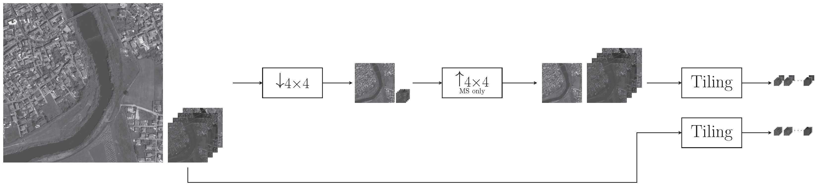
Given the excellent performance of the super-resolution method proposed in [36] we decided to apply the same approach to the pansharpening problem. However, we also want to take advantage of the large domain-specific knowledge existing on remote sensing image processing, introducing some reasonable changes aimed at better exploiting the data. Accordingly, in the following, we first provide some details about the targeted datasets, then we describe the basic architecture, directly inherited from the super-resolution method, and finally, based on a first analysis of results, we propose our remote-sensing specific solution.

3.1. Datasets

The proposed method, although rather general, it has been conceived for very high resolution data, and in particular it has been tested on data acquired by some of the most advanced systems for remote sensing of optical data. These are Ikonos, GeoEye-1, and WorldView-2, whose main characteristics are summarized in

Table 1. Spatial resolutions for Ikonos, GeoEye-1, and WorldView-2 sensors.

	PAN	MS
Ikonos	0.82 m GSD at nadir	3.28 m GSD at nadir
GeoEye-1	0.46 m GSD at nadir	1.84 m GSD at nadir
WorldView-2	0.46 m GSD at nadir	1.84 m GSD at nadir

and

Table 2. Spectral bands of Ikonos, GeoEye-1, and WorldView-2 sensors. When the band is comprised the wavelength range (in nm) is reported.

	PAN	Coastal	Blue	Green	Yellow	Red	Red Edge	Nir	Nir 2
Ikonos	526–929	no	445–516	506–595	no	632–698	no	757–853	no
GeoEye-1	450–900	no	450–520	520–600	no	625–695	no	760–900	no
WorldView-2	450–800	400–450	450–510	510–580	585–625	630–690	705–745	770–895	860–1040

. This sensors selection allowed us to study the robustness of the proposed method with respect to both spectral resolution (Ikonos/GeoEye-1 vs. WorldView-2) and spatial resolution (Ikonos vs. GeoEye-1/WorldView-2).

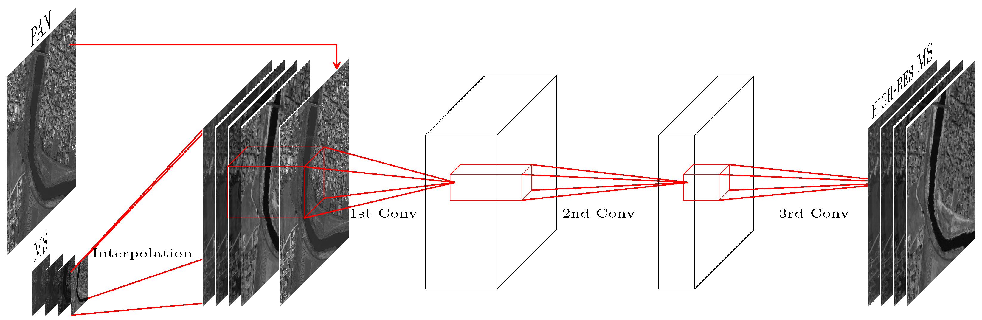
3.2. Basic Architecture

Figure 1 provides a pictorial representation of the basic architecture, which follows closely the super-resolution CNN (SRCNN) architecture. The example is tailored on Ikonos and GeoEye-1 data, with 4-band multispectral components and a panchromatic band with $4\times 4$ higher spatial resolution, but applies to other multi-resolution data with obvious modifications. The four low-resolution spectral bands are first upsampled ($4\times 4$) and interpolated. The result is then stacked with the high-resolution panchromatic band to form the 5-component input. Hence, the network will work at the target resolution from the beginning, with no need of up/down-sampling. The output comprises only 4 bands, which correspond to the input multispectral bands, but at the target panchromatic resolution. We keep using the three-layer structure of [36], but replace the $1\times 1$ kernels of the central layer with $5\times 5$ kernels as, again, these provide some performance improvements in preliminary experiments.

Table 3. Default CNN architecture in case of a multispectral component with $B=4$ bands and without external features. $c_1$ is the total number of input bands.

$c_1=B+1$	$K_1\times K_1$	$f_1\left(x\right)$	$c_2$	$K_2\times K_2$	$f_2\left(x\right)$	$c_3$	$K_3\times K_3$	$f_3\left(x\right)$	$c_4=B$
5	$9\times 9$	ReLU	64	$5\times 5$	ReLU	32	$5\times 5$	x	4

summarizes the parameters of the overall architecture. It is worth underlining that this is quite a simple CNN architecture, relatively shallow, and hence easy to train with a limited training set. This is extremely important for the remote sensing field, where training data are often scarce as opposed to the millions images typically available for computer vision applications. We will therefore stick to this three-layer architecture also in the following, adapting it to remote sensing pansharpening based on prior knowledge on the problem, and working only on the input data.

Turning to implementation details, the output of the CNN is a B-band multispectral image with the same spatial resolution as the PAN component. This image should be as close as possible to the ideal image acquired by a multispectral sensor operating at the same spatial resolution of the PAN. Of course, this latter image does not exist. This raises problems not only for performance assessment but, in deep learning, also for network training. We will address both problems using the Wald protocol [41], which consists in working on a downsampled multi-resolution image, for which the original MS component represents a valid reference.

Training based on the Wald training protocol is summarized in Figure 2. In the upper channel, the original image is downsampled, then its MS component is interpolated, and the resulting $(B+1)$ image is tiled and fed to the CNN. In the lower channel, the original MS component is itself tiled and used as a reference. During training, the CNN parameters are adapted to produce output tiles that match as closely as possible the reference tiles. The learned parameters are eventually used for the pansharpening of the real multiresolution images, at their original resolution. Clearly, the whole procedure rests upon the hypothesis that performance does not depend critically on scale, which is not always the case, as discussed in the Introduction. Therefore, to reduce the possible mismatches, we smooth data before downsampling, following [2,22], using a filter that matches the modulation transfer function of the sensor. Likewise, we upsample the MS component using the interpolation kernel proposed in [13]. In any case, great attention must be devoted to assess performance not only on the low-resolution data but also on the original images.

Learning has been carried out as proposed in [36] and we used exactly the same setting, briefly summarized here. It is based on backpropagation with stochastic gradient descent. The updating iteration refers to a batch of 128 input tiles selected at random from the training set. As loss function L, we use the mean square error between the pansharpened tile $\widehat{X}$ and its reference X, averaged on the batch (To account for the border effects of the filtering, suitably cropped versions of $\widehat{X}$ and X are involved in the computation).

$$L\left(W\right)=\frac{1}{128}\sum _{n=1}^{128}\left|\right|X_n-{\widehat{X}}_n\left(W\right){\left|\right|}^2$$

(4)

where W is the set of all parameters, namely, filter weights and biases. Stochastic gradient descent uses a momentum parameter to reduce randomness, therefore, iteration $(i+1)$ reads as

$$W_{i+1}=W_i+\Delta W_i=W_i+\mu ·\Delta W_{i-1}-\alpha ·\nabla L_i$$

(5)

where μ is the momentum, and α the learning rate. Following the indications given in [36] we set $\mu =0.9$ and $\alpha ={10}^{-4}$, except for the last layer, where we set $\alpha ={10}^{-5}$, since a smaller learning rate is known to speed up convergence. In all cases the total number of iterations has been fixed to 1.12 × ${10}^6$. Additional details about learning can be found in [36].

Figure 3 shows a sample result of the proposed pansharpening method. On the left, there is the input multiresolution image, acquired by the GeoEye-1 sensor, with PAN and MS components at their actual scales (all MS images, here and in the following, are projected on a suitable RGB space). On the right, the result of the pansharpening process, and in the center, for reference the interpolated multispectral component. The result looks quite satisfactory: the spatial resolution of the PAN component is fully preserved, and colors, when the comparison makes sense, are very similar to those of the interpolated MS component, suggesting the absence of spectral distortions. In Section 4, this positive judgement will be supported by strong numerical evidence.

3.3. Remote-Sensing Specific Architecture

Although the basic architecture provides already very good results, we set to analyze in more depth its behavior over remote sensing imagery with the goal to propose some sensible improvements based on the available prior knowledge. In particular, we focus on the first-layer filters, whose behavior may be interpreted quite easily, while this is much more difficult for layers further away from the input.

With reference to WorldView-2 images, hence with nine input bands, Figure 4a plots the energy of the feature maps at the output of the first layer, sorted in decreasing order. A sharp energy drop is visible after feature 48, suggesting that some of the filters are not really capturing valuable information, and could be removed altogether. This interpretation is reinforced by the analysis of the filter responses, some of which are shown in Figure 5. In each column, we show the $9\times 9$ spatial kernels associated with the 8 spectral components of the input plus the panchromatic component, recalled with an abbreviation on the left. For the sake of clarity, we only show some high-energy filters, on the left, and then some filters around the transition highlighted before. Filters beyond #48 exhibit noise-like kernels, confirming that they are not matching relevant features, and are not effectively trained by the network [42]. On the contrary, the other filters exhibit well-defined patterns. Spatial structures emerge mainly in the last component, associated with the panchromatic band, while kernels associated with spectral bands are spatially smooth. This is clearly due to the different resolutions of the original bands. Instead, the components associated with spectral bands show strong energy variations, suggesting spectral selectivity. In practice, they are extracting spectral signatures associated with the image land covers. For example, filter #7 matches quite well the vegetation. In fact, a well known indicator for vegetation is the normalized difference vegetation index (NDVI), see Equation (7), which basically computes a normalized difference between responses in near-infrared and red bands. Accordingly, filter #7 has a strongly positive kernel in the 7th patch, associated with the near-infrared component, and negative in the 5th patch, associated with the red component. Similar considerations apply to filter #48 which correlates to the water signature. In fact it differentiates between the first three spectral bands (coastal, red, and green) and those from 6th to 8th (near infrared). Notably, this matches pretty well the definition of the normalized difference water index (NDWI), see Equation (6). (This filter has very small energy because of the scarcity of water samples in the dataset used for training. This is confirmed by the noisy shape of the filter that indicates the need of further training to increase its regularity. However, the network is quite robust anyway, as other filters match the water class, although less obviously than filter #48.)

Figure 6 provides further insight into this interpretation. It shows, on the left, a color image obtained by combining three suitable bands of a WorldView-2 image, and then the feature maps associated with filter #7 (center) and filter #48 (right). In the first map, all vegetated areas are clearly highlighted, although some “errors” of interpretation can also be spotted in the top-left part of the image. Likewise, the second map highlights very clearly water basins, again, with some scattered “errors”.

Beyond the two above mentioned feature maps, many more, both in the first and the second layer, exhibit a remarkable correlation with some class-specific radiometric indexes. This interesting behavior, with the network trying to mimic well-established features, has motivated us to add some such indexes in order to “guide” (and hopefully boost) the learning process. Indeed, this intuition was supported by experimental results. A possible explanation lies in the relative invariance of the normalized indexes with respect to the illumination. Invariance, in fact, improves the network capability to “generalize” and hence to perform well on data which are scarcely (or not at all) represented in the training set. Therefore, based on numerical results and on the above considerations, we augmented the input by adding further planes, corresponding to some well-known indices. In particular, we considered the following nonlinear radiometric indices computed from the multispectral components (see also Table 2):

• Normalized Difference Water Index:

  $${\mathrm{NDWI}}_{\mathrm{Ikonos}/\mathrm{GeoEye}-1}=\frac{Green-Nir}{Green+Nir}; {\mathrm{NDWI}}_{\mathrm{WorldView}-2}=\frac{Coastal-Nir2}{Coastal+Nir2}$$

  (6)
• Normalized Difference Vegetation Index:

  $${\mathrm{NDVI}}_{\mathrm{Ikonos}/\mathrm{GeoEye}-1}=\frac{Nir-Red}{Nir+Red}; {\mathrm{NDVI}}_{\mathrm{WorldView}-2}=\frac{Nir2-Red}{Nir2+Red}$$

  (7)
• Normalized Difference Soil Index (applies to WorldView-2 only):

  $${\mathrm{NDSI}}_{\mathrm{WorldView}-2}=\frac{Green-Yellow}{Green+Yellow}$$

  (8)
• Non-Homogeneous Feature Difference (applies to WorldView-2 only):

  $${\mathrm{NHFD}}_{\mathrm{WorldView}-2}=\frac{Red Edge-Coastal}{Red Edge+Coastal}$$

  (9)

Radiometric indices can be defined in many different ways [43], and indeed we use different definitions of NDVI and NDWI for the four-band (Ikonos/GeoEye-1) and 8-band (WorldView-2) images, since number and meaning of the bands change. Moreover, two of the indexes are defined only for the richer WorldView-2 images. More indices proposed in the remote sensing community could be tested, but selecting the most informative of them goes outside the scope of this work.

Figure 4b shows the distribution of filter energy after augmenting the input with the nonlinear radiometric indices. The number of inactive filters drops from 16 to 9, and several filters correlate well with the new indices. Moreover, filter energy grows in general, also for filters that were already active. These facts seem to support our conjecture that the remote sensing specific features do serve as a guidance for the network, allowing it to better address the pansharpening task. A stronger support will come from experimental evidence.

Besides augmenting the input, we tested further minor variations to the basic architecture, modifying the number of filters and their spatial support. Although a wide range of alternative architectures have been tested, we will focus on a meaningful subset of them obtained by changing the hyperparameters $B_{\mathrm{rad}}$ (hence $c_1$), $K_1$, and $c_2$ as summarized in

Table 4. Hyper-parameters of the CNN architectures for Pansharpening. $B_{\mathrm{rad}}$: number of nonlinear radiometric indices, $K_1\times K_1$: spatial support of first-layer filters, $c_2$ number of first-layer filters.

Sensor	B	$B_{\mathrm{rad}}$	$c_1=B+B_{\mathrm{rad}}+1$	$K_1$	$c_2$
Ikonos, GeoEye-1	4	$\{0,2\}$	$\{5,7\}$	$\{5,9,15\}$	$\{48,56,64\}$
WorldView-2	8	$\{0,4\}$	$\{9,13\}$	$\{5,9,15\}$	$\{48,56,64\}$

. Changes in the second and the third layers have also been tested but eventually discarded, as ineffective.

4. Results and Discussion

Several experiments have been carried out to find the optimal setting for the proposed technique and assess its performance in comparison with several state-of-the-art references. To this end, three datasets have been designed, with images acquired by the Ikonos, GeoEye-1 and WorldView-2 multiresolution sensors, all characterized by a very high spatial resolution, below one meter for the panchromatic band (sensor characteristics are summarized in Table 1 and Table 2). In all cases, the MS component has spatial resolution $4\times 4$ lower than the PAN. Datasets are divided (see

Table 5. Datasets partition.

	Training	Validation	Test
Ikonos	$14400\times (33\times 33)$	$7168\times (33\times 33)$	$50\times (320\times 320)$
GeoEye-1	$14400\times (33\times 33)$	$7168\times (33\times 33)$	$70\times (320\times 320)$
WorldWiew-2	$14400\times (33\times 33)$	$7168\times (33\times 33)$	$30\times (320\times 320)$

) in disjoint training, validation and test subsets. The first two subsets are used for CNN training, while the last one is used for performance assessment of all techniques.

For performance assessment, we use a number of metrics proposed in the literature, since no single one can be considered by itself as a reliable indicator of quality. In particular, besides several full-reference metrics, which measure performance on the reduced resolution dataset according to the Wald protocol, we consider also the no-reference QNR [44] and two derived metrics, that work on the full-resolution dataset. In fact, while these latter indicators may be considered less objective than the former, they are insensitive to possible scale-related phenomena. In

Table 6. Full-reference (low resolution) and no-reference (full resolution) performance metrics.

full reference	SAM	Spectral Angle Mapper [45]
	ERGAS	Erreur Relative Globale Adimensionnelle de Synthèse [46]
	SCC	Spatial Correlation Coefficient [47]
	Q	Universal Image Quality index [48] averaged over the bands
	Qx	x-band extension of Q [49]
no reference	QNR	Quality with no-Reference index [44]
	${\mathbf{D}}_{\mathbf{\lambda }}$	Spectral component of QNR
	${\mathbf{D}}_{\mathit{S}}$	Spatial component of QNR

, all these metrics are listed together with the corresponding reference for the interested reader.

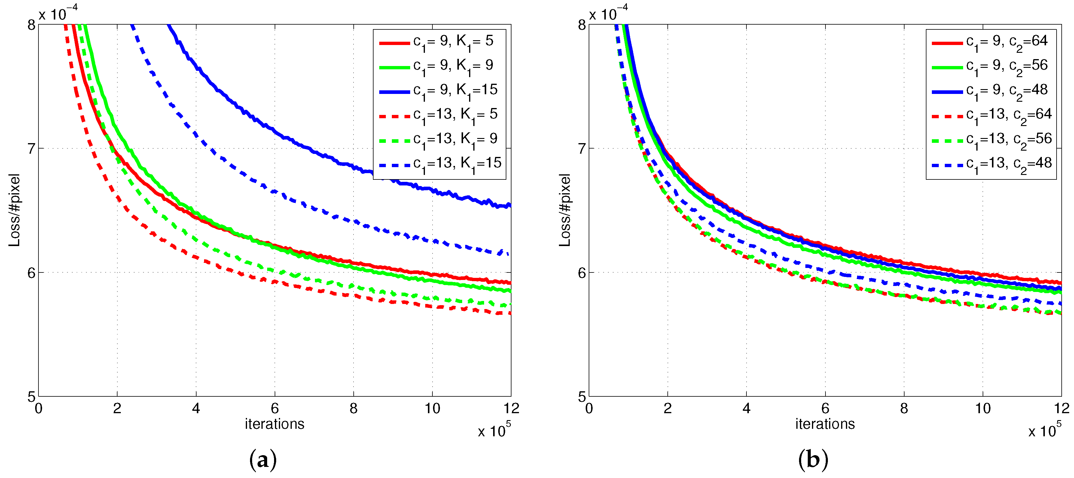
4.1. Comparing Different Networks

In this subsection we report the results of a series of experiments aimed at finding optimal settings for the proposed method, both with and without the external features derived from nonlinear radiometric indices.

Table 7. Performance of various configurations of the proposed architecture on WorldView-2 images without (top) and with (bottom) nonlinear radiometric indices. Best result in red and blue, respectively.

			Q4	Q	SAM	ERGAS	SCC	${\mathrm{D}}_{\lambda }$	${\mathrm{D}}_S$	QNR
$c_1$	$K_1$	$c_2$	$\to 1$	$\to 1$	$\to 0$	$\to 0$	$\to 1$	$\to 0$	$\to 0$	$\to 1$
9	5	48	0.8518	0.9445	2.5750	1.6031	0.9405	0.0190	0.0551	0.9269
		56	0.8519	0.9446	2.5754	1.6028	0.9403	0.0198	0.0557	0.9256
		64	0.8514	0.9440	2.5867	1.6055	0.9402	0.0192	0.0552	0.9267
	9	48	0.8500	0.9438	2.6034	1.6147	0.9402	0.0209	0.0522	0.9280
		56	0.8515	0.9441	2.5851	1.6045	0.9403	0.0206	0.0522	0.9283
		64	0.8520	0.9445	2.5703	1.6016	0.9403	0.0199	0.0532	0.9280
	15	64	0.8448	0.9413	2.6671	1.6615	0.9370	0.0232	0.0534	0.9248
13	5	48	0.8528	0.9449	2.5483	1.5844	0.9413	0.0200	0.0523	0.9287
		56	0.8537	0.9449	2.5454	1.5783	0.9418	0.0181	0.0525	0.9303
		64	0.8539	0.9452	2.5390	1.5792	0.9419	0.0181	0.0521	0.9308
	9	48	0.8511	0.9442	2.5767	1.6029	0.9392	0.0199	0.0485	0.9326
		56	0.8527	0.9450	2.5570	1.5898	0.9412	0.0194	0.0497	0.9319
		64	0.8525	0.9448	2.5585	1.5899	0.9414	0.0186	0.0508	0.9316
	15	64	0.8472	0.9425	2.6263	1.6413	0.9392	0.0213	0.0508	0.9290

reports the performance achieved on WorldView-2 images as a function of the parameters $c_1,K_1$, and $c_2$. In this case, $c_1$, the number of input bands, may be only 9 (without external features) or 13 (with them). For the first-layer filters, with support $K_1\times K_1$, we tested small, medium and relatively large receptive fields, with $K_1=5, 9$ and 15, respectively. Finally, we have considered $c_2=48, 56$ or 64 features at the output of the first layer.

In both cases, with and without external features, using large filters, $K_1=15$, causes some performance loss. This can be easily explained by looking at Figure 7a, showing the evolution of the loss function (computed on the validation set) during training. Apparently ${10}^6$ iterations are not enough to reach convergence with $K_1$ = 15. On the other hand, even at convergence (after four millions iterations), results are just on par with the other cases. This is likely due to overfitting problems, typically occurring when the training dataset is not large enough, as well explained in [42]. This same limitation observed in width applies in depth as well, as already pointed out in [36] for the super-resolution problem. It would be certainly interesting to test more complex networks, e.g., with larger supports and/or deeper architectures, as we may observe more complex filter’s patterns than those shown in Figure 5, but lacking a proportionally larger dataset (not available in this work) for training it would not make sense. Therefore, in particular, we decided not to investigate the $K_1=15$ option further. Concerning the comparison between $K_1=5$ and $K_1=9$, results indicate clearly that the former choice improves spectral accuracy (see ${\mathbf{D}}_{\lambda }$), and the latter spatial accuracy (see ${\mathbf{D}}_S$), as could be expected. As for the number of output features, they can be reduced from 64 to 48 with no significant accuracy loss, especially in case no external features are used. Finally, let us focus on the comparison between $c_1=9$, and $c_1=13$, that is, on the impact of external radiometric indices. To this end, we have highlighted in color the best result for each indicator both for $c_1=9$ (red, in the upper part of the table) and for $c_1=13$ (blue, in the lower part). The injection of external features improves consistently the best performance. This behavior is also confirmed by the analysis of Figure 7, showing loss function evolution for architectures with different filter support (left) and number of output features (right) with and without radiometric indices. For each basic configuration (solid line), the corresponding architecture with augmented input (dashed line) provides a significant reduction of the loss.

In

Table 8. Performance of various configurations of the proposed architecture on Ikonos images without (top) and with (bottom) nonlinear radiometric indices. Best result in red and blue, respectively.

			Q4	Q	SAM	ERGAS	SCC	${\mathrm{D}}_{\lambda }$	${\mathrm{D}}_S$	QNR
$c_1$	$K_1$	$c_2$	$\to 1$	$\to 1$	$\to 0$	$\to 0$	$\to 1$	$\to 0$	$\to 0$	$\to 1$
5	5	48	0.7557	0.8970	2.3199	1.6693	0.9384	0.0569	0.0768	0.8713
		56	0.7565	0.8974	2.3170	1.6681	0.9386	0.0547	0.0791	0.8712
		64	0.7562	0.8970	2.3223	1.6629	0.9386	0.0538	0.0798	0.8713
	9	48	0.7565	0.8970	2.3149	1.6569	0.9401	0.0602	0.0725	0.8719
		56	0.7575	0.8979	2.3071	1.6521	0.9404	0.0613	0.0768	0.8672
		64	0.7581	0.8981	2.3068	1.6537	0.9404	0.0617	0.0764	0.8672
7	5	48	0.7609	0.9006	2.2831	1.6634	0.9411	0.0514	0.0731	0.8796
		56	0.7607	0.9003	2.2774	1.6547	0.9413	0.0527	0.0733	0.8782
		64	0.7611	0.9005	2.2737	1.6544	0.9409	0.0525	0.0731	0.8786
	9	48	0.7613	0.8997	2.2743	1.6380	0.9422	0.0568	0.0720	0.8757
		56	0.7616	0.9003	2.2645	1.6339	0.9427	0.0589	0.0737	0.8722
		64	0.7616	0.9004	2.2658	1.6335	0.9425	0.0573	0.0733	0.8740

and

Table 9. Performance of various configurations of the proposed architecture on GeoEye-1 images without (top) and with (bottom) nonlinear radiometric indices. Best result in red and blue, respectively.

			Q4	Q	SAM	ERGAS	SCC	${\mathrm{D}}_{\lambda }$	${\mathrm{D}}_S$	QNR
$c_1$	$K_1$	$c_2$	$\to 1$	$\to 1$	$\to 0$	$\to 0$	$\to 1$	$\to 0$	$\to 0$	$\to 1$
5	5	48	0.8090	0.9395	2.1582	1.5953	0.9117	0.0354	0.0700	0.8974
		56	0.8065	0.9388	2.1658	1.6052	0.9106	0.0377	0.0682	0.8970
		64	0.8089	0.9398	2.1562	1.5994	0.9116	0.0365	0.0683	0.8979
	9	48	0.8089	0.9394	2.1597	1.5836	0.9134	0.0394	0.0672	0.8964
		56	0.8097	0.9403	2.1416	1.5688	0.9147	0.0377	0.0663	0.8988
		64	0.8094	0.9398	2.1494	1.5742	0.9145	0.0346	0.0652	0.9028
7	5	48	0.8112	0.9401	2.1249	1.5689	0.9167	0.0340	0.0650	0.9034
		56	0.8089	0.9398	2.1360	1.5889	0.9146	0.0337	0.0648	0.9040
		64	0.8088	0.9401	2.1296	1.5843	0.9154	0.0344	0.0663	0.9018
	9	48	0.8094	0.9402	2.1311	1.5661	0.9152	0.0327	0.0611	0.9084
		56	0.8112	0.9403	2.1299	1.5598	0.9153	0.0333	0.0626	0.9065
		64	0.8103	0.9400	2.1364	1.5605	0.9151	0.0345	0.0603	0.9075

we report results obtained on the other two datasets. Apart from numerical differences, it seems safe to say that the same phenomena observed for the WorldView-2 dataset emerge also in these cases.

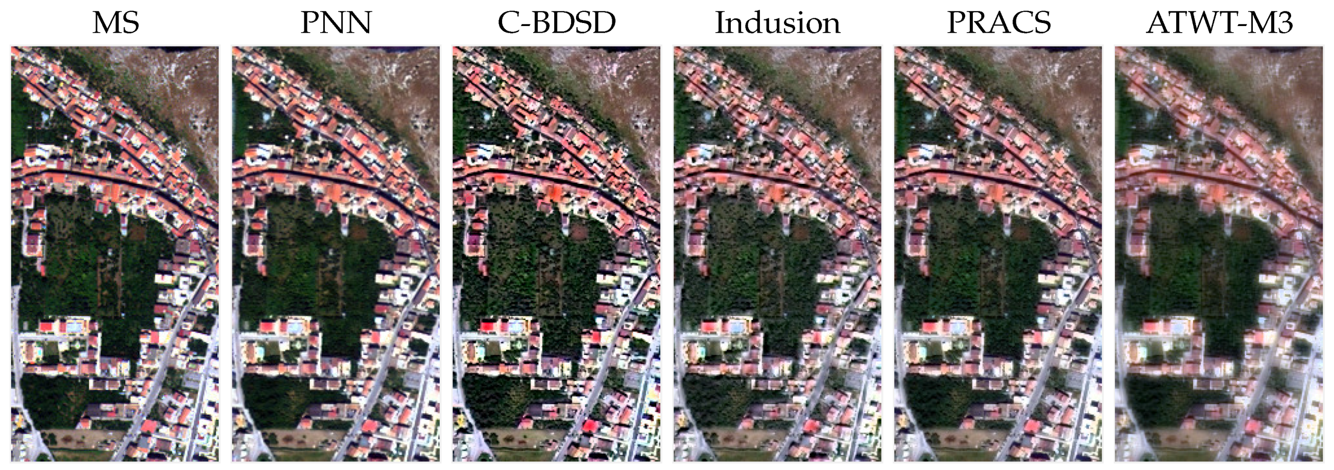
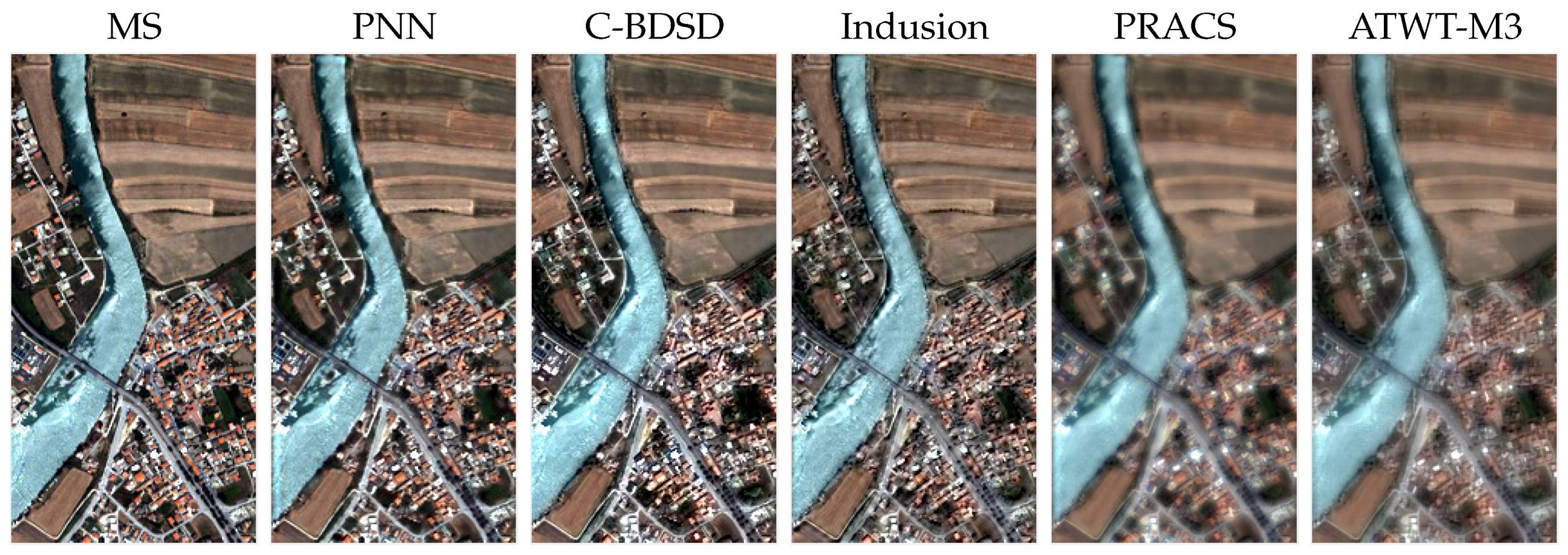
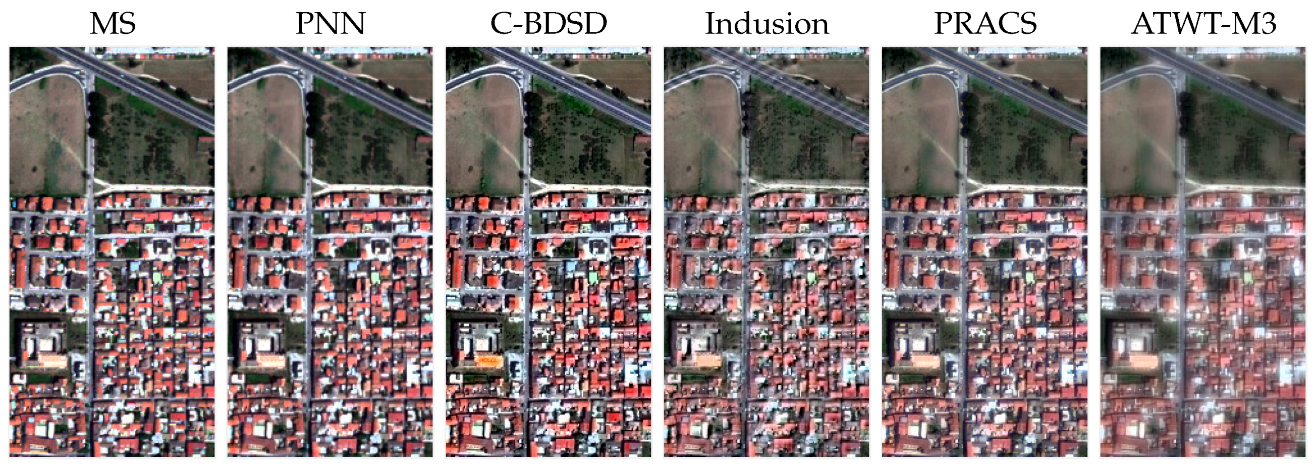
4.2. Comparison with the State of the Art

Let us now compare the proposed method (using the acronym PNN in the following, for CNN-based Pansharpening) with a number of state-of-the-art reference techniques. We tested all the techniques analyzed in the recent review paper [2], whose implementation has been made available online [50]. However, in the following tables, we report results only for the most competitive ones, listed below, according to the quality indices adopted.

• PRACS: Partial Replacement Adaptive Component Substitution [10];
• Indusion: Decimated Wavelet Transform using an additive injection model [18];
• AWLP: Additive Wavelet Luminance Proportional [20], a generalization of AWL [19];
• ATWT-M3: A Trous Wavelet Transform with the injection Model 3 proposed in [15];
• MTF-GLP-HPM: Generalized Laplacian Pyramid with MTF-matched filter and multiplicative injection model [16];
• BDSD: Band-Dependent Spatial-Detail with local parameter estimation [25];
• C-BDSD: A non-local extension of BDSD, proposed in [26].

We included the recently proposed C-BDSD technique [26], since this is an improvement of BDSD, already among the best references. This has been implemented and configured according to the author’s indications. As for the proposed method, we selected for each dataset the architecture which provided the best QNR figure, always with the nonlinear radiometric indices included. With this choice we decided to give more emphasis to full-resolution results, more indicative of real-world operation, although obtained with a no-reference metric. Software and implementation details will be made available online [51] to ensure full reproducibility. Again, we provide results separately for the three datasets in

Table 10. Performance comparison on the WorldView-2 dataset.

	Q4	Q	SAM	ERGAS	SCC	${\mathrm{D}}_{\lambda }$	${\mathrm{D}}_S$	QNR
	$\to 1$	$\to 1$	$\to 0$	$\to 0$	$\to 1$	$\to 0$	$\to 0$	$\to 1$
PRACS	0.7908	0.8789	3.6995	2.4102	0.8522	0.0234	0.0734	0.9050
Indusion	0.6928	0.8373	3.7261	3.2022	0.8401	0.0552	0.0649	0.8839
AWLP	0.8127	0.9043	3.4182	2.2560	0.8974	0.0665	0.0849	0.8549
ATWT-M3	0.7039	0.8186	4.0655	3.1609	0.8398	0.0675	0.0748	0.8628
MTF-GLP-HPM	0.8242	0.9083	3.4497	2.0918	0.9019	0.0755	0.0953	0.8373
BDSD	0.8110	0.9052	3.7449	2.2644	0.8919	0.0483	0.0382	0.9156
C-BDSD	0.8004	0.8948	3.9891	2.6363	0.8940	0.0251	0.0458	0.9304
PNN	0.8511	0.9442	2.5767	1.6029	0.9392	0.0199	0.0485	0.9326

,

Table 11. Performance comparison on the Ikonos dataset.

	Q4	Q	SAM	ERGAS	SCC	${\mathrm{D}}_{\lambda }$	${\mathrm{D}}_S$	QNR
	$\to 1$	$\to 1$	$\to 0$	$\to 0$	$\to 1$	$\to 0$	$\to 0$	$\to 1$
PRACS	0.6597	0.8021	2.9938	2.3597	0.8735	0.0493	0.1148	0.8424
Indusion	0.5928	0.7660	3.2800	2.7961	0.8506	0.1264	0.1619	0.7340
AWLP	0.7143	0.8389	2.8426	2.1126	0.9069	0.1384	0.1955	0.6951
ATWT-M3	0.5579	0.7249	3.5807	3.0327	0.8183	0.1244	0.1452	0.7490
MTF-GLP-HPM	0.7178	0.8422	2.8820	2.0550	0.9072	0.1524	0.2186	0.6646
BDSD	0.7199	0.8576	2.9147	1.9852	0.9084	0.0395	0.0884	0.8761
C-BDSD	0.7204	0.8569	2.9101	2.0553	0.9164	0.0710	0.1218	0.8173
PNN	0.7609	0.9006	2.2831	1.6634	0.9411	0.0514	0.0731	0.8796

and

Table 12. Performance comparison on the GeoEye-1 dataset.

	Q4	Q	SAM	ERGAS	SCC	${\mathrm{D}}_{\lambda }$	${\mathrm{D}}_S$	QNR
	$\to 1$	$\to 1$	$\to 0$	$\to 0$	$\to 1$	$\to 0$	$\to 0$	$\to 1$
PRACS	0.6995	0.8568	3.2364	2.4296	0.8113	0.0470	0.0877	0.8698
Indusion	0.5743	0.7771	3.5361	3.5480	0.7600	0.1270	0.1262	0.7651
AWLP	0.7175	0.8615	3.6297	2.6134	0.7878	0.1247	0.1521	0.7436
ATWT-M3	0.6008	0.7907	3.5546	3.0729	0.7944	0.0712	0.0710	0.8633
MTF-GLP-HPM	0.7359	0.8718	3.2205	5.0344	0.7887	0.1526	0.1815	0.6956
BDSD	0.7399	0.8832	3.3384	2.2342	0.8526	0.0490	0.0994	0.8572
C-BDSD	0.7391	0.8784	3.4817	2.4370	0.8591	0.0832	0.1342	0.7953
PNN	0.8094	0.9402	2.1311	1.5661	0.9152	0.0327	0.0611	0.9084

. Performance figures are obtained by averaging over all test images of the dataset.

Numerical results speak very clearly in favor of the proposed solution. Let us focus, for the time being, on the WorldView-2 dataset, as in Table 10. Under all full-reference metrics, CNN-based pansharpening guarantees a large performance gain with respect to all references, with MTF-GLP-HPM taking the role of the closest challenger. The situation changes somewhat with no-reference full-resolution measures, where the gap is more narrow and in a single case, for metric ${\mathbf{D}}_S$, BDSD exhibits a better performance. Notice also that, with these metrics, MTF-GLP-HPM becomes the worst reference, while BDSD and C-BDSD are very competitive. This sheds further light on the importance of using multiple metrics and of using careful visual inspection to complement numerical indications. Notice also that, with the exception of BDSD and C-BDSD for no-reference metrics, the performance gap between the proposed solution and all references is much wider than the gap among the various tested CNN architectures, testifying on the robustness of this approach versus the selected hyperparameters.

The analysis of results obtained on the other datasets, reported in Table 11 and Table 12, highlights some differences in the behavior of reference techniques, but the proposed solution keeps being largely preferable, especially for GeoEye-1 data, where the gap with all competitors, including BDSD and C-BDSD, becomes very large, even for no-reference metrics.

To add a further piece of information,

Table 13. Average ranking over test images for a few metrics.

	WorldView-2			Ikonos			GeoEye-1
	Q4	SAM	QNR	Q4	SAM	QNR	Q4	SAM	QNR
PRACS	5.0	4.3	3.7	5.8	4.2	3.0	5.6	3.5	3.1
Indusion	7.6	4.2	4.5	7.0	4.9	5.6	7.6	4.9	5.9
AWLP3.7	3.8	2.6	6.5	3.7	2.2	6.7	4.8	3.0	6.7
ATWT-M3	7.4	6.0	6.4	7.8	7.0	5.3	7.3	5.9	2.9
MTF-GLP-HPM	2.5	2.8	7.7	3.2	2.8	8.0	3.1	3.1	8.0
BDSD	3.7	8.0	3.3	3.7	6.5	2.1	3.1	7.8	3.0
C-BDSD	5.0	7.0	2.0	3.4	7.2	3.4	3.5	6.8	5.0
PNN	1.0	1.2	1.9	1.2	1.0	1.9	1.0	1.0	1.4

reports, for each dataset, and for some of the performance metrics considered before, the ranking of the compared techniques averaged over all test images. Considering full-reference metrics, the proposed method proves almost always best over the images of all datasets. Only with the no-reference metric QNR, and for two datasets out of three, BDSD or C-BDSC happen to be preferable for some images, although the proposed solution keeps being the first choice on average. It also worth noting that the proposed solution is robust with respect to data resolution. Considering the original datasets, and their 4 × 4 subsampling, our experiments spanned a resolution range of three octaves, with the proposed method outperforming consistently all references. A further performance gain could be achieved by relaxing the constraint on the number of iterations (at the cost of increased design time), as obvious by Figure 7 where the loss functions is not yet at convergence. Finally, as for all machine learning methods, the availability of more training data would certainly benefit performance and robustness.

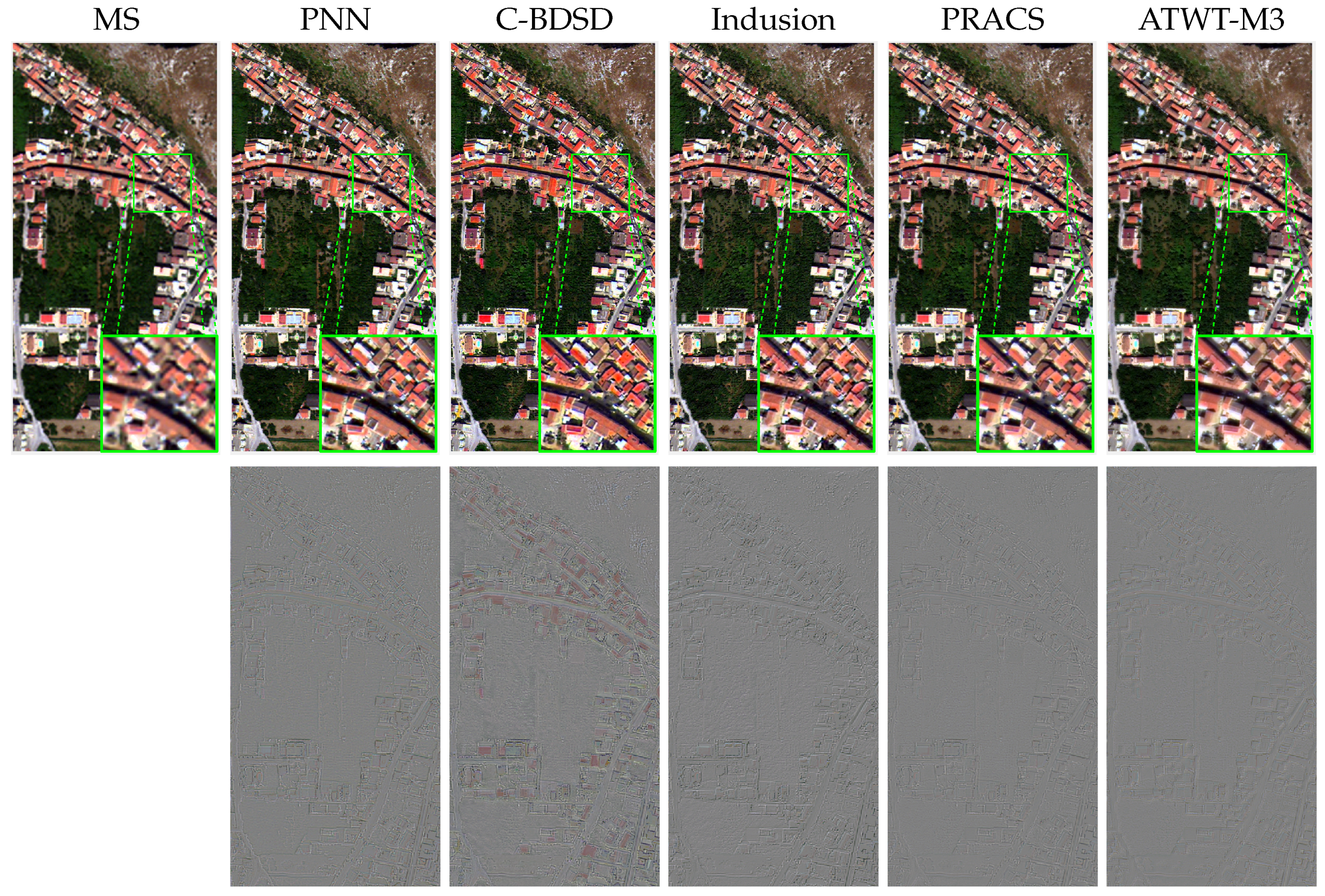
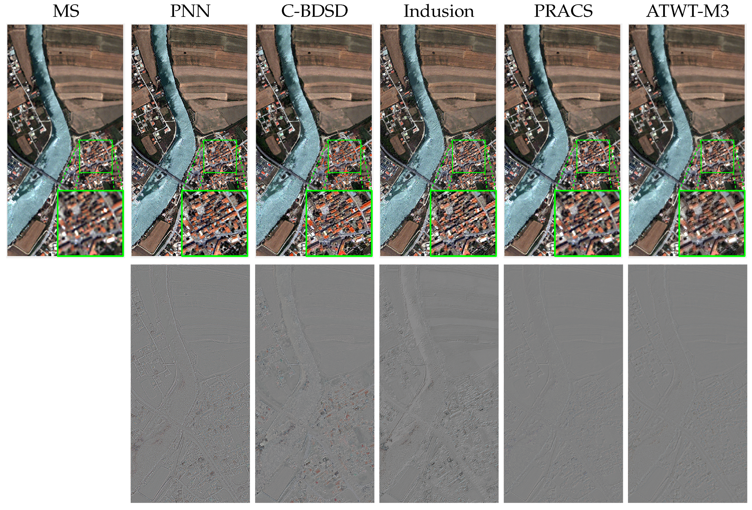
4.3. Visual Inspection

We conclude our analysis with a careful visual inspection of results. Numerical indicators, in fact, represent only proxies for quality, especially useful during development phases. Only visual inspection allows one to discover a number of artifacts and distortions that elude quantitative analyses. Therefore, for each dataset, we selected a sample image including both urban and natural areas, to allow for a meaningful comparison of pansharpening quality among competing techniques. Together with the reference image, we show (Images should be analyzed on a computer screen with suitable zoom) the output of the proposed method and of a subset of references, chosen for their variety and good objective performance.

First, in Figure 8, Figure 9 and Figure 10, we show the low-resolution versions, used to compute full-reference metrics by the Wald protocol. For these images, a valid reference exists, namely, the original multispectral component, shown on the left. The pansharpened images produced by the proposed method look very similar to the original MS components, with comparable spatial resolution and without noticeable artifacts or spectral distortions. C-BDSD returns images which look even sharper than the original, with many more high-frequency details, for example in the vegetation areas. Therefore it seems to provide an enhanced version of the target image. It may be debated, though, whether this is desirable for a pansharpening method. For sure, all images, and markedly the GeoEye-1, present a significant spectral distortion, especially visible in the rooftops. Indusion is characterized by a subtle diffused blurring and some strong artifacts, see the highway in the GeoEye-1 image. The behavior of PRACS is not uniform over the images, it works quite well on the WolrdView-2 and GeoEye-1 images, but introduces a very strong blurring in the Ikonos image. ATWT-M3, on the contrary, provides images of consistently very low quality, with intense blurring, arguably worse than the low-resolution original. This, despite the relatively good performance in terms of no-reference metrics. On the other hand, as will be soon obvious, the performance of ATWT-M3 on the actual data is not nearly as bad, raising further alarm on metric reliability, especially in the presence of scale issues.

In Figure 11, Figure 12 and Figure 13, we show the actual full-resolution images obtained through pansharpening. This time, no ground truth exists. However, we show on the left as reference the up-sampled MS component with bicubic interpolation. By comparison, one can appreciate the new details introduced by pansharpening and, at the same time, spot possible spectral distortion in homogeneous regions. As a general remark, most pansharpened images exhibit a very good quality, with an impressive improvement with respect to interpolated MS, especially visible in the enlarged box. In particular, the proposed method appears as one of the more effective, with a consistent performance over all sensors. At a closer inspection, however, a number of problems emerge again. For the proposed method, a subtle pattern is visible is some homogeneous areas, probably related to the high-degree interpolation polynomial. C-BDSD, as before, is mainly affected by spectral distortion, with a clear over-saturation, specially for the green and red hues. Indusion exhibits significant spatial distortion (mostly, ringing artifacts) in the urban areas, while PRACS (in the Ikonos image) and ATWT-M3 (always) introduce spatial blurring, although less than in the low-resolution case. All these observations are also supported by the detail images (difference between pansharpened image and interpolated reference) shown in the bottom row of each figure. The colored areas in the C-BDSD detail images testify of the mentioned spectral distortion, while the low energy of the the PRACS and especially ATWT-M3 detail images underline the inability of these techniques to inject all necessary high-resolution details in the pansharpened image.

4.4. Implementation Details

To conclude this section we provide some implementation details for the proposed method. All implemented PNNs have approximatively the same complexity, and actually they take about the same amount of computational burden in both learning and testing phases. In particular, the learning phase takes about half a day and is carried on GPU (Nvidia Tesla K20c with CUDA 7.5 and CuDNN v3) through the deep learning framework Caffe [52]. The testing of any PNN, instead, performed via CPU (PC with 2GHz Intel Xeon processor and 64 Gb) and implemented in MATLAB by means of MatConvNet [53], on a $320\times 320$ (in the MS domain) image takes about 20 seconds, which is comparable to the time required by reference algorithms.

5. Conclusions

Deep learning has proven extremely effective in a large number of image processing and computer vision problems. Based on this observation, we decided to use convolutional neural networks to address the pansharpening task, modifying an architecture recently proposed for super-resolution. To improve performance without resorting to data-intensive deeper architectures, which would call for huge training sets and complexity, we augmented the input by including several maps of nonlinear radiometric indices. This version proved uniformly superior with respect to the basic architecture. We tested the proposed method against a number of state-of-the-art references on three multiresolution datasets obtaining a very good performance under all metrics, both full-reference and no-reference, and also in terms of subjective quality.

We are already working to improve the proposed method, following the same approach taken in this paper, that is, to use the large body of knowledge available in the remote sensing field to exploit the full potential of deep learning. In particular, leveraging on our own work, we will test the use of further external inputs, such as textural features [54] or information derived from external segmenter [1,55]. Another line of research concerns training the network with a loss function aligned with typical no-reference metrics used for pansharpening.

References

1. Gaetano, R.; Masi, G.; Poggi, G.; Verdoliva, L.; Giuseppe, S. Marker controlled watershed based segmentation of multi-resolution remote sensing images. IEEE Trans. Geosci. Remote Sens. 2015, 53, 1987–3004. [Google Scholar] [CrossRef]
2. Vivone, G.; Alparone, L.; Chanussot, J.; Mura, M.D.; Garzelli, A.; Licciardi, G.A.; Restaino, R.; Wald, L. A critical comparison among pansharpening algorithms. IEEE Trans. Geosci. Remote Sens. 2015, 53, 2565–2586. [Google Scholar] [CrossRef]
3. Shettigara, V. A generalized component substitution technique for spatial enhancement of multispectral images using a higher resolution data set. Photogramm. Eng. Remote Sens. 1992, 58, 561–567. [Google Scholar]
4. Tu, T.M.; Su, S.C.; Shyu, H.C.; Huang, P.S. A new look at IHS-like image fusion methods. Inf. Fusion 2001, 2, 177–186. [Google Scholar] [CrossRef]
5. Tu, T.M.; Huang, P.S.; Hung, C.L.; Chang, C.P. A fast intensity hue-saturation fusion technique with spectral adjustment for IKONOS imagery. IEEE Geosci. Remote Sens. Lett. 2004, 1, 309–312. [Google Scholar] [CrossRef]
6. Chavez, P.; Kwarteng, A. Extracting spectral contrast in Landsat thematic mapper image data using selective principal component analysis. Photogramm. Eng. Remote Sens. 1989, 55, 339–348. [Google Scholar]
7. Gillespie, A.R.; Kahle, A.B.; Walker, R.E. Color enhancement of highly correlated images. II. Channel ratio and “chromaticity” transformation techniques. Remote Sens. Environ. 1987, 22, 343–365. [Google Scholar] [CrossRef]
8. Laben., C.; Brower, B. Process for Enhancing the Spatial Resolution of Multispectral Imagery Using Pan-Sharpening. U.S. Patent 6,011,875, 4 January 2000. [Google Scholar]
9. Aiazzi, B.; Baronti, S.; Selva, M. Improving component substitution pansharpening through multivariate regression of MS + Pan data. IEEE Trans. Geosci. Remote Sens. 2007, 45, 3230–3239. [Google Scholar] [CrossRef]
10. Choi, J.; Yu, K.; Kim, Y. A new adaptive component-substitution-based satellite image fusion by using partial replacement. IEEE Trans. Geosci. Remote Sens. 2011, 49, 295–309. [Google Scholar] [CrossRef]
11. Chavez, P.; Anderson, J. Comparison of three different methods to merge multiresolution and multispectral data: Landsat TM and SPOT panchromatic. Photogramm. Eng. Remote Sens. 1991, 57, 295–303. [Google Scholar]
12. Yocky, D. Multiresolution wavelet decomposition image merger of Landsat Thematic Mapper and SPOT panchromatic data. Photogramm. Eng. Remote Sens. 1996, 62, 1067–1074. [Google Scholar]
13. Aiazzi, B.; Alparone, L.; Baronti, S.; Garzelli, A. Context-driven fusion of high spatial and spectral resolution images based on oversampled multiresolution analysis. IEEE Trans. Geosci. Remote Sens. 2002, 40, 2300–2312. [Google Scholar] [CrossRef]
14. Alparone, L.; Baronti, S.; Garzelli, A.; Nencini, F. Remote sensing image fusion using the curvelet transform. Inf. Fusion 2007, 8, 143–156. [Google Scholar]
15. Ranchin, T.; Wald, L. Fusion of high spatial and spectral resolution images: The ARSIS concept and its implementation. Photogramm. Eng. Remote Sens. 2000, 66, 49–61. [Google Scholar]
16. Aiazzi, B.; Alparone, L.; Baronti, S.; Garzelli, A.; Selva, M. An MTF-based spectral distortion minimizing model for pan-sharpening of very high resolution multispectral images of urban areas. In Proceedings of the 2nd GRSS/ISPRS Joint Workshop on Remote Sensing and Data Fusion over Urban Areas, Berlin, Germany, 22–23 May 2003.
17. Liu, J. Smoothing filter based intensity modulation: A spectral preserve image fusion technique for improving spatial details. Int. J. Remote Sens. 2000, 21, 3461–3472. [Google Scholar] [CrossRef]
18. Khan, M.; Chanussot, J.; Condat, L.; Montanvert, A. Indusion: Fusion of multispectral and panchromatic images using the induction scaling technique. IEEE Geosci. Remote Sens. Lett. 2008, 5, 98–102. [Google Scholar] [CrossRef]
19. Nunez, J.; Otazu, X.; Fors, O.; Prades, A.; Pala, V.; Arbiol, R. Multiresolution-based image fusion with additive wavelet decomposition. IEEE Trans. Geosci. Remote Sens. 1999, 37, 1204–1211. [Google Scholar] [CrossRef] [Green Version]
20. Otazu, X.; Gonzalez-Audicana, M.; Fors, O.; Nunez, J. Introduction of sensor spectral response into image fusion methods. Application to wavelet-based methods. IEEE Trans. Geosci. Remote Sens. 2005, 43, 2376–2385. [Google Scholar] [CrossRef] [Green Version]
21. Vivone, G.; Restaino, R.; Mura, M.D.; Licciardi, G.; Chanussot, J. Contrast and error-based fusion schemes for multispectral image pansharpening. IEEE Geosci. Remote Sens. Lett. 2014, 11, 930–934. [Google Scholar] [CrossRef]
22. Aiazzi, B.; Alparone, L.; Baronti, S.; Garzelli, A.; Selva, M. MTF-tailored multiscale fusion of high-resolution MS and Pan imagery. Photogramm. Eng. Remote Sens. 2006, 72, 591–596. [Google Scholar] [CrossRef]
23. Alparone, L.; Wald, L.; Chanussot, J.; Thomas, C.; Gamba, P.; Bruce, L. Comparison of pansharpening algorithms: Outcome of the 2006 GRS-S data-fusion contest. IEEE Trans. Geosci. Remote Sens. 2007, 45, 3012–3021. [Google Scholar] [CrossRef] [Green Version]
24. Lee, J.; Lee, C. Fast and efficient panchromatic sharpening. IEEE Trans. Geosci. Remote Sens. 2010, 48, 155–163. [Google Scholar]
25. Garzelli, A.; Nencini, F.; Capobianco, L. Optimal MMSE pan sharpening of very high resolution multispectral images. IEEE Trans. Geosci. Remote Sens. 2008, 46, 228–236. [Google Scholar] [CrossRef]
26. Garzelli, A. Pansharpening of multispectral images based on nonlocal parameter optimization. IEEE Trans. Geosci. Remote Sens. 2015, 53, 2096–2107. [Google Scholar] [CrossRef]
27. Fasbender, D.; Radoux, J.; Bogaert, P. Bayesian data fusion for adaptable image pansharpening. IEEE Trans. Geosci. Remote Sens. 2008, 46, 1847–1857. [Google Scholar] [CrossRef]
28. Palsson, F.; Sveinsson, J.; Ulfarsson, M. A new pansharpening algorithm based on total variation. IEEE Geosci. Remote Sens. Lett. 2014, 11, 318–322. [Google Scholar] [CrossRef]
29. Li, S.; Yang, B. A new pan-sharpening method using a compressed sensing technique. IEEE Trans. Geosci. Remote Sens. 2011, 49, 738–746. [Google Scholar] [CrossRef]
30. Li, S.; Yin, H.; Fang, L. Remote sensing image fusion via sparse representations over learned dictionaries. IEEE Trans. Geosci. Remote Sens. 2013, 51, 4779–4789. [Google Scholar] [CrossRef]
31. Zhu, X.; Bamler, R. A sparse image fusion algorithm with application to pan-sharpening. IEEE Trans. Geosci. Remote Sens. 2013, 51, 2827–2836. [Google Scholar] [CrossRef]
32. Cheng, M.; Wang, C.; Li, J. Sparse representation based pansharpening using trained dictionary. IEEE Geosci. Remote Sens. Lett. 2014, 11, 293–297. [Google Scholar] [CrossRef]
33. Huang, W.; Xiao, L.; Wei, Z.; Liu, H.; Tang, S. A new pan-sharpening method with deep neural networks. IEEE Geosci. Remote Sens. Lett. 2015, 12, 1037–1041. [Google Scholar] [CrossRef]
34. Wang, H.; Chen, S.; Xu, F.; Jin, Y.Q. Application of deep learning algorithms to MSTAR data. In Proceedings of the 2015 IEEE International Geoscience and Remote Sensing Symposium, Milan, Italy, 26–31 July 2015.
35. Castelluccio, M.; Poggi, G.; Sansone, C.; Verdoliva, L. Land Use Classification in Remote Sensing Images by Convolutional Neural Networks. Available online: http://arxiv.org/abs/1508.00092 (accessed on 13 July 2016).
36. Dong, C.; Loy, C.; He, K.; Tang, X. Image super-resolution using deep convolutional networks. IEEE Trans. Pattern Anal. Mach. Intell. 2016, 38, 295–307. [Google Scholar] [CrossRef] [PubMed]
37. Fukushima, K. Neocognitron: A self-organizing neural network model for a mechanism of pattern recognition unaffected by shift in position. Biol. Cybern. 1980, 36, 193–202. [Google Scholar] [CrossRef] [PubMed]
38. Krizhevsky, A.; Sutskever, I.; Hinton, G.E. Imagenet classification with deep convolutional neural networks. In Advances in Neural Information Processing Systems; Curran Associates, Inc.: Red Hook, NY, USA, 2012. [Google Scholar]
39. Deng, J.; Dong, W.; Socher, R.; Li, L.J.; Li, K.; Fei-Fei, L. ImageNet: A large-scale hierarchical image database. In Proceedings of the IEEE Conference on CVPR 2009, Computer Vision and Pattern Recognition, Miami, FL, USA, 20–25 June 2009.
40. Ouyang, W.; Wang, X. Joint deep learning for pedestrian detection. In Proceedings fo the 2013 IEEE International Conference on Computer Vision (ICCV), Sydney, Australia, 3–6 December 2013.
41. Wald, L.; Ranchin, T.; Mangolini, M. Fusion of satellite images of different spatial resolution: Assessing the quality of resulting images. Photogramm. Eng. Remote Sens. 1997, 63, 691–699. [Google Scholar]
42. Simonyan, K.; Vedaldi, A.; Zisserman, A. Deep Inside Convolutional Networks: Visualising Image Classification Models and Saliency Maps. Available online: http://arxiv.org/abs/1312.6034 (accessed on 13 July 2016).
43. Nouri, H.; Beecham, S.; Anderson, S.; Nagler, P. High spatial resolution worldview-2 imagery for mapping NDVI and Its relationship to temporal urban landscape evapotranspiration factors. Remote Sens. 2014, 6, 580–602. [Google Scholar] [CrossRef]
44. Alparone, L.; Aiazzi, B.; Baronti, S.; Garzelli, A.; Nencini, F.; Selva, M. Multispectral and panchromatic data fusion assessment without reference. Photogramm. Eng. Remote Sens. 2008, 74, 193–200. [Google Scholar] [CrossRef]
45. Yuhas, R.H.; Goetz, A.F.H.; Boardman, J.W. Discrimination among semi-arid landscape endmembers using the Spectral AngleMapper (SAM) algorithm. In Summaries of the Third Annual JPL Airborne Geoscience Workshop; AVIRIS Workshop: Pasadena, CA, USA, 1992; pp. 147–149. [Google Scholar]
46. Wald, L. Data Fusion: Definitions and Architectures–Fusion of Images of Different Spatial Resolutions; Presses des Mines: Paris, France, 2002. [Google Scholar]
47. Zhou, J.; Civco, D.L.; Silander, J.A. A wavelet transform method to merge Landsat TM and SPOT panchromatic data. Int. J. Remote Sens. 1998, 19, 743–757. [Google Scholar] [CrossRef]
48. Wang, Z.; Bovik, A. A universal image quality index. IEEE Signal Process. Lett. 2002, 9, 81–84. [Google Scholar] [CrossRef]
49. Alparone, L.; Baronti, S.; Garzelli, A.; Nencini, F. A global quality measurement of pan-sharpened multispectral imagery. IEEE Geosci. Remote Sens. Lett. 2004, 1, 313–317. [Google Scholar] [CrossRef]
50. Open Remote Sensing. Available online: http://openremotesensing.net/ (accessed on 13 July 2016).
51. Image Processing Research Group. Available online: http://www.grip.unina.it (accessed on 13 July 2016).
52. Caffe. Available online: http://caffe.berkeleyvision.org (accessed on 13 July 2016).
53. MatConvNet: CNNs for MATLAB. Available online: http://www.vlfeat.org/matconvnet (accessed on 13 July 2016).
54. Gaetano, R.; Scarpa, G.; Poggi, G. Recursive texture fragmentation and reconstruction segmentation algorithm applied to VHR images. In Proceedings of the 2009 IEEE International Geoscience and Remote Sensing Symposium, Cape Town, South Africa, 12–17 July 2009.
55. Gaetano, R.; Masi, G.; Scarpa, G.; Poggi, G. A marker-controlled watershed segmentation: Edge, mark and fill. In Proceedings of the 2012 IEEE International Geoscience and Remote Sensing Symposium, Munich, Germany, 22–27 July 2012.
Figure 1. Basic CNN architecture for pansharpening.
Remotesensing 08 00594 g001
Figure 2. CNN training through the Wald protocol.
Remotesensing 08 00594 g002
Figure 3. Sample result of proposed pansharpening method. Form left to right: input multiresolution image acquired by the GeoEye-1 sensor, interpolation of MS, pansharpened image.
Remotesensing 08 00594 g003
Figure 4. Energy of first-layer filters without (a) and with (b) nonlinear radiometric indices.
Remotesensing 08 00594 g004
Figure 5. A subset of first-layer filter responses, column-wise re-scaled to compensate for different gains. Filters #7 and #48, highlighted, correspond roughly to vegetation and water features.
Remotesensing 08 00594 g005
Figure 6. Some first-layer feature maps obtained for a sample WorldView-2 image. From left to right, RGB composition, feature map #7, feature map #48. The selected feature maps highlight quite accurately vegetation and water, respectively.
Remotesensing 08 00594 g006
Figure 7. Evolution of the loss function (Equation (4)) computed on the WorldView-2 validation set during training for various architectures: (a) fixed number of filters, c 2 = 64 ; (b) fixed filter support, K 1 = 5 .
Remotesensing 08 00594 g007
Figure 8. Pansharpening of a reduced resolution WorldView-2 image. From left to right: reference image (original MS component) output of proposed method, C-BDSD, Indusion, PRACS, ATWT-M3.
Remotesensing 08 00594 g008
Figure 9. Pansharpening of a reduced resolution Ikonos image. From left to right: reference image (original MS component) output of proposed method, C-BDSD, Indusion, PRACS, ATWT-M3.
Remotesensing 08 00594 g009
Figure 10. Pansharpening of a reduced resolution GeoEye-1 image. From left to right: reference image (original MS component) output of proposed method, C-BDSD, Indusion, PRACS, ATWT-M3.
Remotesensing 08 00594 g010
Figure 11. Pansharpening of a full-resolution WorldView-2 image. Top, from left to right: interpolated MS, output of proposed method, C-BDSD, Indusion, PRACS, ATWT-M3. Bottom, detail images.
Remotesensing 08 00594 g011
Figure 12. Pansharpening of a full-resolution Ikonos image. Top, from left to right: interpolated MS, output of proposed method, C-BDSD, Indusion, PRACS, ATWT-M3. Bottom, detail images.
Remotesensing 08 00594 g012
Figure 13. Pansharpening of a full-resolution GeoEye-1 image. Top, from left to right: interpolated MS, output of proposed method, C-BDSD, Indusion, PRACS, ATWT-M3. Bottom, detail images.
Remotesensing 08 00594 g013