
Emulation of Leaf, Canopy and Atmosphere Radiative Transfer Models for Fast Global Sensitivity Analysis

 ,
,  ,
,  , , , and
Abstract
:
1. Introduction
2. Emulator Theory
- The emulator is derived from a relatively small number of model runs covering a multidimensional input space, and is used to derive a computationally inexpensive and efficient analysis of all the sensitivity analysis computations regarding the original deterministic model code.
- Once the emulator is built, it is not necessary to perform any additional runs with the model, regardless of how many analyses are required to assess the simulator’s behaviour. This is a very important advantage in the use of this method compared to other conventional GSA methods (e.g., those reviewed in [27] that typically require a fresh set of simulator runs for each analysis). Therefore, compared for instance to Monte Carlo-type methods, the approach requires far fewer model runs since the original code is only run to build the dataset to train the emulator.
3. Global Sensitivity Analysis Theory
4. Applied RTMs
4.1. PROSPECT-4
4.2. PROSAIL
4.3. MODTRAN5
5. Experimental Setup
5.1. Emulator Training and Validation
5.2. Applied GSA Strategy
6. Results
6.1. Validation of Emulators Accuracy
6.2. Validation of Emulated Spectral Profiles and Residuals
6.2.1. PROSPECT-4
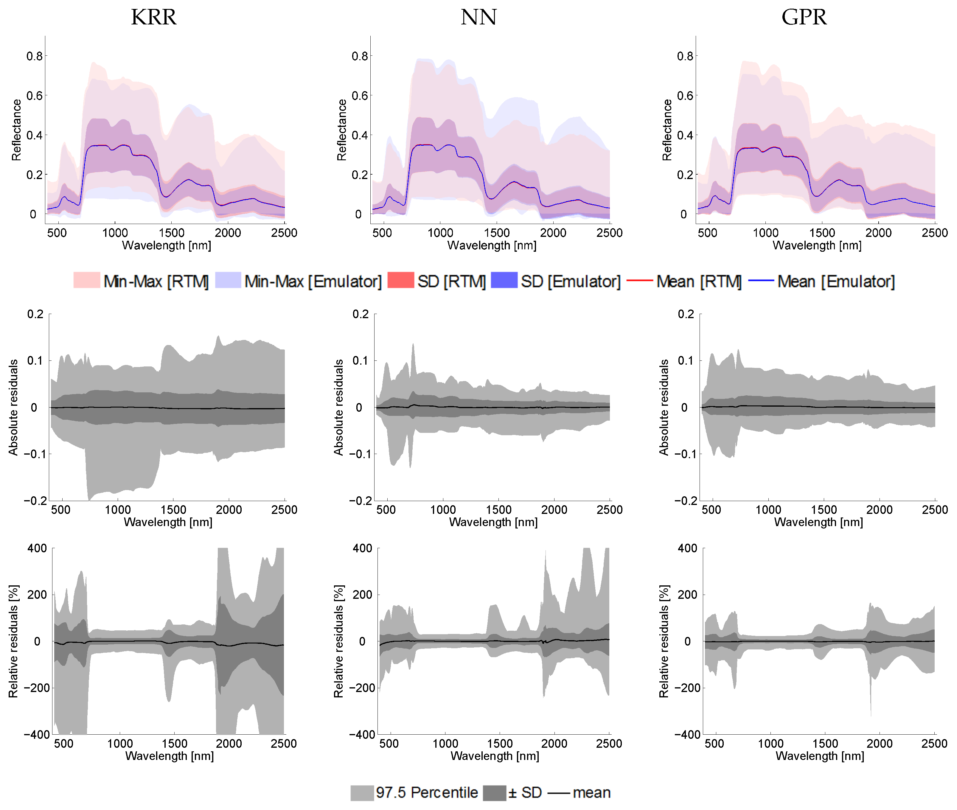
6.2.2. PROSAIL
6.2.3. MODTRAN5
6.3. Global Sensitivity Analysis Results
6.3.1. PROSPECT-4
6.3.2. PROSAIL
6.3.3. MODTRAN5
7. Discussion
7.1. Interpreting Emulator Results
7.2. Interpreting Sensitivity Analysis Results
7.3. New Processing Opportunities with Emulators
8. Conclusions
Acknowledgments
Author Contributions
Conflicts of Interest
References
- Zhang, Y.; Rossow, W.; Lacis, A.; Oinas, V.; Mishchenko, M. Calculation of radiative fluxes from the surface to top of atmosphere based on ISCCP and other global data sets: Refinements of the radiative transfer model and the input data. J. Geophys. Res. D Atmos. 2004, 109. [Google Scholar] [CrossRef]
- Jacquemoud, S.; Verhoef, W.; Baret, F.; Bacour, C.; Zarco-Tejada, P.; Asner, G.; François, C.; Ustin, S. PROSPECT + SAIL models: A review of use for vegetation characterization. Remote Sens. Environ. 2009, 113, S56–S66. [Google Scholar] [CrossRef]
- Deiveegan, M.; Balaji, C.; Venkateshan, S. A polarized microwave radiative transfer model for passive remote sensing. Atmos. Res. 2008, 88, 277–293. [Google Scholar] [CrossRef]
- Van der Tol, C.; Berry, J.A.; Campbell, P.K.E.; Rascher, U. Models of fluorescence and photosynthesis for interpreting measurements of solar-induced chlorophyll fluorescence. J. Geophys. Res. Biogeosci. 2014, 119, 2312–2327. [Google Scholar] [CrossRef] [PubMed]
- Verrelst, J.; Camps-Valls, G.; Muñoz-Marí, J.; Rivera, J.; Veroustraete, F.; Clevers, J.; Moreno, J. Optical remote sensing and the retrieval of terrestrial vegetation bio-geophysical properties—A review. ISPRS J. Photogramm. Remote Sens. 2015, 108, 273–290. [Google Scholar] [CrossRef]
- Verhoef, W.; Bach, H. Simulation of Sentinel-3 images by four-stream surface-atmosphere radiative transfer modeling in the optical and thermal domains. Remote Sens. Environ. 2012, 120, 197–207. [Google Scholar] [CrossRef]
- Meharrar, K.; Bachari, N. Modelling of radiative transfer of natural surfaces in the solar radiation spectrum: Development of a satellite data simulator (SDDS). Int. J. Remote Sens. 2014, 35, 1199–1216. [Google Scholar] [CrossRef]
- Segl, K.; Guanter, L.; Rogass, C.; Kuester, T.; Roessner, S.; Kaufmann, H.; Sang, B.; Mogulsky, V.; Hofer, S. EeteSThe EnMAP end–to–end simulation tool. IEEE J. Sel. Top. Appl. Earth Obs. Remote Sens. 2012, 5, 522–530. [Google Scholar] [CrossRef]
- Vicent, J.; Sabater, N.; Tenjo, C.; Acarreta, J.; Manzano, M.; Rivera, J.; Jurado, P.; Franco, R.; Alonso, L.; Verrelst, J.; et al. FLEX End-to-End Mission Performance Simulator. IEEE Trans. Geosci. Remote Sens. 2016, 54, 4215–4223. [Google Scholar] [CrossRef]
- Widlowski, J.L.; Taberner, M.; Pinty, B.; Bruniquel-Pinel, V.; Disney, M.; Fernandes, R.; Gastellu-Etchegorry, J.P.; Gobron, N.; Kuusk, A.; Lavergne, T.; et al. Third Radiation Transfer Model Intercomparison (RAMI) exercise: Documenting progress in canopy reflectance models. J. Geophys. Res. Atmos. 2007, 112. [Google Scholar] [CrossRef] [Green Version]
- Baret, F.; Buis, S. Estimating canopy characteristics from remote sensing observations. Review of methods and associated problems. In Advances in Land Remote Sensing: System, Modeling, Inversion and Application; Liang, S., Ed.; Springer: Berlin/Heidelberg, Germany, 2008; pp. 171–200. [Google Scholar]
- Widlowski, J.L.; Pinty, B.; Lopatka, M.; Atzberger, C.; Buzica, D.; Chelle, M.; Disney, M.; Gastellu-Etchegorry, J.P.; Gerboles, M.; Gobron, N.; et al. The fourth radiation transfer model intercomparison (RAMI-IV): Proficiency testing of canopy reflectance models with ISO-13528. J. Geophys. Res. Atmos. 2013, 118, 6869–6890. [Google Scholar] [CrossRef]
- Widlowski, J.L.; Mio, C.; Disney, M.; Adams, J.; Andredakis, I.; Atzberger, C.; Brennan, J.; Busetto, L.; Chelle, M.; Ceccherini, G.; et al. The fourth phase of the radiative transfer model intercomparison (RAMI) exercise: Actual canopy scenarios and conformity testing. Remote Sens. Environ. 2015, 169, 418–437. [Google Scholar] [CrossRef]
- Feret, J.B.; François, C.; Asner, G.P.; Gitelson, A.A.; Martin, R.E.; Bidel, L.P.R.; Ustin, S.L.; le Maire, G.; Jacquemoud, S. PROSPECT-4 and 5: Advances in the leaf optical properties model separating photosynthetic pigments. Remote Sens. Environ. 2008, 112, 3030–3043. [Google Scholar] [CrossRef]
- Verhoef, W. Light scattering by leaf layers with application to canopy reflectance modeling: The SAIL model. Remote Sens. Environ. 1984, 16, 125–141. [Google Scholar] [CrossRef]
- Vermote, E.; Tanré, D.; Deuzé, J.; Herman, M.; Morcrette, J.J. Second simulation of the satellite signal in the solar spectrum, 6S: An overview. IEEE Trans. Geosci. Remote Sens. 1997, 35, 675–686. [Google Scholar] [CrossRef]
- Lipton, A.; Moncet, J.L.; Boukabara, S.A.; Uymin, G.; Quinn, K. Fast and accurate radiative transfer in the microwave with optimum spectral sampling. IEEE Trans. Geosci. Remote Sens. 2009, 47, 1909–1917. [Google Scholar] [CrossRef]
- Govaerts, Y.M.; Verstraete, M.M. Raytran: A Monte Carlo ray-tracing model to compute light scattering in three-dimensional heterogeneous media. IEEE Trans. Geosci. Remote Sens. 1998, 36, 493–505. [Google Scholar] [CrossRef]
- North, P. Three-dimensional forest light interaction model using a Monte Carlo method. IEEE Trans. Geosci. Remote Sens. 1996, 34, 946–956. [Google Scholar] [CrossRef]
- Lewis, P. Three-dimensional plant modelling for remote sensing simulation studies using the Botanical Plant Modelling System. Agronomie 1999, 19, 185–210. [Google Scholar] [CrossRef]
- Gastellu-Etchegorry, J.; Demarez, V.; Pinel, V.; Zagolski, F. Modeling radiative transfer in heterogeneous 3-D vegetation canopies. Remote Sens. Environ. 1996, 58, 131–156. [Google Scholar] [CrossRef]
- Petropoulos, G.; Wooster, M.; Carlson, T.; Kennedy, M.; Scholze, M. A global Bayesian sensitivity analysis of the 1D SimSphere soil vegetation atmospheric transfer (SVAT) model using Gaussian model emulation. Ecol. Model. 2009, 220, 2427–2440. [Google Scholar] [CrossRef]
- Van Der Tol, C.; Verhoef, W.; Timmermans, J.; Verhoef, A.; Su, Z. An integrated model of soil-canopy spectral radiances, photosynthesis, fluorescence, temperature and energy balance. Biogeosciences 2009, 6, 3109–3129. [Google Scholar] [CrossRef]
- Berk, A.; Anderson, G.; Acharya, P.; Bernstein, L.; Muratov, L.; Lee, J.; Fox, M.; Adler-Golden, S.; Chetwynd, J.; Hoke, M.; et al. MODTRANTM5: 2006 update. In Proceedings of the Algorithms and Technologies for Multispectral, Hyperspectral, and Ultraspectral Imagery XII, Orlando, FL, USA, 17 April 2006; Volume 6233.
- España, M.; Baret, F.; Aries, F.; Chelle, M.; Andrieu, B.; Prévot, L. Modeling maize canopy 3D architecture: Application to reflectance simulation. Ecol. Model. 1999, 122, 25–43. [Google Scholar] [CrossRef]
- Mousivand, A.; Menenti, M.; Gorte, B.; Verhoef, W. Multi-temporal, multi-sensor retrieval of terrestrial vegetation properties from spectral-directional radiometric data. Remote Sens. Environ. 2015, 158, 311–330. [Google Scholar] [CrossRef]
- Saltelli, A.; Ratto, M.; Andres, T.; Campolongo, F.; Cariboni, J.; Gatelli, D.; Saisana, M.; Tarantola, S. Global Sensitivity Analysis: The Primer; John Wiley & Sons: Hoboken, NJ, USA, 2008. [Google Scholar]
- Yang, J. Convergence and uncertainty analyses in Monte-Carlo based sensitivity analysis. Environ. Model. Softw. 2011, 26, 444–457. [Google Scholar] [CrossRef]
- Nossent, J.; Elsen, P.; Bauwens, W. Sobol’sensitivity analysis of a complex environmental model. Environ. Model. Softw. 2011, 26, 1515–1525. [Google Scholar] [CrossRef]
- Bowyer, P.; Danson, F. Sensitivity of spectral reflectance to variation in live fuel moisture content at leaf and canopy level. Remote Sens. Environ. 2004, 92, 297–308. [Google Scholar] [CrossRef]
- Stuckens, J.; Verstraeten, W.W.; Delalieux, S.; Swennen, R.; Coppin, P. A dorsiventral leaf radiative transfer model: Development, validation and improved model inversion techniques. Remote Sens. Environ. 2009, 113, 2560–2573. [Google Scholar] [CrossRef]
- Mousivand, A.; Menenti, M.; Gorte, B.; Verhoef, W. Global sensitivity analysis of the spectral radiance of a soil–vegetation system. Remote Sens. Environ. 2014, 145, 131–144. [Google Scholar] [CrossRef]
- Verrelst, J.; Rivera, J.; Van Der Tol, C.; Magnani, F.; Mohammed, G.; Moreno, J. Global sensitivity analysis of the SCOPE model: What drives simulated canopy-leaving sun-induced fluorescence? Remote Sens. Environ. 2015, 166, 8–21. [Google Scholar] [CrossRef]
- O’Hagan, A. Bayesian analysis of computer code outputs: A tutorial. Reliab. Eng. Syst. Saf. 2006, 91, 1290–1300. [Google Scholar] [CrossRef]
- Rohmer, J.; Foerster, E. Global sensitivity analysis of large-scale numerical landslide models based on Gaussian-Process meta-modeling. Comput. Geosci. 2011, 37, 917–927. [Google Scholar] [CrossRef]
- Bounceur, N.; Crucifix, M.; Wilkinson, R. Global sensitivity analysis of the climate–vegetation system to astronomical forcing: An emulator-based approach. Earth Syst. Dyn. Discuss. 2014, 5, 901–943. [Google Scholar] [CrossRef]
- Rivera, J.P.; Verrelst, J.; Gómez-Dans, J.; Muñoz Marí, J.; Moreno, J.; Camps-Valls, G. An Emulator Toolbox to Approximate Radiative Transfer Models with Statistical Learning. Remote Sens. 2015, 7, 9347. [Google Scholar] [CrossRef]
- Gómez-Dans, J.L.; Lewis, P.E.; Disney, M. Efficient Emulation of Radiative Transfer Codes Using Gaussian Processes and Application to Land Surface Parameter Inferences. Remote Sens. 2016, 8, 119. [Google Scholar] [CrossRef]
- Carnevale, C.; Finzi, G.; Guariso, G.; Pisoni, E.; Volta, M. Surrogate models to compute optimal air quality planning policies at a regional scale. Environ. Model. Softw. 2012, 34, 44–50. [Google Scholar] [CrossRef]
- Villa-Vialaneix, N.; Follador, M.; Ratto, M.; Leip, A. A comparison of eight metamodeling techniques for the simulation of N2O fluxes and N leaching from corn crops. Environ. Model. Softw. 2012, 34, 51–66. [Google Scholar] [CrossRef] [Green Version]
- Castelletti, A.; Galelli, S.; Ratto, M.; Soncini-Sessa, R.; Young, P. A general framework for dynamic emulation modelling in environmental problems. Environ. Model. Softw. 2012, 34, 5–18. [Google Scholar] [CrossRef]
- Lee, L.; Pringle, K.; Reddington, C.; Mann, G.; Stier, P.; Spracklen, D.; Pierce, J.; Carslaw, K. The magnitude and causes of uncertainty in global model simulations of cloud condensation nuclei. Atmos. Chem. Phys. 2013, 13, 8879–8914. [Google Scholar] [CrossRef]
- Ireland, G.; Petropoulos, G.; Carlson, T.; Purdy, S. Addressing the ability of a land biosphere model to predict key biophysical vegetation characterisation parameters with Global Sensitivity Analysis. Environ. Model. Softw. 2015, 65, 94–107. [Google Scholar] [CrossRef]
- Camps-Valls, G.; Bruzzone, L. (Eds.) Kernel Methods for Remote Sensing Data Analysis; Wiley & Sons Ltd.: Chichester, UK, 2009.
- Razavi, S.; Tolson, B.A.; Burn, D.H. Numerical assessment of metamodelling strategies in computationally intensive optimization. Environ. Model. Softw. 2012, 34, 67–86. [Google Scholar] [CrossRef]
- Verrelst, J.; Muñoz, J.; Alonso, L.; Delegido, J.; Rivera, J.; Camps-Valls, G.; Moreno, J. Machine learning regression algorithms for biophysical parameter retrieval: Opportunities for Sentinel-2 and -3. Remote Sens. Environ. 2012, 118, 127–139. [Google Scholar] [CrossRef]
- Rivera, J.; Verrelst, J.; Delegido, J.; Veroustraete, F.; Moreno, J. On the semi-automatic retrieval of biophysical parameters based on spectral index optimization. Remote Sens. 2014, 6, 4924–4951. [Google Scholar] [CrossRef]
- Wold, S.; Esbensen, K.; Geladi, P. Principal component analysis. Chemom. Intell. Lab. Syst. 1987, 2, 37–52. [Google Scholar] [CrossRef]
- Camps-Valls, G.; Muñoz-Marí, J.; Gómez-Chova, L.; Guanter, L.; Calbet, X. Nonlinear statistical retrieval of atmospheric profiles from MetOp-IASI and MTG-IRS infrared sounding data. IEEE Trans. Geosci. Remote Sens. 2012, 50, 1759–1769. [Google Scholar] [CrossRef]
- Camps-Valls, G.; Verrelst, J.; Muñoz-Marí, J.; Laparra, V.; Mateo-Jiménez, F.; Gómez-Dans, J. A Survey on Gaussian Processes for Earth Observation Data Analysis. IEEE Geosci. Remote Sens. Mag. 2016, 4, 58–78. [Google Scholar] [CrossRef]
- Camps-Valls, G.; Gómez-Chova, L.; Muñoz-Marí, J.; Lázaro-Gredilla, M.; Verrelst, J. SimpleR: A Simple Educational Matlab Toolbox for Statistical Regression, 2013. Available online: http://isp.uv.es/softregression.html (accessed on 18 August 2016).
- Sobol’, I.M. On sensitivity estimation for nonlinear mathematical models. Mat. Model. 1990, 2, 112–118. [Google Scholar]
- McRae, G.J.; Tilden, J.W.; Seinfeld, J.H. Global sensitivity analysis—A computational implementation of the Fourier amplitude sensitivity test (FAST). Comput. Chem. Eng. 1982, 6, 15–25. [Google Scholar] [CrossRef]
- Saltelli, A.; Annoni, P.; Azzini, I.; Campolongo, F.; Ratto, M.; Tarantola, S. Variance based sensitivity analysis of model output. Design and estimator for the total sensitivity index. Comput. Phys. Commun. 2010, 181, 259–270. [Google Scholar] [CrossRef]
- Song, X.; Bryan, B.A.; Paul, K.I.; Zhao, G. Variance-based sensitivity analysis of a forest growth model. Ecol. Model. 2012, 247, 135–143. [Google Scholar] [CrossRef]
- Saltelli, A.; Annoni, P. How to avoid a perfunctory sensitivity analysis. Environ. Model. Softw. 2010, 25, 1508–1517. [Google Scholar] [CrossRef]
- Saltelli, A. Making best use of model evaluations to compute sensitivity indices. Comput. Phys. Commun. 2002, 145, 280–297. [Google Scholar] [CrossRef]
- Verhoef, W.; Jia, L.; Xiao, Q.; Su, Z. Unified optical-thermal four-stream radiative transfer theory for homogeneous vegetation canopies. IEEE Trans. Geosci. Remote Sens. 2007, 45, 1808–1822. [Google Scholar] [CrossRef]
- Wang, P.; Liu, K.Y.; Cwik, T.; Green, R. MODTRAN on supercomputers and parallel computers. Parallel Comput. 2002, 28, 53–64. [Google Scholar] [CrossRef]
- Stamnes, K.; Tsay, S.C.; Wiscombe, W.; Jayaweera, K. Numerically stable algorithm for discrete-ordinate-method radiative transfer in multiple scattering and emitting layered media. Appl. Opt. 1988, 27, 2502–2509. [Google Scholar] [CrossRef] [PubMed]
- Goody, R.; West, R.; Chen, L.; Crisp, D. The correlated-k method for radiation calculations in nonhomogeneous atmospheres. J. Quant. Spectrosc. Radiat. Transf. 1989, 42, 539–550. [Google Scholar] [CrossRef]
- Berk, A.; Anderson, G.; Acharya, P.; Shettle, E. MODTRAN 5.2.1 User’s Manual; Spectral Science Inc.: Burlingtonm, MA, USA, 2011. [Google Scholar]
- Guanter, L.; Richter, R.; Kaufmann, H. On the application of the MODTRAN4 atmospheric radiative transfer code to optical Remote Sensing. Int. J. Remote Sens. 2009, 30, 1407–1424. [Google Scholar] [CrossRef]
- Richter, R.; Schläpfer, D. Geo-atmospheric processing of airborne imaging spectrometry data. Part 2: Atmospheric/topographic correction. Int. J. Remote Sens. 2002, 23, 2631–2649. [Google Scholar] [CrossRef]
- Cooley, T.; Anderson, G.; Felde, G.; Hoke, M.; Ratkowski, A.; Chetwynd, J.; Gardner, J.; Adler-Golden, S.; Matthew, M.; Berk, A.; et al. FLAASH, a MODTRAN4-based atmospheric correction algorithm, its applications and validation. In IEEE International Geoscience and Remote Sensing Symposium; IEEE: Piscataway, NJ, USA, 2002; Volume 3, pp. 1414–1418. [Google Scholar]
- Guanter, L. New Algorithms for Atmospheric Correction and Retrieval of Biophysical Parameters in Earth Observation: Application to ENVISAT/MERIS Data, 2006. Available online: http://hdl.handle.net/10803/9877 (accessed on 18 August 2016).
- Berk, A.; Acharya, P.; Anderson, G.; Gossage, B. Recent developments in the MODTRAN atmospheric model and implications for hyperspectral compensation. In 2009 IEEE International Geoscience and Remote Sensing Symposium; IEEE: Piscataway, NJ, USA, 2009; Volume 2, pp. II262–II265. [Google Scholar]
- Verrelst, J.; Romijn, E.; Kooistra, L. Mapping vegetation density in a heterogeneous river floodplain ecosystem using pointable CHRIS/PROBA data. Remote Sens. 2012, 4, 2866–2889. [Google Scholar] [CrossRef]
- Verrelst, J.; Rivera, J.; Moreno, J. ARTMO’s Global Sensitivity Analysis (GSA) toolbox to quantify driving variables of leaf and canopy radiative transfer models. EARSeL eProc. 2015, 14, 1–11. [Google Scholar]
- McKay, M.; Beckman, R.; Conover, W. Comparison of three methods for selecting values of input variables in the analysis of output from a computer code. Technometrics 1979, 21, 239–245. [Google Scholar]
- Conti, S.; O’Hagan, A. Bayesian emulation of complex multi-output and dynamic computer models. J. Stat. Plan. Inference 2010, 140, 640–651. [Google Scholar] [CrossRef]
- Kennedy, M.; O’Hagan, A. Bayesian calibration of computer models. J. R. Stat. Soc. Ser. B Stat. Methodol. 2001, 63, 425–450. [Google Scholar] [CrossRef]
- Hankin, R.K. Introducing BACCO, an R package for Bayesian analysis of computer code output. J. Stat. Softw. 2005, 14, 1–21. [Google Scholar] [CrossRef]
- Conti, S.; Gosling, J.; Oakley, J.; O’Hagan, A. Gaussian process emulation of dynamic computer codes. Biometrika 2009, 96, 663–676. [Google Scholar] [CrossRef]
- Verrelst, J.; Alonso, L.; Camps-Valls, G.; Delegido, J.; Moreno, J. Retrieval of vegetation biophysical parameters using Gaussian process techniques. IEEE Trans. Geosci. Remote Sens. 2012, 50, 1832–1843. [Google Scholar] [CrossRef]
- Verrelst, J.; Rivera, J.; Moreno, J.; Camps-Valls, G. Gaussian processes uncertainty estimates in experimental Sentinel-2 LAI and leaf chlorophyll content retrieval. ISPRS J. Photogramm. Remote Sens. 2013, 86, 157–167. [Google Scholar] [CrossRef]
- Hansen, J.E.; Travis, L.D. Light scattering in planetary atmospheres. Space Sci. Rev. 1974, 16, 527–610. [Google Scholar] [CrossRef]
- Verrelst, J.; van der Tol, C.; Magnani, F.; Sabater, N.; Rivera, J.; Mohammed, G.; Moreno, J. Evaluating the predictive power of sun-induced chlorophyll fluorescence to estimate net photosynthesis of vegetation canopies: A SCOPE modeling study. Remote Sens. Environ. 2016, 176, 139–151. [Google Scholar] [CrossRef]
- Ollinger, S. Sources of variability in canopy reflectance and the convergent properties of plants. New Phytol. 2011, 189, 375–394. [Google Scholar] [CrossRef] [PubMed]
- Jacquemoud, S.; Baret, F.; Andrieu, B.; Danson, F.; Jaggard, K. Extraction of vegetation biophysical parameters by inversion of the PROSPECT + SAIL models on sugar beet canopy reflectance data. Application to TM and AVIRIS sensors. Remote Sens. Environ. 1995, 52, 163–172. [Google Scholar] [CrossRef]
- Kuusk, A. Monitoring of vegetation parameters on large areas by the inversion of a canopy reflectance model. Int. J. Remote Sens. 1998, 19, 2893–2905. [Google Scholar] [CrossRef]
- Myneni, R.; Hoffman, S.; Knyazikhin, Y.; Privette, J.; Glassy, J.; Tian, Y.; Wang, Y.; Song, X.; Zhang, Y.; Smith, G.; et al. Global products of vegetation leaf area and fraction absorbed PAR from year one of MODIS data. Remote Sens. Environ. 2002, 83, 214–231. [Google Scholar] [CrossRef]
- Richter, R. A spatially adaptive fast atmospheric correction algorithm. Int. J. Remote Sens. 1996, 17, 1201–1214. [Google Scholar] [CrossRef]
- Thome, K.; Palluconi, F.; Takashima, T.; Masuda, K. Atmospheric correction of ASTER. IEEE Trans. Geosci. Remote Sens. 1998, 36, 1199–1211. [Google Scholar] [CrossRef]
- Kotchenova, S.; Vermote, E.; Matarrese, R.; Klemm, F., Jr. Validation of a vector version of the 6S radiative transfer code for atmospheric correction of satellite data. Part I: Path radiance. Appl. Opt. 2006, 45, 6762–6774. [Google Scholar] [CrossRef] [PubMed]
- Guanter, L.; Alonso, L.; Moreno, J. CHRIS Proba Atmospheric Correction Module. Available online: http://www.brockmann-consult.de/beam-wiki/download/attachments/32964611/chrisbox-atmosphericcorrectionatbd-2.0.pdf (accessed on 2 June 2012).
- Hagolle, O.; Huc, M.; Pascual, D.; Dedieu, G. A multi-temporal and multi-spectral method to estimate aerosol optical thickness over land, for the atmospheric correction of FormoSat-2, LandSat, VENμS and Sentinel-2 images. Remote Sens. 2015, 7, 2668–2691. [Google Scholar] [CrossRef]
- Segl, K.; Guanter, L.; Gascon, F.; Kuester, T.; Rogass, C.; Mielke, C. S2eteS: An End-to-End Modeling Tool for the Simulation of Sentinel-2 Image Products. IEEE Trans. Geosci. Remote. Sens. 2015, 53, 5560–5571. [Google Scholar] [CrossRef]
- Rivera, J.; Sabater, N.; Tenjo, C.; Vicent, J.; Moreno, J. Synthetic scene simulator for hyperspectral spaceborne passive optical sensors. Application to ESA’s FLEX/Sentinel-3 tandem mission. In Proceedings of the WHISPERS—6th Workshop on Hyperspectral Image and Signal: Evolution in Remote Sensing, Lausanne, Switzerland, 24–27 June 2014.
- Quaife, T.; Lewis, P.; De Kauwe, M.; Williams, M.; Law, B.; Disney, M.; Bowyer, P. Assimilating canopy reflectance data into an ecosystem model with an Ensemble Kalman Filter. Remote Sens. Environ. 2008, 112, 1347–1364. [Google Scholar] [CrossRef]
- Peng, C.; Guiot, J.; Wu, H.; Jiang, H.; Luo, Y. Integrating models with data in ecology and palaeoecology: Advances towards a model-data fusion approach. Ecol. Lett. 2011, 14, 522–536. [Google Scholar] [CrossRef] [PubMed]
- Luo, Y.; Ogle, K.; Tucker, C.; Fei, S.; Gao, C.; LaDeau, S.; Clark, J.; Schimel, D. Ecological forecasting and data assimilation in a data-rich era. Ecol. Appl. 2011, 21, 1429–1442. [Google Scholar] [CrossRef] [PubMed]
- Lewis, P.; Gómez-Dans, J.; Kaminski, T.; Settle, J.; Quaife, T.; Gobron, N.; Styles, J.; Berger, M. An Earth Observation Land Data Assimilation System (EO-LDAS). Remote Sens. Environ. 2012, 120, 219–235. [Google Scholar] [CrossRef]
- Salcedo-Sanz, S.; Casanova-Mateo, C.; Muñoz Marí, J.; Camps-Valls, G. Prediction of daily global solar irradiation using temporal Gaussian processes. IEEE Geosci. Remote Sens. Lett. 2014, 11, 1936–1940. [Google Scholar] [CrossRef]
- Arenas-García, J.; Petersen, K.B.; Camps-Valls, G.; Hansen, L.K. Kernel Multivariate Analysis Framework for Supervised Subspace Learning. IEEE Signal Process. Mag. 2013, 30, 16–29. [Google Scholar] [CrossRef]
- Camps-Valls, G.; Jung, M.; Ichii, K.; Papale, D.; Tramontana, G.; Bodesheim, P.; Schwalm, C.; Zscheischler, J.; Mahecha, M.; Reichstein, M. Ranking drivers of global carbon and energy fluxes over land. In Proceedings of the 2015 IEEE International Geoscience and Remote Sensing Symposium (IGARSS), Milan, Italy, 26–31 July 2015; pp. 4416–4419.
- Oakley, J.; O’Hagan, A. Probabilistic sensitivity analysis of complex models: A Bayesian approach. J. R. Stat. Soc. Ser. B Stat. Methodol. 2004, 66, 751–769. [Google Scholar] [CrossRef]


| Model Variales | Units | Minimum | Maximum | |
|---|---|---|---|---|
| Leaf variables: PROSPECT-4 | ||||
| N | Leaf structure index | unitless | 1.0 | 4.0 |
| Leaf water content | cm | 0.001 | 0.05 | |
| Leaf chlorophyll content | g/cm | 0.1 | 100 | |
| Leaf dry matter content | g/cm | 0.001 | 0.05 | |
| Canopy variables: SAIL | ||||
| Leaf area index | m/m | 0.1 | 10 | |
| Average leaf angle | ∘ | 0 | 90 | |
| Diffuse incoming solar radiation | fraction | 0 | 100 | |
| Soil scaling factor | unitless | 0 | 1 | |
| Sun zenith angle | ∘ | 0 | 60 | |
| View zenith angle | ∘ | 0 | 55 | |
| (Sun-sensor) relative azimuth angle | ∘ | 0 | 180 | |
| Atmospheric variables: MODTRAN5 | ||||
| Visual zenith angle | ∘ | 0 | 55 | |
| Solar zenith angle | ∘ | 0 | 60 | |
| Relative azimuth angle | ∘ | 0 | 180 | |
| Elevation | km | 0 | 2 | |
| Aerosol optical thickness | - | 0 | 0.4 | |
| Angstrom Coefficient | - | 0.5 | 3 | |
| G | Asymmetry parameter | - | −1 | 1 |
| Columnar water vapor | g/cm | 0 | 2 | |
| MLRA | RMSE | NRMSE (%) | CPU (s) |
|---|---|---|---|
| PROSPECT-4 | |||
| KRR | 0.19 | 0.03 | 1 |
| NN | 0.08 | 0.01 | 730 |
| GPR | 0.16 | 0.01 | 90 |
| PROSAIL | |||
| KRR | 1.79 | 0.24 | 1 |
| NN | 0.85 | 0.11 | 208 |
| GPR | 0.90 | 0.11 | 100 |
| MODTRAN5 | |||
| KRR | 403.55 | 0.05 | 1 |
| NN | 1137.30 | 0.12 | 157 |
| GPR | 263.54 | 0.03 | 82 |
| MODTRAN5 | |||
| KRR | 738.47 | 0.04 | 1 |
| NN | 3117.30 | 0.18 | 878 |
| GPR | 1372.90 | 0.08 | 123 |
| MODTRAN5 | |||
| KRR | 0.53 | 0.07 | 1 |
| NN | 0.24 | 0.04 | 321 |
| GPR | 0.25 | 0.04 | 80 |
| MODTRAN5 | |||
| KRR | 1.11 | 0.07 | 1 |
| NN | 0.34 | 0.05 | 280 |
| GPR | 0.48 | 0.03 | 80 |
| MODTRAN5 S | |||
| KRR | 0.29 | 0.04 | 1 |
| NN | 0.21 | 0.03 | 271 |
| GPR | 0.30 | 0.04 | 78 |
| MODTRAN5 | |||
| KRR | 1489.90 | 0.14 | 1 |
| NN | 1086.40 | 0.43 | 186 |
| GPR | 729.10 | 0.07 | 94 |
© 2016 by the authors; licensee MDPI, Basel, Switzerland. This article is an open access article distributed under the terms and conditions of the Creative Commons Attribution (CC-BY) license (http://creativecommons.org/licenses/by/4.0/).
Share and Cite
Verrelst, J.; Sabater, N.; Rivera, J.P.; Muñoz-Marí, J.; Vicent, J.; Camps-Valls, G.; Moreno, J. Emulation of Leaf, Canopy and Atmosphere Radiative Transfer Models for Fast Global Sensitivity Analysis. Remote Sens. 2016, 8, 673. https://doi.org/10.3390/rs8080673
Verrelst J, Sabater N, Rivera JP, Muñoz-Marí J, Vicent J, Camps-Valls G, Moreno J. Emulation of Leaf, Canopy and Atmosphere Radiative Transfer Models for Fast Global Sensitivity Analysis. Remote Sensing. 2016; 8(8):673. https://doi.org/10.3390/rs8080673
Chicago/Turabian StyleVerrelst, Jochem, Neus Sabater, Juan Pablo Rivera, Jordi Muñoz-Marí, Jorge Vicent, Gustau Camps-Valls, and José Moreno. 2016. "Emulation of Leaf, Canopy and Atmosphere Radiative Transfer Models for Fast Global Sensitivity Analysis" Remote Sensing 8, no. 8: 673. https://doi.org/10.3390/rs8080673