Estimating Savanna Clumping Index Using Hemispherical Photographs Integrated with High Resolution Remote Sensing Images

Abstract

In contrast to herbaceous canopies and forests, savannas are grassland ecosystems with sparsely distributed individual trees, so the canopy is spatially heterogeneous and open, whereas the woody cover in savannas, e.g., tree cover, adversely affects ecosystem structures and functions. Studies have shown that the dynamics of canopy structure are related to available water, climate, and human activities in the form of porosity, leaf area index (LAI), and clumping index (CI). Therefore, it is important to identify the biophysical parameters of savanna ecosystems, and undertake practical actions for savanna conservation and management. The canopy openness presents a challenge for evaluating canopy LAI and other biophysical parameters, as most remotely sensed methods were developed for homogeneous and closed canopies. Clumping index is a key variable that can represent the clumping effect from spatial distribution patterns of components within a canopy. However, it is a difficult task to measure the clumping index of the moderate resolution savanna pixels directly using optical instruments, such as the Tracing Radiation and Architecture of Canopies, LAI-2000 Canopy Analyzer, or digital hemispherical photography. This paper proposed a new method using hemispherical photographs combined with high resolution remote sensing images to estimate the clumping index of savanna canopies. The effects of single tree LAI, crown density, and herbaceous layer on the clumping index of savanna pixels were also evaluated. The proposed method effectively calculated the clumping index of moderate resolution pixels. The clumping indices of two study regions located in Ejina Banner and Weichang were compared with the clumping index product over China’s landmass.

1. Introduction

Earth surface vegetation presents various canopy morphologies [1]. In contrast to herbaceous canopies and forests, savannas are grassland ecosystems with sparsely distributed individual trees, so the canopy does not close [2,3]. The open canopy allows sufficient light to reach the ground to support an unbroken herbaceous layer consisting primarily of grasses [4,5]. Savannas are always located in water limited regions where potential evaporation exceeds precipitation, and cover approximately 20% of Earth’s land area [6,7,8]. Hence, they are anticipated to be among the ecosystems most sensitive to future land use and climate changes [9,10], and it is important to gain a mechanistic understanding of their vegetation–atmosphere exchange. While the woody cover in savannas, e.g., tree cover, adversely affect ecosystem structures and functions, an intensive understanding of woody cover is required for savanna conservation and management [11]. Woody cover growth is related to available water, climate, human activities [12], and herbivory level [11] in the form of porosity, leaf area index (LAI), and clumping index (CI). Savannas are spatially heterogeneous, open ecosystems, and the canopy openness presents a challenge for evaluating canopy LAI and other biophysical parameters, since most remotely sensed methods were developed for ideal and closed canopies [13,14]. CI is a key variable that can represent clumping effects caused by spatial distribution patterns of components within the canopy [15]. Chen et al. [16] also demonstrated the importance of CI for LAI estimation and carbon cycle modeling, since it allows a better segmentation of the solar radiation distribution in sunlit and shaded leaves as compared to models that relate carbon absorption only to the intercepted solar radiation. Therefore, CI is a very important parameter to describe spatial heterogeneity and clumping effects of savanna canopies.

The Poisson model [17] has been widely used to calculate porosity and estimate LAI when leaves are randomly distributed within canopies. For the case of non-random distribution of vegetation elements, the elements would be disparate at different scales, such as at shoot levels [18,19,20,21], among canopies levels [22,23], and at ecosystem level (such as savannas) [14,24]. The confined distribution of foliage in these structures is referred to as clumping [25], and ignoring clumping leads to increased gap fractions and LAI underestimation using a simple random model [26]. Nilson [17] introduced CI (foliage dispersion parameter) to describe clumping effects and correct the Poisson model. Studies have shown that the bidirectional transmittance of non-random vegetation canopy can be better described using the modified Poisson model [6,17,25,27,28]. Accordingly, the gap probability should be the key to retrieve CI using the modified Poisson model.

Some research on retrieving CI has been based on satellite remote sensing data. Global mapping of foliage clumping index has been derived using Polarization and Direction of Earth’s Reflectance (POLDER) 1, POLDER 3 and Moderate Resolution Imaging Spectrometer (MODIS) data based on reflectance of hotspots and darkspots [15,29,30]. Pisek et al. [31] compared CI estimates among POLDER, MODIS, and Multi-angle Imaging SpectroRadiometer (MISR) satellite remote sensing date. Zhu et al. [32] and He et al. [33] also estimated CI over China’s landmass using the MODIS bidirectional reflectance distribution function (BDRF) data based on the normalized difference between hotspot and darkspot (NDHD) method. He et al. [34] also analyzed inter and intra-annual CI variations derived from MODIS BRDF product based on NDHD. For savanna canopy, pixel reflectance was contributed by both unbroken herbaceous layer and tree cover. For more homogeneous forest, background reflectance was retrieved from MISR data [35] and compact airborne spectrographic imager (CASI) data [36]. The influence was incorporated in the LAI algorithm [37]. Olofsson and Eklundh [38] found retrieved FAPAR were strongly different from measured values for sparse canopies, since the understory vegetation of sparse stands contributed to the total absorption and affected the reflectance. Therefore, following the definition of CI, the effects of herbaceous layers should be considered.

Clumping index true value can also be obtained through ground measurements in situ. It has usually been acquired using optical instruments, such as the Tracing Radiation and Architecture of Canopies (TRAC), LAI-2000 canopy analyzer, and digital hemispherical photography. Chen [19] and Chen et al. [39] derived the CI of boreal forest using gap size distributions [18] with TRAC. Chianucci et al. [40] estimated foliage clumping from the LAI-2000 plant canopy analyzer based on a logarithmic averaging method. Van Gardingen et al. [41] used the Lang and Xiang finite length averaging method to measure the CI with hemispherical photographs. Walter et al. [42] used a gap size accumulation method [18] and the Pielou coefficient of spatial segregation to extract CI from film-based hemispherical photographs. Demarez et al. [43] calculated the gap fraction and retrieved the CI for row crops utilizing hemispherical photographs. Chianucci and Cutini [44], Pekin and Macfarlane [45], Gonsamo and Pellikka [26] estimated CI for forests using digital hemispherical photography. Kucharik et al. [22,46] used a multiband vegetation imager (MVI) to measure gap fraction and gap size distribution to calculate the zenith CI. Zhao et al. [47] estimated CI for forests using a full-waveform ground based lidar. Although these methods can be adapted to continuous forests with lower openness and small stands, they are not suitable for savannas.

Clumping indices derived from various measuring methods in savannas show significantly different results [14]. The spatially heterogeneous open savanna canopies present a challenge for evaluating LAI and CI at moderate or coarse pixel scales. Only a few studies have used indirect methods in savannas [24,48,49]. The combination of digital photography and LAI-2000 has been used to provide spatially representative LAI, gap fraction, and element CI for savanna ecosystems [14], and was useful for further research on savannas. To describe the nonrandom distribution of tree cover, the method required that plot size exceeding 250 m and samples size exceed 60 to keep the coefficient of variation less than 0.05. Chen et al. [8] proposed introducing high spatial resolution remotely sensed data to calculate savanna pixel CIs for large spatial scales.

The specific objective of this study was to provide a new method to acquire savanna CI at moderate resolution pixel scale considering herbaceous layer effects in growing seasons and not in other seasons. The study was performed at two sites: Ejina Banner, Inner Mongolia; and Weichang County, Hebei, China. In this paper, the Populus euphratica Oliv. savanna (located in Ejina Banner) and Betula platyphylla Suk. savanna (located in Weichang County) were taken as the objects, and the CI for moderate resolution pixels was estimated using hemispherical photos combined with high resolution remote sensing images. Influential factors for CI in savanna pixels were studied by numerical simulation. The results were compared with the CI products over China’s landmass at 500 m resolution.

Section 2 presents the study regions, high resolution image processing, and ground based measurements. Section 3 provides a brief overview of the methodology, and Section 4 presents the results of extracting CI from pixels. The findings are concluded and discussed in Section 5 and Section 6 respectively.

2. Data and Processing

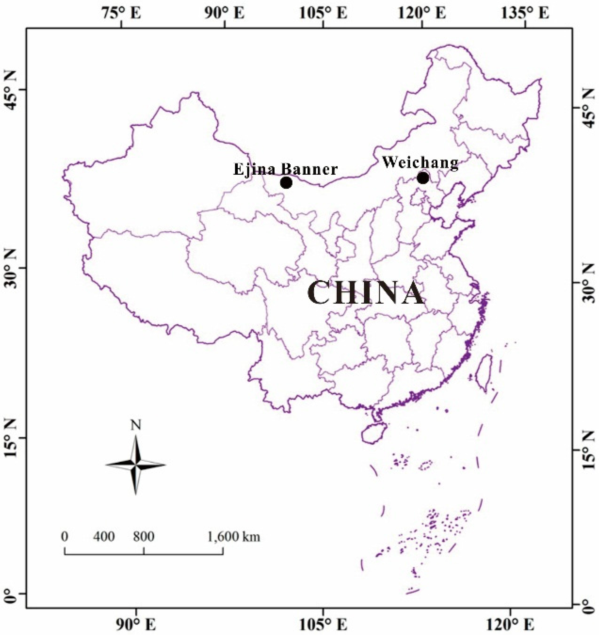
2.1. Study Region

The two study regions were savanna communities situated in Ejina Banner and Weichang county, as shown in Figure 1.

Ejina Banner is one of the most arid regions in China, situated in downstream of the Heihe River Basin (37°45′N–42°40′N, 97°42′E–102°04′E), the second largest inland river basin in China. It is located in the zone of temperate continental and arid climate. The average temperature is 8.3 °C and annual precipitation is approximately 37 mm. Various types of drought tolerant vegetation are randomly distributed across the study region, such as P. euphratica Oliv., Tamarix chinensis Lour., and Astragalus membranaceus Bge. P. euphratica Oliv. is the dominant species of the savanna communities.

Weichang County (41°35′N–42°40′N, 116°32′E–118°14′E) is in the north of Heibei Province, China, at a transition zone between mountainous and highland areas. The climate is transitional between cool temperate continental monsoon plateau and temperate continental monsoon plateau, semi-arid, and semi-humid. The average temperature is 5 °C and annual precipitation is approximately 460 mm. Therefore, steppe and forest steppe are the main vegetation types. B. platyphylla Suk., Pinus sylvestris, and Larix gmelinii are well distributed across the region.

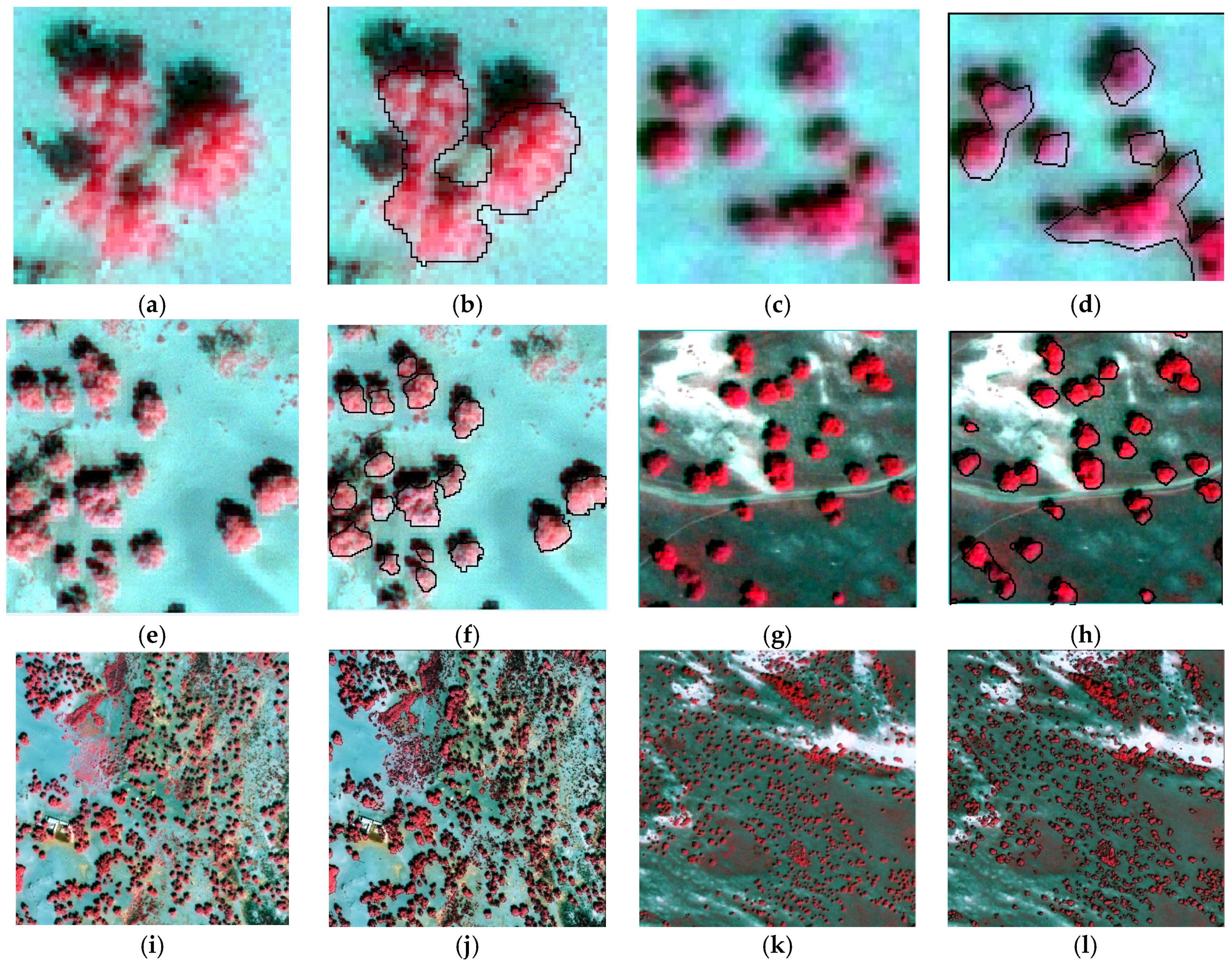
2.2. High Resolution Image Data and Processing

Two high resolution remote sensing images were selected:

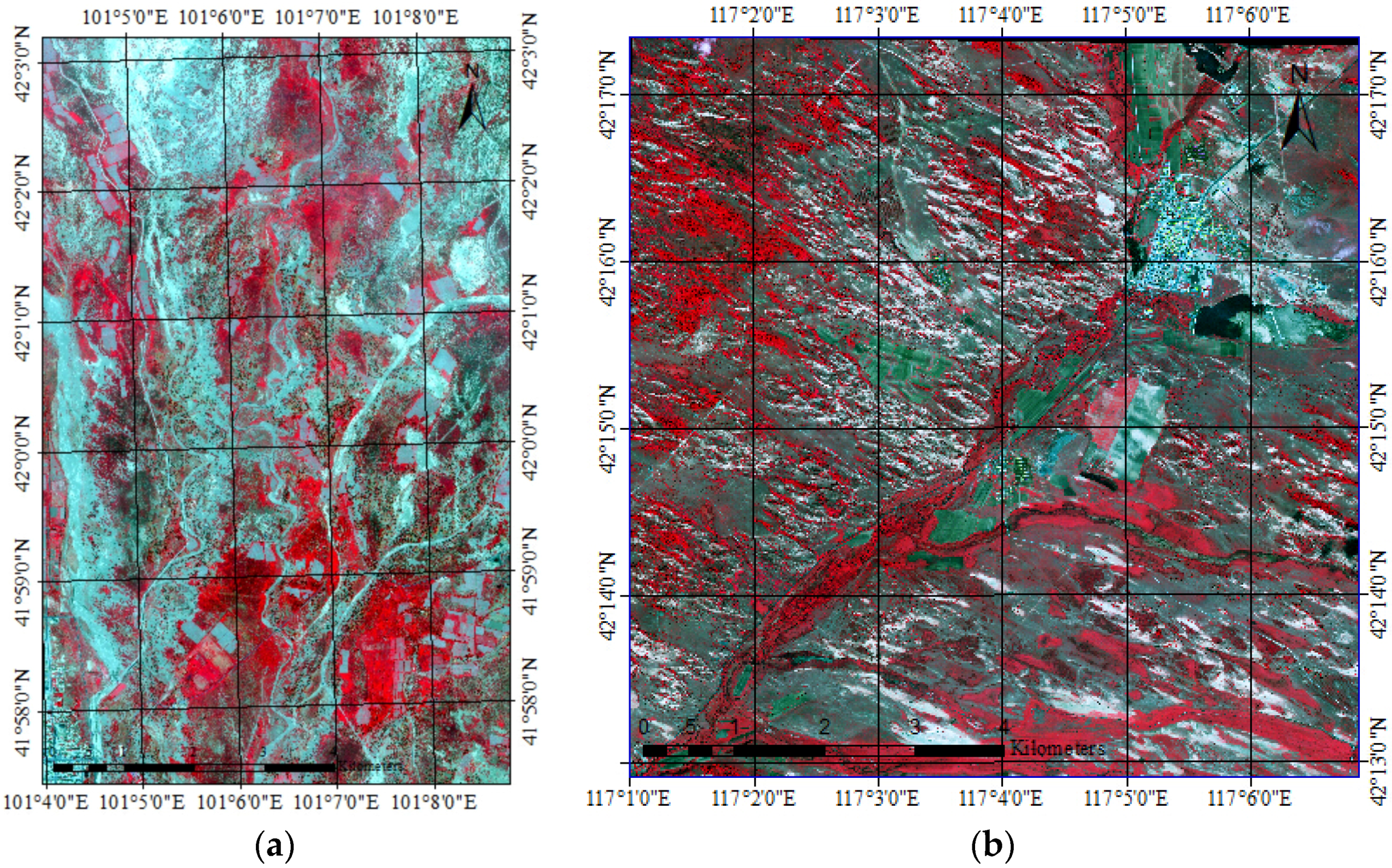
• The Geoeye-1 image acquired at 04:12 a.m. GMT (12:12 p.m. China Time, Beijing), 11 July 2010 (as shown in Figure 2a). Geoeye-1 satellite was launched on 6 September 2008. The satellite provides 0.5 m panchromatic and 2 m multispectral imagery in 15.2 km swaths. Multispectral imagery includes four bands: blue (450–510 nm), green (510–580 nm), red (655–690 nm), and near infra-red (780–920 nm).
• The WorldView-2 image acquired at 06:00 a.m. GMT (14:00 China Time, Beijing), 3 June 2014 (as shown in Figure 2b). The WorldView-2 satellite was launched on 6 October 2009 by Digitalglobe. The satellite provides 1 panchromatic band with spatial resolution of 0.5 m and 8 multispectral bands with spatial resolution of 1.8 m in 16.4 km swaths. The multispectral bands are: coastal (400–450 nm), blue (450–510 nm), green (510–580 nm), yellow (585–625 nm), red (630–690 nm), red edge (705–745 nm), near infra-red 1 (770–895 nm), near infra-red 2 (860–1040 nm).

First, the images were orthorectified using digital elevation model (DEM) data with 1-m resolution to correct for geometric distortions using ENVI 4.8, and a radiometric correction applied. The products were then atmospherically corrected using the FLAASH module included in ENVI 4.8 to retrieve surface reflectance products. Image fusion processing, and combining panchromatic with multispectral bands were performed also using ENVI 4.8. Field observations showed that surface features in study areas included water bodies; farmland; vegetation, such as P. euphratica Oliv., T. chinensis Lour., A. membranaceus Bge., B. platyphylla Suk; etc.

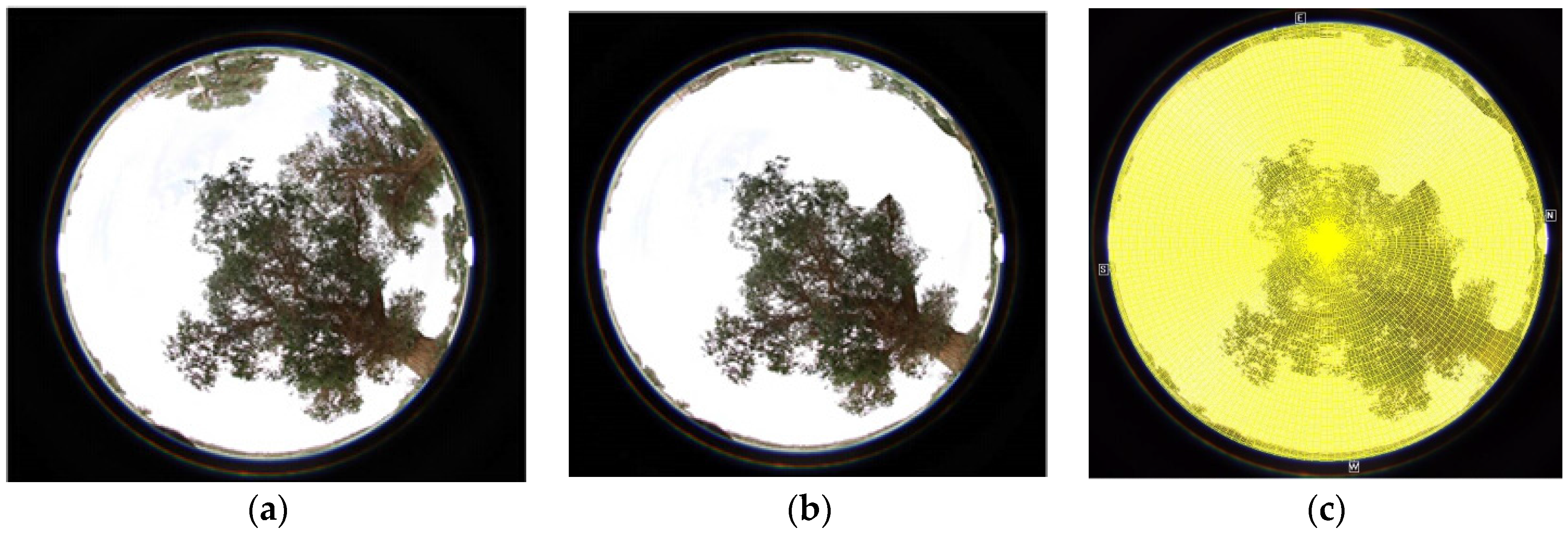
2.3. Sampling Design, Measurements, and Data Processing of Hemispherical Photographs

Field data for Ejina Banner was collected by hemispherical photographs from 2–7 August 2011, in the peak of growing seasons. Field data for Weichang was acquired from 24 July to 2 August 2014. The photographs were all acquired using the same Canon EOS 50D camera with a fish-eye lens, providing orthographic projection and a 180° field of view. The camera was fixed on an automatically leveled Hemiview system (Delta-T Devices Ltd., 130 Low Road, Burwell, Cambridge CB25 0EJ, UK), on a 1.5 m tripod, looking upwards through the canopy. The camera axis was always oriented to magnetic north. All photographs were taken as best possible without direct sunlight. We chose the following settings for the camera: (1) manual mode; (2) fixed fish-eye lens with automatic centrally weighted exposure; (3) manual mode aperture for fixed exposure; (4) high image quality (2272 × 1704 pixels); and (5) JPEG format. Photographs were taken from the sky reference exposure and then corrected with two stops more exposure relative to the open sky conditions [50]. There were approximately 166 hemispherical photographs, including 107 photographs at Ejina Banner and 59 photographs at Weichang county.

Hemispherical photographs were processed using the Hemiview 2.1 software to calculate the CI within canopies. The threshold intensity value was carefully set to obtain binary images that separated sky from the trees [42]. To obtain the gap fraction of a single tree, the original photograph was simplified into separate trees, i.e., one tree in a photo, as shown in Figure 3.

3. Technical Background and Methodology

3.1. LAI and Clumping Index

LAI is defined as half the total green leaf area per unit horizontal ground surface area. Generally, leaves are clumped. Therefore, a CI is introduced to describe the clumping effects. The average transmittance can be expressed as [17]

$$P\left(\theta \right)=\exp \left(\frac{-G\left(\theta \right)\Omega LAI}{\cos \theta }\right)$$

(1)

where $P\left(\theta \right)$ is the gap fraction of the viewing direction within canopies, $\Omega$ is the CI, $G\left(\theta \right)$ is the G function of the viewing direction, $LAI$ represents the true LAI of the vegetation canopy, and $\theta$ is the zenith angle of the viewing direction.

The product of true LAI and CI is the effective LAI, i.e.,

$$LA{I}_{\mathrm{eff}}=\Omega LAI$$

(2)

and the true LAI can be acquired if $LA{I}_{\mathrm{eff}}$ and $\Omega$ are known. The CI = 1 if the spatial distribution of vegetation canopy obeys the Poisson distribution, and the degree of canopy clumping increases with decreasing CI.

Nilson and Kuusk [51] divided forest average gap fractions into two parts: within the tree canopies and between crowns. Clumping effects occur for multiple scales of leaves [52], and so the CI should also be considered at different scales. If leaves and branches are clumped within the single tree, the average transmittance of a single crown can be expressed as

$$P\left(\theta \right)=\exp \left(\frac{-G\left(\theta \right){\Omega }_{1}LAI}{\cos \theta }\right)$$

(3)

where ${\Omega }_1$ is the clumping index within the crown. In this case, the single tree canopy is equivalent to a uniform crown where the leaf area index equals ${\Omega }_{1}LAI$. A second clumping index, ${\Omega }_{\mathrm{t}}$ should be introduced considering both tree crown clustering at ecosystem scale, and clumping within the crown. Therefore, the average transmittance of the whole vegetation canopy can be expressed as

$$P\left(\theta \right)=\exp \left(\frac{-G\left(\theta \right){\Omega }_{\mathrm{t}}LA{I}_{\mathrm{t}}}{\cos \theta }\right)$$

(4)

where $LA{I}_{\mathrm{t}}$ is the average true LAI of the whole vegetation canopy.

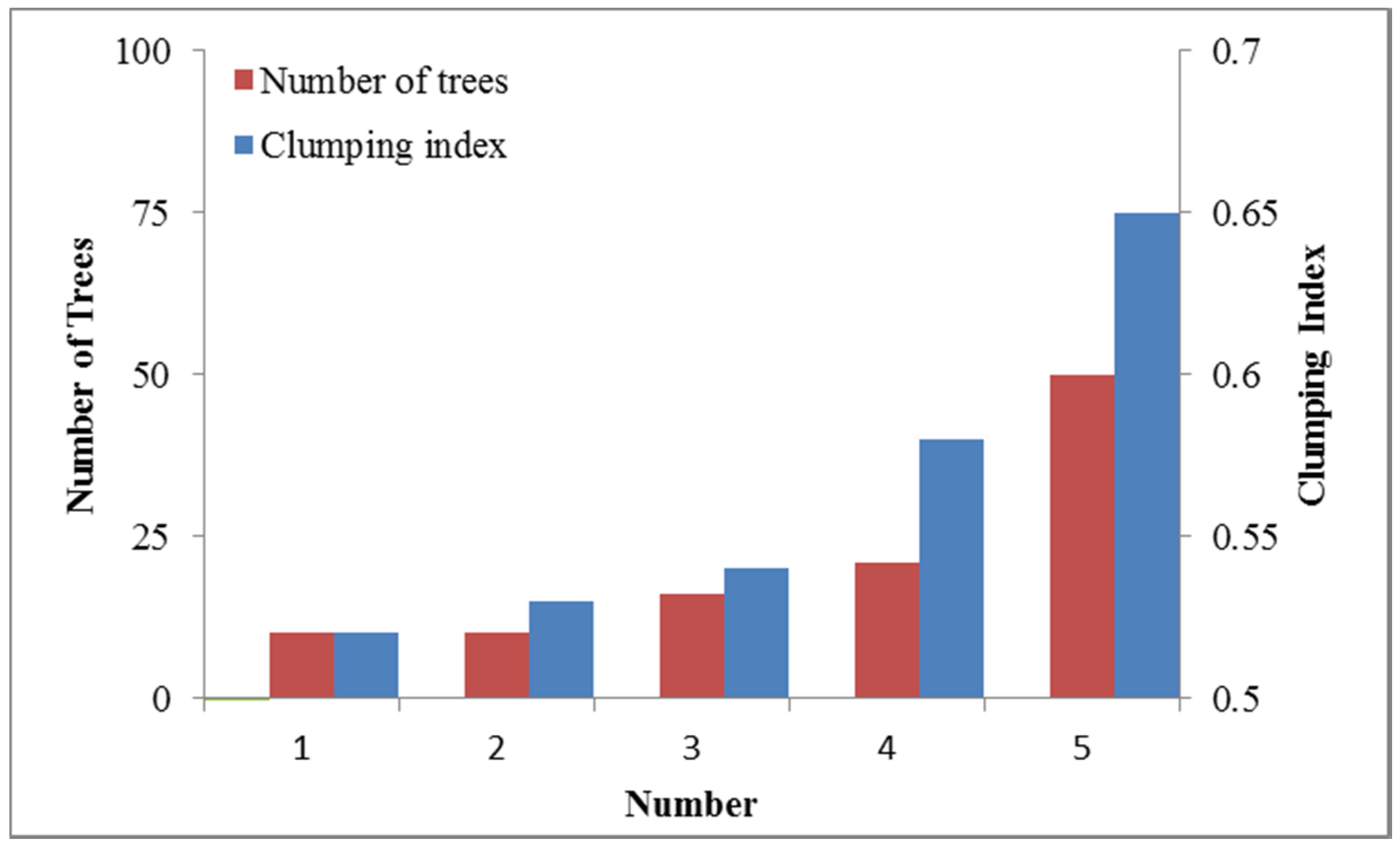
3.2. Single Tree Clumping Index

The gap size distribution derived from the hemispherical photographs can be used to obtain the CI of a single crown. For a canopy with random spatial distribution at any zenith angle, the gap size accumulation function is [18]

$$F\left(\lambda \right)=\left(1+L_p\frac{\lambda }{W_p}\right)exp\left(-L_p\left(1+\frac{\lambda }{W_p}\right)\right)$$

(5)

where $W_p$ is the mean width of the shadow of a leaf projected on a horizontal surface, $L_p$ is the area ratio deriving from a leaf projected on a horizontal surface, and $\lambda$ is the canopy gap size. After modification by Leblanc, CI for any zenith angle can be expressed as [53]

$${\Omega }_1=\frac{1-F_{mr}\left(0\right)}{1-F_m\left(0\right)}\times \frac{\ln \left[F_m\left(0\right)\right]}{\ln \left[F_{mr}\left(0\right)\right]}$$

(6)

where $F_m\left(0\right)$ is the measured accumulated gap fraction larger than zero, i.e., the canopy gap fraction; and $F_{mr}\left(0\right)$ is the gap fraction for the canopy when large gaps are removed for a given $L_p$ and $W_p$.

Given the structure characteristics of P. euphratica Oliv. and B. platyphylla Suk., $L_p$ was first taken as $-\ln \left[F_m\left(0\right)\right]$ to produce the first estimate of $F\left(\lambda \right)$. After some large gaps were removed, a new gap size distribution was computed and $L_p$ was assigned $-\ln \left[F_{mr}\left(0\right)\right]$. Final $L_p$ was found after several iterations until the new distribution, $F_{mr}\left(\lambda \right)$, closely overlaps $F\left(\lambda \right)$.

$W_p$ is influenced by many factors, such as the hemispherical image resolution, foliage distance to the lens, and canopy height. It is set to the most realistic value by iteration [54]. From the finite length averaging method of Lang and Xiang [55], and considering that the plant canopy gaps are generally large, the gap fraction was calculated within finite length = 10 × $L_p$. During processing, photos including a single tree (Figure 3b) were separated into 180 zenith (with 5° interval) and 180 azimuth (with 2° interval) angles, as shown in Figure 3c, and the gap fraction for each grid acquired using Hemiview 2.1 software. The intervals were chosen to distinguish larger gaps (gap fraction = 1 were removed) around tree crown from smaller gaps (gap fractions < 1 were retained) within the canopy. The CI can then be calculated at any zenith angle.

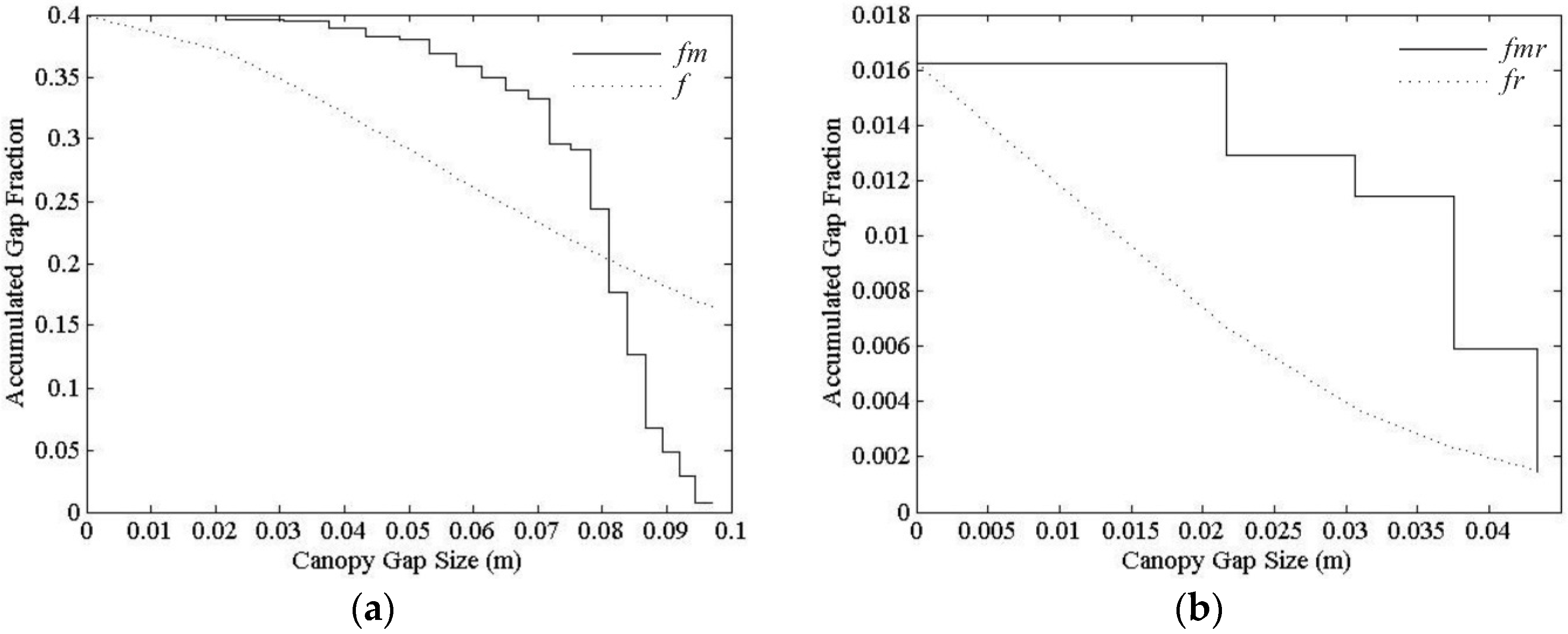
3.3. Clumping Index for Moderate Resolution Pixel

Considering the varied resolution of remote sensing images, clumping effects between crowns are difficult to estimate. Therefore, high resolution images, i.e., the Geoeye-1 and WorldView-2 images, were adopted to estimate the CI within a moderate resolution pixel using average transmittance.

The outline of individual trees must be extracted from the high resolution remote sensing images. Treetop detection was achieved by obtaining the position of each tree using the local maximum with various window sizes [56], decided upon from the average measured crown size. After that, the delineation of the trees was achieved using agent-based region growing algorithms [57]. The relative parameters of trees, including radius, number, and distribution could then be obtained from the high resolution remote sensing images.

For the moderate resolution pixel, the pixel gap fraction is composed of the proportion of larger gaps among tree crowns and smaller gaps within canopies. Considering the clumping effect within each canopy and assuming the background to be bare soil, the transmittance of each part can be described as

$$P\left(\theta \right)=\frac{n\pi R^2\exp \left(\frac{-G\left(\theta \right){\Omega }_{1}LA{I}_{\mathrm{a}1}}{\cos \theta }\right)+\left(A-n\pi R^2\right)}{A}=\exp \left(\frac{-G\left(\theta \right){\Omega }_{\mathrm{t}}LA{I}_{\mathrm{a}2}}{\cos \theta }\right)$$

(7)

where n is the number of crowns, $LA{I}_{\mathrm{a}1}$ and $LA{I}_{\mathrm{a}2}$ are the average true leaf area index of a single tree and the community (i.e., the moderate resolution pixel), respectively; R is the average radius of the crowns; $\theta$ is the sun zenith angle; $G\left(\theta \right)$ is the projection of foliage in the $\theta$ direction; ${\Omega }_1$ and ${\Omega }_{\mathrm{t}}$ are the average CIs of a single tree and of the community (i.e., moderate resolution pixel), respectively; and A is the total area of the moderate resolution pixel. In this paper, $\theta =0^{°}$ and $G\left(\theta \right)$ was derived from leaf angle distribution function, which is related to the leaf distribution within the canopy. Generally, $G\left(\theta \right)$ was assumed to be 0.5.

In savanna growing seasons, the background is full of grass, rather than bare soil. The savanna gap fraction at pixel scale considers several conditions: (1) the gap probability of tree cover, $\exp \left(\frac{-G\left(\theta \right){\Omega }_{1}LA{I}_{\mathrm{a}1}}{\cos \theta }\right)$; (2) the gap probability of grassland, $\exp \left(\frac{-G\left(\theta \right){\Omega }_{\mathrm{g}}LA{I}_{\mathrm{g}}}{\cos \theta }\right)$; and (3) the gap probabilities between tree cover and grassland are assumed to be independent. The total gap fraction can be expressed as,

$$\begin{gathered} P\left(\theta \right)=\frac{n\pi R^2\exp \left(\frac{-G\left(\theta \right){\Omega }_{1}LA{I}_{\mathrm{a}1}}{\cos \theta }\right)\times \exp \left(\frac{-G\left(\theta \right){\Omega }_{\mathrm{g}}LA{I}_{\mathrm{g}}}{\cos \theta }\right)+\left(A-n\pi R^2\right)\times \exp \left(\frac{-G\left(\theta \right){\Omega }_{\mathrm{g}}LA{I}_{\mathrm{g}}}{\cos \theta }\right)}{A} \\ =\exp \left(\frac{-G\left(\theta \right){\Omega }_{\mathrm{t}}LA{I}_{\mathrm{a}2}}{\cos \theta }\right) \end{gathered}$$

(8)

where ${\Omega }_{\mathrm{g}}$ and $LA{I}_{\mathrm{g}}$ are the clumping index and average true leaf area index of grass, respectively.

When grass is in the stage of greened up, the background is composed by grass and bare soil. Then, the transmittance can be expressed as

$$\begin{gathered} P\left(\theta \right)=\frac{n\pi R^2\exp \left(\frac{-G\left(\theta \right){\Omega }_{1}LA{I}_{\mathrm{a}1}}{\cos \theta }\right)+\left(A-n\pi R^2\right)\times F_v\times \exp \left(\frac{-G\left(\theta \right){\Omega }_{\mathrm{g}}LA{I}_{\mathrm{g}}}{\cos \theta }\right)+\left(A-n\pi R^2\right)\times \left(1-F_v\right)}{A} \\ =\exp \left(\frac{-G\left(\theta \right){\Omega }_{\mathrm{t}}LA{I}_{\mathrm{a}2}}{\cos \theta }\right) \end{gathered}$$

(9)

where $F_v$ is the degree of grass coverage.

In the Equations (7) and (8), let

$$\mathrm{m}=\frac{n{R}^2}{A}$$

(10)

where m is the crown density of the pixel. Then within the bare soil background,

$$LA{I}_{\mathrm{a}2}=\pi mLA{I}_{\mathrm{a}1}$$

(11)

and within the floor of grassland,

$$LA{I}_{\mathrm{a}2}=\pi mLA{I}_{\mathrm{a}1}+LA{I}_{\mathrm{g}}$$

(12)

and within the both grass and bare soil background,

$$LA{I}_{\mathrm{a}2}=\pi mLA{I}_{\mathrm{a}1}+\left(1-\pi m\right)F_{v}LA{I}_{\mathrm{g}}$$

(13)

In a pixel with bare soil background, let $C_1=\exp \left(-\frac{G\left(\theta \right)LA{I}_{\mathrm{a}1}}{\cos \theta }\right)$ and $C_2=\exp \left(-\frac{G\left(\theta \right)LA{I}_{\mathrm{a}2}}{\cos \theta }\right)$, whereas for grass floor, let $D_0=\exp \left(-\frac{G\left(\theta \right){\Omega }_{\mathrm{g}}LA{I}_{\mathrm{g}}}{\cos \theta }\right)$, $D_1=\exp \left(-\frac{G\left(\theta \right)LA{I}_{\mathrm{a}1}}{\cos \theta }\right)$, and $D_2=\exp \left(-\frac{G\left(\theta \right)LA{I}_{\mathrm{a}2}}{\cos \theta }\right)$. For the both grass and bare soil background, let $E_0=F_v\left[\exp \left(-\frac{G\left(\theta \right){\Omega }_{\mathrm{g}}LA{I}_{\mathrm{g}}}{\cos \theta }\right)-1\right]+1$, $E_1=\exp \left(-\frac{G\left(\theta \right)LA{I}_{\mathrm{a}1}}{\cos \theta }\right)$, and $E_2=\exp \left(-\frac{G\left(\theta \right)LA{I}_{\mathrm{a}2}}{\cos \theta }\right)$. Then, Equations (7)–(9) can be simplified to, respectively,

$$\frac{{C_2}^{{\Omega }_{\mathrm{t}}}-1}{{C_1}^{{\Omega }_1}-1}=\pi m$$

(14)

$$\frac{{D_2}^{{\Omega }_{\mathrm{t}}}-D_0}{{D_1}^{{\Omega }_1}-1}=\pi m{D}_0$$

(15)

$$\frac{{E_2}^{{\Omega }_{\mathrm{t}}}-E_0}{{E_1}^{{\Omega }_1}-E_0}=\pi m$$

(16)

Once the CI for a single tree (${\Omega }_1$) was calculated, and other parameters, such as average radius of crowns and number of trees, were acquired, the clumping index in the whole pixel (${\Omega }_{\mathrm{t}}$) can be derived.

4. Results

4.1. LAI and Clumping Index of a Single Tree

The clumping index of leaves within the canopy was calculated based on the accumulated gap size distribution using Hemiview software, and the CI can be calculated using Equation (4).

Figure 4 shows the change in $F_m\left(\lambda \right)$ after removing large gaps. The value of f is higher than that of fm for larger gap sizes (Figure 4a). After iteration, most gaps were removed, fr is similar to the new distribution, fmr, and the CI for a single tree can be derived. Twenty-eight hemispherical photos were processed across the two research regions, 14 in Ejina Banner and the balance in Weichang.

Table 1. ${\Omega }_1$ and $LA{I}_{\mathrm{a}1}$ derived from hemispherical photos.

Site	Ejina Banner		Weichang
	${\mathit{\Omega }}_1$	$\mathit{L}\mathit{A}{\mathit{I}}_{\mathbf{a}1}$	${\mathit{\Omega }}_1$	$\mathit{L}\mathit{A}{\mathit{I}}_{\mathbf{a}1}$
Maximum	0.467	4.1	0.668	5.4
Minimum	0.335	3.2	0.344	3.4
Mean	0.393	3.6	0.514	4.8
Variance	0.001	0.073	0.014	0.303

shows the derived ${\Omega }_1$ and $LA{I}_{\mathrm{a}1}$. The average CIs for P. euphratica Oliv. and B. platyphylla Suk. were 0.393 and 0.514, respectively.

4.2. Clumping Index within Moderate Resolution Pixel

After segmentation of images, the radius, distribution, and number of tree crowns can be extracted from high resolution images. Plots with several trees were selected to estimate CIs of P. euphratica Oliv. and B. platyphylla Suk., as shown in Figure 5, and

Table 2. Parameters derived from plots with several trees.

Date	Images	Site	Edge Length (m)	A(${\mathbf{m}}^2$)	n	$\overline{\mathit{R}}\left(\mathbf{m}\right)$	m	${\mathit{\Omega }}_1$	$\mathit{L}\mathit{A}{\mathit{I}}_{\mathbf{a}1}$
11 July 2010	Geoeye-1	Ejina Banner	30	900	3	5.2	0.090	0.393	3.6
			100	10,000	17	5.8	0.057
			500	250,000	633	5.8	0.085
3 June 2014	WorldView-2	Weichang	30	900	10	2.4	0.064	0.514	4.8
			125	15,625	26	4.0	0.027
			500	250,000	834	4.0	0.053

shows the relevant parameters obtained.

Using the parameters listed in Table 2, CI within the moderate resolution pixel can be calculated from Equations (7)–(9). For P. euphratica Oliv., if three trees were distributed in a 30 × 30 m plot, with a bare soil background, as shown in Figure 5b, then CI = 0.304 when $LA{I}_{\mathrm{a}1}=3.6$ and $\overline{R}$ = 5.2 m (i.e., canopy density m = 0.09). The background of B. platyphylla Suk. was also regarded as bare soil. There were 10 trees growing within a 30 × 30 m plot (Figure 5d). The CI for the B. platyphylla Suk. plot was 0.319 when the $LA{I}_{\mathrm{a}1}=4.8$ and $\overline{R}$ = 2.4 m (i.e., crown density m = 0.064). When the plots became larger, the average tree radius changed along with the number of trees, and the CIs are shown in

Table 3. Clumping indices for different plot sizes.

Site	Edge Length of Plots (m)	Clumping Indices of Plots
Ejina Banner	30	0.304
	100	0.306
	500	0.303
Weichang	30	0.319
	125	0.305
	500	0.313

.

5. Discussion

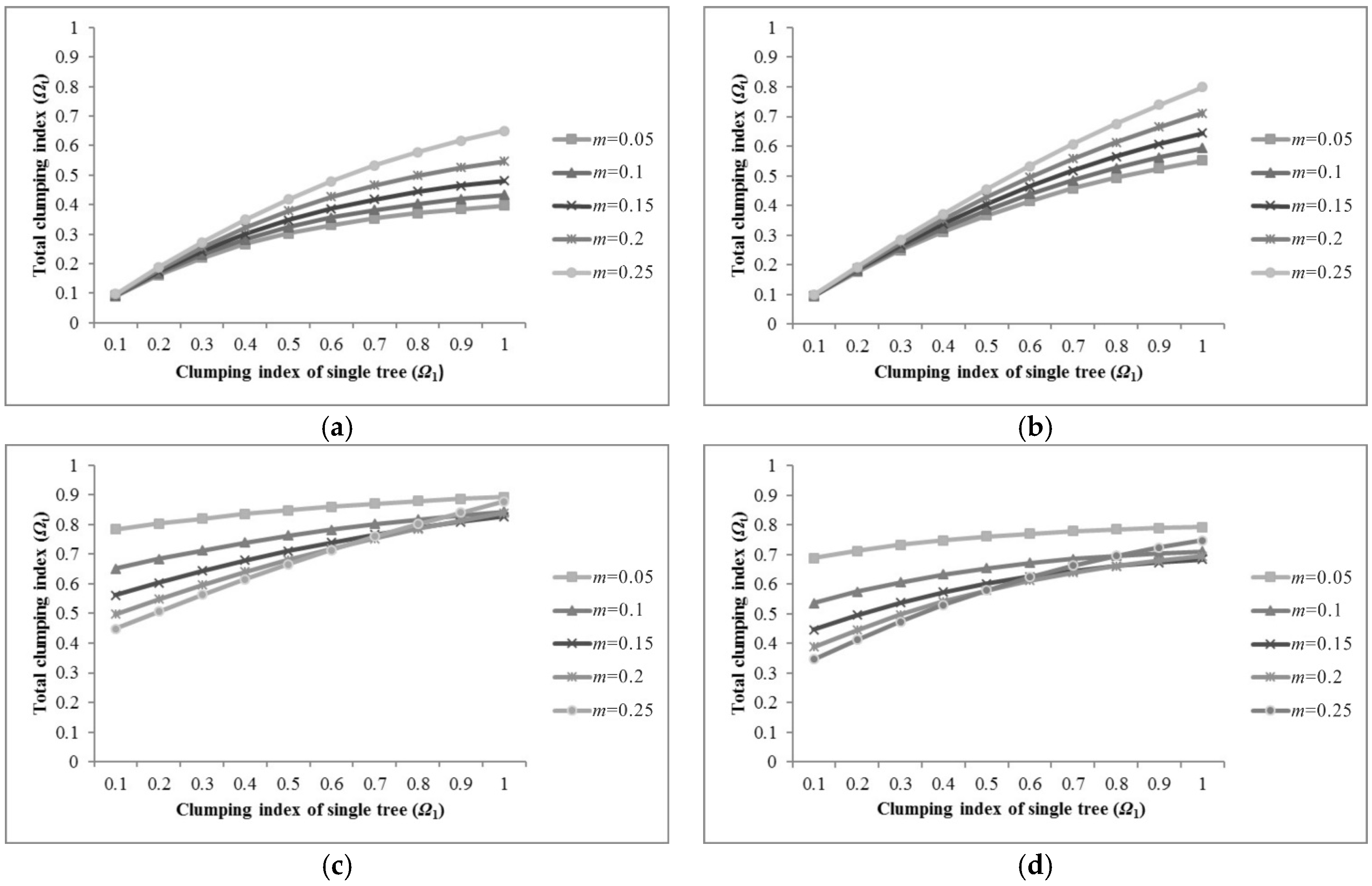
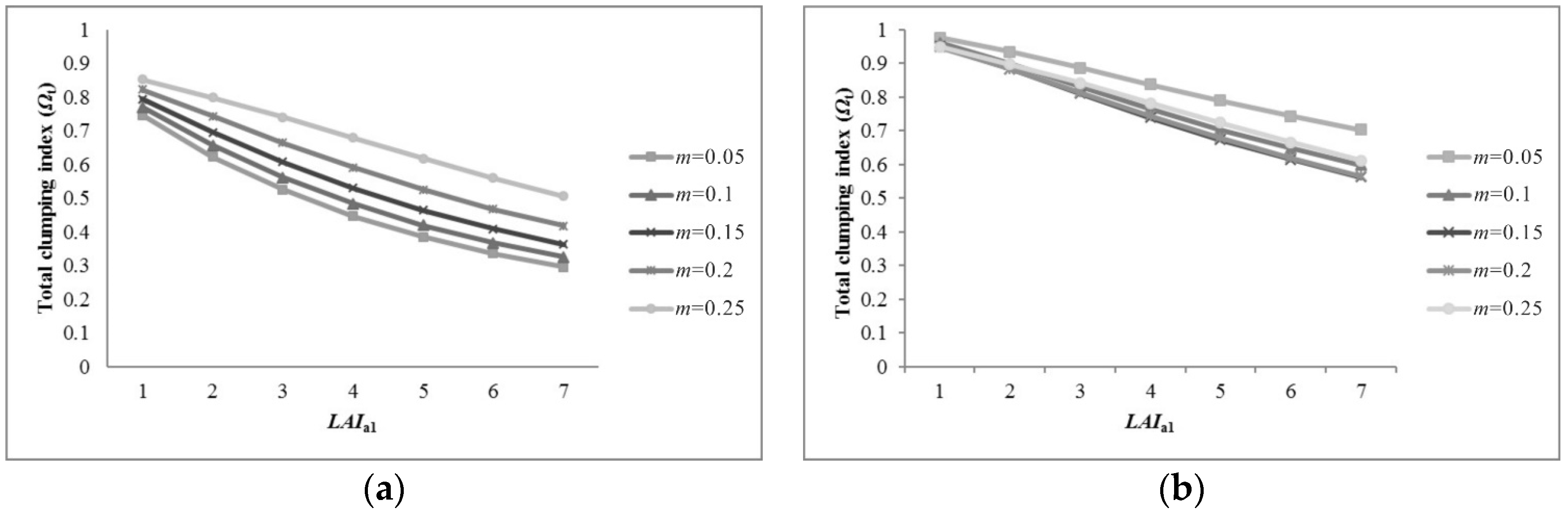
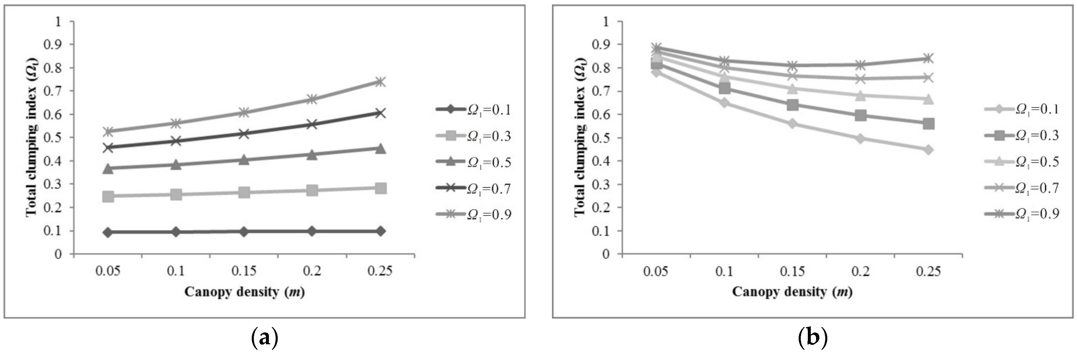
5.1. Sensitivity of Parameters for Pixel Clumping Index Estimation

Figure 6 shows five typical samples in original images, with different numbers of trees and clumping indices (Figure 7). Thus, parameters such as the number of trees, LAI and background all affect the clumping index.

The numerical simulation focused on CI of a pixel. Supposing the moderate pixel size (A) is 100 × 100 m, the trees are randomly distributed within it and have the same height, and their crown shape is spherical. If the radius and number of crowns are R and n, respectively. The single tree leaf area index is $LA{I}_{\mathrm{a}1}$. Then, canopy density, m can be calculated from (9). The pixel CI may be changed by choosing different values of m, n and $LA{I}_{\mathrm{a}1}$. From (9), the maximum m = $\raisebox{1ex}{$1$}\!\left/ \!\raisebox{-1ex}{$\mathsf{\pi }$}\right.$ = 0.3183, and minimum m = 0. Therefore, we set m = 0.05~0.25, with 0.05 intervals. To simplify the problem, grassland CI was assumed = 1 when for the numerical simulation.

Figure 8 shows the relationships between pixel and single tree CI for different LAIs and canopy densities (m). The CI of a single tree can significantly affect pixel CI, and ${\Omega }_{\mathrm{t}}$ increases with increasing ${\Omega }_1$ regardless of the background. When m is small, pixel CI for bare soil was significantly smaller than with grassland. Smaller m implies smaller pixel CI with bare soil background, but the opposite relationship holds for grassland background.

Figure 9 shows that the LAI of a single tree ($LA{I}_{\mathrm{a}1}$) can also affect the pixel CI. The pixel CI decreases with increasing $LA{I}_{\mathrm{a}1}$. There were also significant differences with different backgrounds. In the case of bare soil background, CI for smaller m was always lower for larger m, whereas for grassland background, the opposite trend occurs. From Figure 8 and Figure 9, the growth rate of ${\Omega }_{\mathrm{t}}$ would be slow and maximum of ${\Omega }_{\mathrm{t}}$ decreases with increasing $LA{I}_{\mathrm{a}1}$. As $LA{I}_{\mathrm{a}1}$ increases, the leaves within the canopy become more aggregated, regardless of the background, but the CI for bare soil background decreases more rapidly.

Figure 10 shows that the canopy density can also affect pixel CI. The pixel CI slowly increases with increasing m, regardless of single tree CI for bare soil background, when LAI_a1 = 3, i.e., more trees, the pixel CI was more homogeneous. However, with increasing m, the pixel CI decreased for grassland background, as the increase of trees destroyed the homogeneity of the grassland.

Thus, the background has a significant effect on pixel CI for savannas. The pixel CI is always smaller than the single tree CI for bare soil background, but the opposite is true for grassland background.

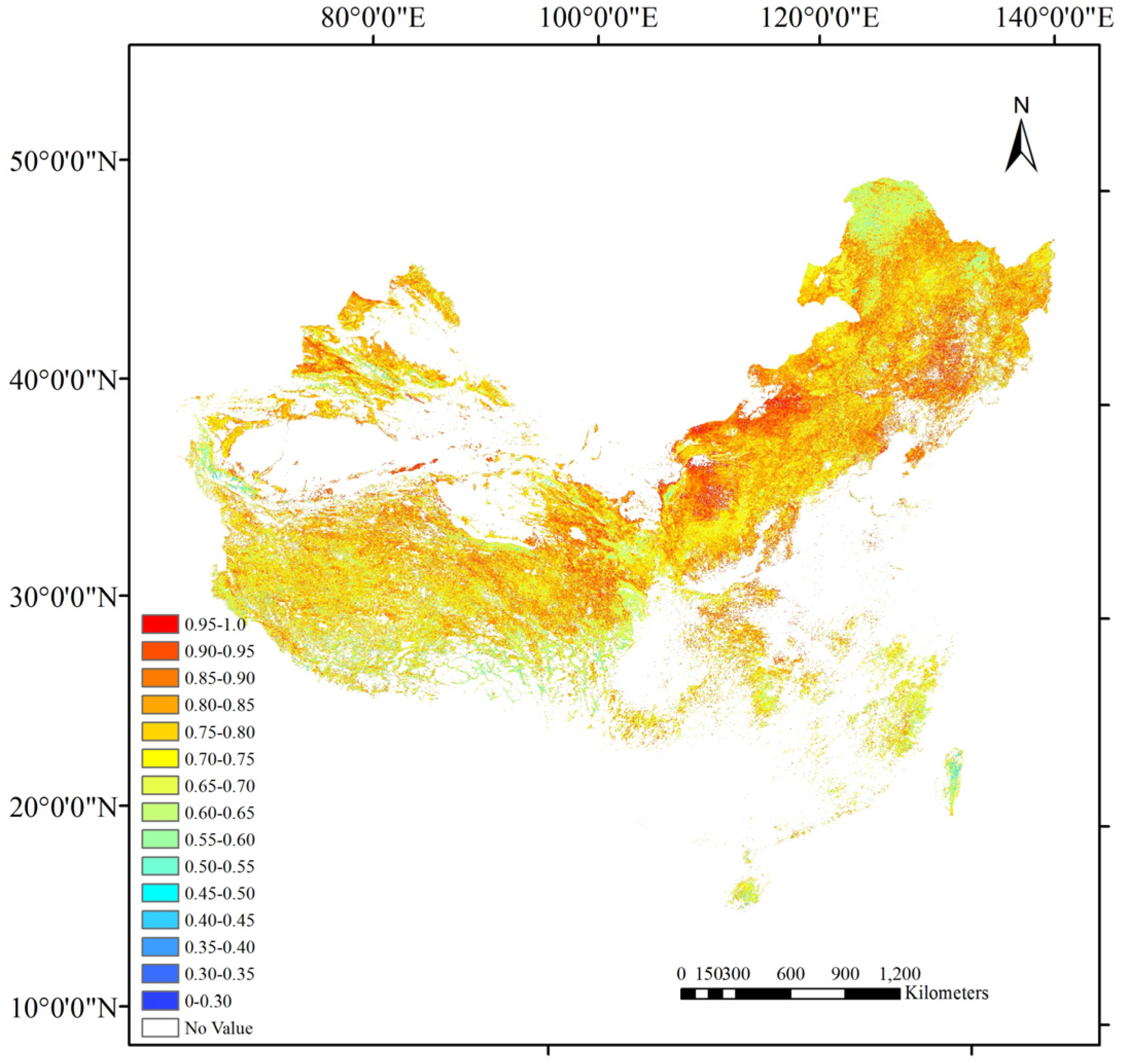
5.2. Comparison with 500 m Clumping Index Products

We also compared the estimated CI with CI products retrieved from MODIS BRDF parameters product by Zhu et al. [32]. The product uses the modified (Ross-Li-H) model to simulate hotspot and darkspot reflectances, to calculate NDHD. The CI products over China’s landmass at 500 m resolution with 8-day intervals were retrieved from 2003 to 2014. Accordingly, monthly CIs were acquired in growing seasons, from June to August, as shown in Figure 11.

Average CIs retrieved by Zhu et al. in growing seasons were 0.73 (June), 0.74 (July) and 0.71 (August) for Ejina Banner, and 0.77 (June), 0.78 (July) and 0.75 (August) for Weichang over 12 years, which show no significant differences.

Plots selected from high resolution remote sensing images must exactly overlap with the clumping index products retrieved by Zhu. The geographic and projected coordinate systems should be the same. Then, CIs of areas where these plots were located could be extracted. The radius and number of tree crowns could also be obtained from the plots, and canopy density (m) calculated. Along with the other relevant parameters, the plot CIs can then be calculated.

We selected plots with 500 m edge length, as shown in Table 2, for the comparisons. CIs retrieved by Zhu et al. were 0.78 (July 2010) for Ejina Banner and 0.80 (June 2014) for Weichang. However, the proposed method with bare soil background produced CI = 0.303 (July 2010) in Ejina Banner (Figure 5i) and 0.313 (June 2014) in Weichang (Figure 5k) from remote sensing image data.

The main reason for this discrepancy is the bare soil backgrounds. The vegetation growing season ranges from April to September across China’s landmass [32], i.e., all types of vegetation, whatever grasslands, croplands, forests, etc., are in the growth stage during these months. The equations for the relationships between CI and NDHD were developed to apply to the whole landmass, and so they do not apply well to the seasonal variation of savannas, which have few trees and no grass in some seasons.

Therefore, we should consider the situation of grassland background, since grass is in the growth stage from the beginning of July to the beginning of September. We used hemispherical photos of grassland for Ejina Banner (August 2010) and Weichang (August 2014), observed downward. We then obtained grassland gap fractions using CAN_EYE software [43] in the range 28%–35% and 22%–30% in Ejina Banner and Weichang, respectively. Measured grassland LAIs ranged from 2.1 to 3.2 in both areas, with average LAIs approximately 2.8. Average grassland CIs were 0.849 and 0.947 in Ejina Banner and Weichang, respectively. Average LAI_a1 = 2.8 for grassland in both areas based on field measurements. Thus, CI = 0.710 for plots in Ejina Banner, and CI = 0.807 in Weichang. Average CIs retrieved by Zhu et al. were 0.74 (August 2010) and 0.75 (August 2014) for these areas, respectively. Thus, the proposed method produces outcomes very close to those retrieved by Zhu et al. [32].

Considering the different backgrounds, the proposed method can effectively estimate pixel clumping index for savannas from a single high resolution remote sensing image for a season, and subsequent ground based measurements.

6. Conclusions

The clumping index of moderate resolution images of savannah regions was calculated using the theory of average transmittance. The clumping index of a single crown was derived from hemispherical photographs using the accumulated gap size distribution. In addition, the radius, distribution, and number of tree crowns were obtained from high resolution images. The proposed method was applied to two study regions in Ejina Banner and Weichang, China, and verified that the method could effectively calculate the clumping index of savannas.

Different factors affecting the clumping index calculation were investigated numerically, single tree clumping index and LAI, canopy density, and backgrounds. Compared with the other 500 m clumping index products over China’s landmass, the proposed method was consistent for the two study regions for grass but not bare soil backgrounds. Thus, savannah seasonal variations should be considered for clumping index retrieval.

However, we isolated single complete trees from hemispherical photos manually, and photo clarity and isolation accuracy will affect the results. Therefore, we should deal with these issues more scientifically in subsequent research. We should also consider other influential factors, such as tree height, canopy shape, etc., to improve the proposed procedure outcomes in further studies, following Chen et al. [8].

This study provides a new concept for subsequent research on savanna conservation and management. Satellite based earth observation techniques as well as ground measurements have a crucial role in monitoring global ecosystems.

References

1. Lacaze, R.; Chen, J.M.; Roujean, J.L.; Leblanc, S.G. Retrieval of vegetation clumping index using hot spot signatures measured by POLDER instrument. Remote Sens. Environ. 2002, 79, 84–95. [Google Scholar] [CrossRef]
2. Anderson, R.C.; Fralish, J.S.; Baskin, J.M. Savannas, Barrens, and Rock Outcrop Plant Communities of North America; Cambridge University Press: Cambridge, UK, 2007. [Google Scholar]
3. McPherson, G.R. Ecology and Management of North American Savannas; University of Arizona Press: Tucson, AZ, USA, 1997. [Google Scholar]
4. Rodríguez-Iturbe, I.; D’Odorico, P.; Porporato, A.; Ridolfi, L. Tree-grass coexistence in Savannas: The role of spatial dynamics and climate fluctuations. Geophys. Res. Lett. 1999, 26, 247–250. [Google Scholar] [CrossRef]
5. Sankaran, M.; Ratnam, J.; Hanan, N.P. Tree-grass coexistence in savannas revisited—Insights from an examination of assumptions and mechanisms invoked in existing models. Ecol. Lett. 2004, 7, 480–490. [Google Scholar] [CrossRef]
6. Baldocchi, D.; Collineau, S. The physical nature of solar radiation in heterogeneous canopies: Spatial and temporal attributes. In Exploitation of Environmental Heterogeneity by Plants: Ecophysiological Processes above-and Belowground; Academic Press: Cambridge, MA, USA, 1994; pp. 21–71. [Google Scholar]
7. Ryu, Y.; Baldocchi, D.D.; Ma, S.; Hehn, T. Interannual variability of evapotranspiration and energy exchange over an annual grassland in California. J. Geophys. Res. Atmos. 2008, 113. [Google Scholar] [CrossRef]
8. Chen, Q.; Baldocchi, D.; Gong, P.; Dawson, T. Modeling radiation and photosynthesis of a heterogeneous savanna woodland landscape with a hierarchy of model complexities. Agric. For. Meteorol. 2008, 148, 1005–1020. [Google Scholar] [CrossRef]
9. Bond, W.J.; Midgley, G.F.; Woodward, F.I.; Hoffman, M.T.; Cowling, R.M. What controls South African vegetation—climate or fire? South Afr. J. Bot. 2003, 69, 79–91. [Google Scholar] [CrossRef]
10. Sankaran, M.; Hanan, N.P.; Scholes, R.J.; Ratnam, J.; Augustine, D.J.; Cade, B.S.; Gignoux, J.; Higgins, S.I.; Le Roux, X.; Ludwig, F.; et al. Determinants of woody cover in African savannas. Nature 2005, 438, 846–849. [Google Scholar] [CrossRef] [PubMed]
11. Yang, X.; Crews, K.A.; Yan, B. Analysis of the pattern of potential woody cover in Texas savanna. Int. J. Appl. Earth Obs. Geoinf. 2016, 52, 527–531. [Google Scholar] [CrossRef]
12. Ramankutty, N.; Foley, J.A. Estimating historical changes in global land cover: Croplands from 1700 to 1992. Glob. Biogeochem. Cycles 1999, 13, 997–1027. [Google Scholar] [CrossRef]
13. Welles, J.M.; Norman, J.M. Instrument for indirect measurement of canopy architecture. Agron. J. 1991, 83, 818–825. [Google Scholar] [CrossRef]
14. Ryu, Y.; Nilson, T.; Kobayashi, H.; Sonnentag, O.; Law, B.E.; Baldocchi, D.D. On the correct estimation of effective leaf area index: Does it reveal information on clumping effects? Agric. For. Meteorol. 2010, 150, 463–472. [Google Scholar] [CrossRef]
15. Chen, J.M.; Menges, C.H.; Leblanc, S.G. Global mapping of foliage clumping index using multi-angular satellite data. Remote Sens. Environ. 2005, 97, 447–457. [Google Scholar] [CrossRef]
16. Chen, J.M.; Liu, J.; Leblanc, S.G.; Lacaze, R.; Roujean, J.L. Multi-angular optical remote sensing for assessing vegetation structure and carbon absorption. Remote Sens. Environ. 2003, 84, 516–525. [Google Scholar] [CrossRef]
17. Nilson, T. A theoretical analysis of the frequency of gaps in plant stands. Agric. Meteorol. 1971, 8, 25–38. [Google Scholar] [CrossRef]
18. Chen, J.M.; Cihlar, J. Plant canopy gap size analysis theory for improving optical measurements of leaf-area index. Appl. Opt. 1995, 34, 6211–6222. [Google Scholar] [CrossRef] [PubMed]
19. Chen, J.M. Optically-based methods for measuring seasonal variation of leaf area index in boreal conifer stands. Agric. For. Meteorol. 1996, 80, 135–163. [Google Scholar] [CrossRef]
20. Norman, J.M.; Jarvis, P.G. Photosynthesis in Sitka spruce (Picea sitchensis (Bong.) Carr.). III. Measurements of canopy structure and interception of radiation. J. Appl. Ecol. 1974, 11, 375–398. [Google Scholar] [CrossRef]
21. Norman, J.M.; Jarvis, P.G. Photosynthesis in Sitka spruce (Picea sitchensis (Bong.) Carr.): V. Radiation penetration theory and a test case. J. Appl. Ecol. 1975, 12, 839–878. [Google Scholar] [CrossRef]
22. Kucharik, C.J.; Norman, J.M.; Murdock, L.; Gower, S.T. Characterizing canopy nonrandomness with a multiband vegetation imager (MVI). J. Geophys. Res. Atmos. 1997, 102, 29455–29473. [Google Scholar] [CrossRef]
23. Nilson, T. Inversion of gap frequency data in forest stands. Agric. For. Meteorol. 1999, 98, 437–448. [Google Scholar] [CrossRef]
24. Privette, J.L.; Tian, Y.; Roberts, G.; Scholes, R.J.; Wang, Y.; Caylor, K.K.; Frost, P.; Mukelabai, M. Vegetation structure characteristics and relationships of Kalahari woodlands and savannas. Glob. Chang. Biol. 2004, 10, 281–291. [Google Scholar] [CrossRef]
25. Chen, J.M.; Black, T.A. Defining leaf area index for non-flat leaves. Plant Cell Environ. 1992, 15, 421–429. [Google Scholar] [CrossRef]
26. Gonsamo, A.; Pellikka, P. The computation of foliage clumping index using hemispherical photography. Agric. For. Meteorol. 2009, 149, 1781–1787. [Google Scholar] [CrossRef]
27. Lemeur, R.; Blad, B.L. A critical review of light models for estimating the shortwave radiation regime of plant canopies. Agric. Meteorol. 1974, 14, 255–286. [Google Scholar] [CrossRef]
28. Jonckheere, I.; Fleck, S.; Nackaerts, K.; Muys, B.; Coppin, P.; Weiss, M.; Baret, F. Review of methods for in situ leaf area index determination: Part I. Theories, sensors and hemispherical photography. Agric. For. Meteorol. 2004, 121, 19–35. [Google Scholar] [CrossRef]
29. Pisek, J.; Chen, J.M.; Lacaze, R.; Sonnentag, O.; Alikas, K. Expanding global mapping of the foliage clumping index with multi-angular POLDER three measurements: Evaluation and topographic compensation. ISPRS J. Photogramm. Remote Sens. 2010, 65, 341–346. [Google Scholar] [CrossRef]
30. Hill, M.J.; Román, M.O.; Schaaf, C.B.; Hutley, L.; Brannstrom, C.; Etter, A.; Hanan, N.P. Characterizing vegetation cover in global savannas with an annual foliage clumping index derived from the MODIS BRDF product. Remote Sens. Environ. 2011, 115, 2008–2024. [Google Scholar] [CrossRef]
31. Pisek, J.; Govind, A.; Arndt, S.K.; Hocking, D.; Wardlaw, T.J.; Fang, H.; Matteucci, G.; Longdoz, B. Intercomparison of clumping index estimates from POLDER, MODIS, and MISR satellite data over reference sites. ISPRS J. Photogramm. Remote Sens. 2015, 101, 47–56. [Google Scholar] [CrossRef]
32. Zhu, G.; Ju, W.; Chen, J.M.; Gong, P.; Xing, B.; Zhu, J. Foliage clumping index over China’s landmass retrieved from the MODIS BRDF parameters product. IEEE Trans. Geosci. Remote Sens. 2012, 50, 2122–2137. [Google Scholar] [CrossRef]
33. He, L.; Chen, J.M.; Pisek, J.; Schaaf, C.B.; Strahler, A.H. Global clumping index map derived from the MODIS BRDF product. Remote Sens. Environ. 2012, 119, 118–130. [Google Scholar] [CrossRef]
34. He, L.; Liu, J.; Chen, J.M.; Croft, H.; Wang, R.; Sprintsin, M.; Zheng, T.; Ryu, Y.; Pisek, J.; Gonsamo, A.; et al. Inter-and intra-annual variations of clumping index derived from the MODIS BRDF product. Int. J. Appl. Earth Obs. Geoinf. 2016, 44, 53–60. [Google Scholar] [CrossRef]
35. Canisius, F.; Chen, J.M. Retrieving forest background reflectance in a boreal region from Multi-angle Imaging SpectroRadiometer (MISR) data. Remote Sens. Environ. 2007, 107, 312–321. [Google Scholar] [CrossRef]
36. Pisek, J.; Chen, J.M.; Miller, J.R.; Freemantle, J.R.; Peltoniemi, J.I.; Simic, A. Mapping forest background reflectance in a boreal region using multiangle compact airborne spectrographic imager data. IEEE Trans. Geosci. Remote Sens. 2010, 48, 499–510. [Google Scholar] [CrossRef]
37. Gonsamo, A.; Chen, J.M. Improved LAI algorithm implementation to MODIS data by incorporating background, topography, and foliage clumping information. IEEE Trans. Geosci. Remote Sens. 2014, 52, 1076–1088. [Google Scholar] [CrossRef]
38. Olofsson, P.; Eklundh, L. Estimation of absorbed PAR across Scandinavia from satellite measurements. Part II: Modeling and evaluating the fractional absorption. Remote Sens. Environ. 2007, 110, 240–251. [Google Scholar] [CrossRef]
39. Chen, J.M.; Pavlic, G.; Brown, L.; Cihlar, J.; Leblanc, S.G.; White, H.P.; Hall, R.J.; Peddle, D.R.; King, D.J.; Trofymow, J.A.; et al. Derivation and validation of Canada-wide coarse-resolution leaf area index maps using high-resolution satellite imagery and ground measurements. Remote Sens. Environ. 2002, 80, 165–184. [Google Scholar] [CrossRef]
40. Chianucci, F.; Macfarlane, C.; Pisek, J.; Cutini, A.; Casa, R. Estimation of foliage clumping from the LAI-2000 plant canopy analyzer: Effect of view caps. Trees 2015, 29, 355–366. [Google Scholar] [CrossRef]
41. Van Gardingen, P.R.; Jackson, G.E.; Hernandez-Daumas, S.; Russell, G.; Sharp, L. Leaf area index estimates obtained for clumped canopies using hemispherical photography. Agric. For. Meteorol. 1999, 94, 243–257. [Google Scholar] [CrossRef]
42. Walter, J.M.N.; Fournier, R.A.; Soudani, K.; Meyer, E. Integrating clumping effects in forest canopy structure: An assessment through hemispherical photographs. Can. J. Remote Sens. 2003, 29, 388–410. [Google Scholar] [CrossRef]
43. Demarez, V.; Duthoit, S.; Baret, F.; Weiss, M.; Dedieu, G. Estimation of leaf area and clumping indexes of crops with hemispherical photographs. Agric. For. Meteorol. 2008, 148, 644–655. [Google Scholar] [CrossRef] [Green Version]
44. Chianucci, F.; Cutini, A. Estimation of canopy properties in deciduous forests with digital hemispherical and cover photography. Agric. For. Meteorol. 2013, 168, 130–139. [Google Scholar] [CrossRef]
45. Pekin, B.; Macfarlane, C. Measurement of crown cover and leaf area index using digital cover photography and its application to remote sensing. Remote Sens. 2009, 1, 1298–1320. [Google Scholar] [CrossRef]
46. Kucharik, C.J.; Norman, J.M.; Gower, S.T. Characterization of radiation regimes in nonrandom forest canopies: Theory, measurements, and a simplified modeling approach. Tree Physiol. 1999, 19, 695–706. [Google Scholar] [CrossRef] [PubMed]
47. Zhao, F.; Strahler, A.H.; Schaaf, C.L.; Yao, T.; Yang, X.; Wang, Z.; Schull, M.A.; Román, M.O.; Woodcock, C.E.; Olofsson, P.; et al. Measuring gap fraction, element clumping index and LAI in Sierra Forest stands using a full-waveform ground-based lidar. Remote Sens. Environ. 2012, 125, 73–79. [Google Scholar] [CrossRef]
48. Hoffmann, W.A.; da Silva, E.R., Jr.; Machado, G.C.; Bucci, S.J.; Scholz, F.G.; Goldstein, G.; Meinzer, F.C. Seasonal leaf dynamics across a tree density gradient in a Brazilian savanna. Oecologia 2005, 145, 306–315. [Google Scholar] [CrossRef] [PubMed]
49. Scholes, R.J.; Frost, P.G.; Tian, Y. Canopy structure in savannas along a moisture gradient on Kalahari sands. Glob. Chang. Biol. 2004, 10, 292–302. [Google Scholar] [CrossRef]
50. Zhang, Y.; Chen, J.M.; Miller, J.R. Determining digital hemispherical photograph exposure for leaf area index estimation. Agric. For. Meteorol. 2005, 133, 166–181. [Google Scholar] [CrossRef]
51. Nilson, T.; Kuusk, A. Improved algorithm for estimating canopy indices from gap fraction data in forest canopies. Agric. For. Meteorol. 2004, 124, 157–169. [Google Scholar] [CrossRef]
52. Chen, J.M.; Leblanc, S.G. A four-scale bidirectional reflectance model based on canopy architecture. IEEE Trans. Geosci. Remote Sens. 1997, 35, 1316–1337. [Google Scholar] [CrossRef]
53. Leblanc, S.G. Correction to the plant canopy gap size analysis theory used by the tracing radiation and architecture of canopies instrument. Appl. Opt. 2002, 41, 7667–7670. [Google Scholar] [CrossRef] [PubMed]
54. Leblanc, S.G.; Chen, J.M.; Fernandes, R.; Deering, D.W.; Conley, A. Methodology comparison for canopy structure parameters extraction from digital hemispherical photography in boreal forests. Agric. For. Meteorol. 2005, 129, 187–207. [Google Scholar] [CrossRef]
55. Lang, A.R.G.; Xiang, Y. Estimation of leaf area index from transmission of direct sunlight in discontinuous canopies. Agric. For. Meteorol. 1986, 37, 229–243. [Google Scholar] [CrossRef]
56. Zhen, Z.; Quackenbush, L.J.; Zhang, L. Impact of tree-oriented growth order in marker-controlled region growing for individual tree crown delineation using airborne laser scanner (ALS) data. Remote Sens. 2014, 6, 555–579. [Google Scholar] [CrossRef]
57. Zhen, Z.; Quackenbush, L.J.; Stehman, S.V.; Zhang, L. Agent-based region growing for individual tree crown delineation from airborne laser scanning (ALS) data. Int. J. Remote Sens. 2015, 36, 1965–1993. [Google Scholar] [CrossRef]
Figure 1. Study region locations.
Remotesensing 09 00052 g001
Figure 2. False color images of the study regions: (a) Geoeye-1 image, Ejina Banner, downstream of the Heihe River Basin, Inner Mongolia, China; (b) WorldView-2 image, Weichang county, Hebei Province, China. (False color composite: Red-Near infrared (for Geoeye-1 images)/Red-Near infrared 1 (for WorldView-2 images), Red and Green).
Remotesensing 09 00052 g002
Figure 3. Typical hemispherical photograph from the experiment sites: (a) original; (b) modified to include only a single tree; (c) divided by sky map using Hemiview 2.1 software.
Remotesensing 09 00052 g003
Figure 4. Gap size distribution (a) before and (b) after large gaps removal.
Remotesensing 09 00052 g004
Figure 5. (al) Image segmentation and crown extraction with different edge lengths in false color. (a,b,e,f,i,j) Geoeye-1 image, plots of P. euphratica Oliv, located in Ejina Banner, Inner Mongolia, China. (c,d,g,h,k,l) WorldView-2 image, plots of B. platyphylla Suk., located in Weichang, Heibei Province, China. Plots with edge length (ad) 30 m; (e,f) 100 m; (g,h) 125 m; (il) 500 m. (a,c,e,g,i,k) original multispectral images of the selected plots; (b,d,f,h,j,l) segmented tree crowns.
Remotesensing 09 00052 g005
Figure 6. Typical original multispectral images.
Remotesensing 09 00052 g006
Figure 7. Number of trees and clumping index for each plot from the images in Figure 6.
Remotesensing 09 00052 g007
Figure 8. Pixel and single tree clumping index for different LAIs and canopy densities (m). (a,b) bare soil background; (c,d) grassland background. The clumping index and average true LAI of grass were assumed = 1 and 1.5, respectively; (a,c) average true LAI of a single tree = 3; (b,d) average true LAI of a single tree = 5.
Remotesensing 09 00052 g008
Figure 9. Pixel clumping index and L A I a 1 for different canopy densities (m) when Ω 1 = 0.9 : (a) bare soil background; (b) grassland background. The clumping index and average true LAI of grass were assumed = 1 and 1.5, respectively.
Remotesensing 09 00052 g009
Figure 10. Pixel clumping index and canopy density for different single tree clumping indices when LAIa1 = 3. (a) Bare soil background; (b) Grassland background. The clumping index and average true LAI of grass were assumed = 1 and 1.5, respectively.
Remotesensing 09 00052 g010
Figure 11. Clumping index products over China’s landmass at 500 m resolution (July 2010) retrieved by Zhu et al. [32].
Remotesensing 09 00052 g011