UAV-Borne Profiling Radar for Forest Research

Abstract

Microwave Radar is an attractive solution for forest mapping and inventories because microwave signals penetrates into the forest canopy and the backscattering signal can provide information regarding the whole forest structure. Satellite-borne and airborne imaging radars have been used in forest resources mapping for many decades. However, their accuracy with respect to the main forest inventory attributes substantially varies depending on the wavelength and techniques used in the estimation. Systems providing canopy backscatter as a function of canopy height are, practically speaking, missing. Therefore, there is a need for a radar system that would enable the scientific community to better understand the radar backscatter response from the forest canopy. Consequently, we undertook a research study to develop an unmanned aerial vehicle (UAV)-borne profiling (i.e., waveform) radar that could be used to improve the understanding of the radar backscatter response for forestry mapping and inventories. A frequency modulation continuous waveform (FMCW) profiling radar, termed FGI-Tomoradar, was introduced, designed and tested. One goal is the total weight of the whole system is less than 7 kg, including the radar system and georeferencing system, with centimetre-level positioning accuracy. Achieving this weight goal would enable the FGI-Tomoradar system to be installed on the Mini-UAV platform. The prototype system had all four linear polarization measuring capabilities, with bistatic configuration in Ku-band. In system performance tests in this study, FGI-Tomoradar was mounted on a manned helicopter together with a Riegl VQ-480-U laser scanner and tested in several flight campaigns performed at the Evo site, Finland. Airborne laser scanning data was simultaneously collected to investigate the differences and similarities of the outputs for the same target area for better understanding the penetration of the microwave signal into the forest canopy. Preliminary analysis confirmed that the profiling radar measures a clear signal from the canopy structure and has substantial potential to improve our understanding of radar forest mapping using the UAV platform.

1. Introduction

Radar is an active sensor that transmits radio or microwave radiation and record echoes from the target area. Imaging radars use microwaves with wavelengths that range from centimetres to metres. In the case of forestry, it is well known that the transmitted radar radiation penetrates into the forest canopy and that the penetration and interaction of the radiation strongly depend on the system parameters (e.g., wavelength, polarization) and the target features (e.g., moisture, forest structures, biomass). Therefore, microwave radar is an attractive system for forest mapping and forest resources estimating. Satellite-borne and airborne imaging radars, primarily synthetic aperture radars (SAR), have been studied and used in forest mapping for many decades [1,2,3,4,5]. Due to its all-weather imaging capability, satellite SAR enables wide-area mapping, which might not be possible to utilize other remote sensing techniques. The primary technique used in forest mapping is based on SAR intensity information. The SAR intensity is the strength of the backscattered signal comparing to the transmitted signal, and it depends not only on the system wavelength and the polarization but also on the target parameters. The target parameters, such as forest biomass, canopy density and tree type, must be taken into account and calibrated in advance because from a physics viewpoint the propagation of a radio frequency (RF) signal is influenced by the objects or the materials through which it passes. The characteristics of different radar wavelengths (i.e., microwave bands) with respect to the use of forest biomass from SAR data are discussed in Le Toan et al. [6]. According to Le Toan et al. [6], the SAR backscattering intensity of longer wavelengths (e.g., the L and P bands, which have wavelengths of about 20 and 60 cm, respectively) is more effective than that of shorter microwaves (e.g., the X and C bands, which have wavelengths of 2–6 cm) in forest biomass estimation. Using short microwaves, the scattering mainly occurs at the top parts of the forest canopy, whereas in long microwaves the signal is more dependent on the forest tree trunks. Thus, the tree trunk and the forest stem volume can be better mapped with a longer wavelength microwave signal. Recently, SAR satellite systems with short wavelengths (i.e., the X band) have also been found powerful in forest resources mapping when using forest canopy height measurements rather than SAR intensity information. When X-band SAR elevation measurements obtained by using SAR stereo-radargrammetry [7,8] or SAR interferometry [9,10] are subtracted from the terrain elevation values known from other source, forest tree height can be estimated, and consequently, forest stem volume and biomass can be estimated. In X-band SAR satellite data, the backscattering signal per resolution cell is coherently averaged, and the phase centre of the echo is relatively close to the top of the forest canopy. Therefore, the elevation measurement is highly correlated with the tree height. A drawback is that the terrain elevation cannot be easily observed from the measurements. Therefore, a digital terrain model obtained from another source, typically airborne laser scanning (ALS), is required to assist in obtaining tree height estimates.

However, it has also been shown that a short microwave radar signal penetrates deeply into the forest canopy, even to the ground level. Stand profiles that present tree height and density in forest using helicopter-borne C-band (5.4 GHz) microwave radar were first reported by Bernard et al. [11]. Subsequent studies on forest inventory using microwave radar data have been conducted in the past decades [12,13,14,15,16]. A helicopter-borne profiling radar system known as HUTSCAT was designed and demonstrated by Hallikainen et al. [14]. Subsequently, intensive studies were performed based on HUTSCAT measurement. Based on these results, the nadir-looking profiling radar response from boreal forest clearly not only contains a signal from the ground surface but also echoes above-ground tree structures, which implies that gathering tree height estimation together with canopy density information can be achieved using a single instrument. In practice, these systems are similar to waveform LiDARs, which have been used in laser scanning since the early 2000s, and obtain similar data. In the early 2000s, the primary challenge was to accurately determine the location of the radar antenna and its orientation. Therefore, the problem of accurately locating the target remained unidentified. When airborne LiDARs emerged, the development of profiling radar did not continue. However, a number of studies have focused on unmanned air vehicle (UAV)-based radar systems, such as Xing et al. [17] and WeiB et al. [18], in which the investigated radar technology was SAR rather than FMCW profile radar. A 3D imaging version of radar, as proposed, e.g., by Elachi [19], was not realized in operative airborne remote sensing since airborne laser scanning turned out to be a more cost-effective technique for forest inventory. However, profiling radar was compared with other remote sensing techniques for forestry with respect to information content by Hyyppä et al. [20]. Laser scanning was previously found to be superior to forest inventory by Hyyppä et al. [21].

Since the 1990s, direct positioning and orientation technology has substantially improved. However, in the scientific community, a need remains to better understand the radar response from forest structures. Therefore, there is a demand for a profiling radar system equipped with state-of-the-art positioning technology, which would assist scientists to more comprehensively understand the radar and SAR response from forest and possibly develop more accurate methods of satellite SAR-based forest resource mapping. The goals of this study were to design, construct, and test a light-weight short wavelength profiling radar system capable of acquiring highly accurate vertical intensity profiles from forest using both a helicopter and a UAV platform, as well as to compare these vertical intensity profiles with other remote sensing data from the same test sites.

In general, we tested the prototype profile radar at the EVO test site in this research [22]. ALS data was collected from the same area on the following day. More accurate information on the vertical structure of forests (i.e., a canopy cross section, attenuation, canopy gaps) can be achieved by combining ALS and radar profile data. Such an approach enables the calculation of the direct reflection from the ground due to canopy gaps and volumetric scattering from the canopy due to the penetration. More explicitly, In this research, (1) we investigated whether UAV-borne FMCW profile radar is feasible with latest developed components and state-of-the-art devices; (2) we carried out the range calibration based on ground test to testify the system range linearity; (3) we confirmed the profile radar can penetrate boreal forest from tree canopy top to ground level through branches and trunks, and extracted the ground and vertical structure information; (4) we assured that, by combining topography information collected by laser scanner and density information unveiled by profile information archived by Tomoradar, a more composite forest model can be generated to assist the understanding of how RF signal propagates in boreal forest.

2. FGI-Tomoradar Development

UAV/small plane based bistatic antenna profile radar termed Tomoradar was constructed at FGI. A pencil-beam FM-CW scatterometer provided the backscattering properties of a target as a function of range. A two-antenna configuration in the Ku-band provided higher sensitivity for all polarization modes compared to a single antenna solution. Both backscattered amplitudes from horizontal and vertical polarization channel were recorded to provide a polarimetric waveform radar image. The advantages of Tomoradar over the HUTSCAT system are shown in

Table 1. Technical Specification Comparison between Tomoradar and HUSCAT.

	Tomoradar	HUSCAT
Modulation frequency fmod	163 Hz	60 Hz
Distance range	10–300 m	8–167 m
Range resolution	15 cm	65 cm
Centre frequency	14 GHz (2.1 cm)	9.8 GHz (3.1 cm)
		5.4 GHz (5.6 cm)
Spatial resolution	two-way antenna beamwidth <6°	3.8° (9.8 GHz)
		4.7° (5.4 GHz)
Polarization	Full	Full
A/D converter	12 bits	12 bits
Recoded Data	IF amplifier data	FFT results only
FFT	Software-based	Hardware-based
Georeference Accuracy	1 cm + 1 ppm	Unspecified
Power Consumption	20 W	several hundred watts based on the configurations
Weight	Less than 5 kg	approximately 50–100 kg, including antenna support
Data rate	2.5 M/S	80 KB/S

.

It can be observed that except for lower spatial resolution, Tomoradar easily outperforms HUTSCAT. In addition to the higher range resolution and modulation frequency and lower weight and power consumption, the fast Fourier transform (FFT) calculation can be performed by the software in real time in Tomoradar. Thus, after the down-conversion of the received RF echo to an intermediate frequency (IF) signal, high-pass filtering and IF amplification, the raw IF signal can be sampled at a high sampling rate by a digitizer, which is synchronized to the original triangular waveform used to modulate the microwave oscillator.

The system weight and power consumption of Tomoradar are significantly lower than HUTSCAT as Table 1 presents, which enables Tomoradar’s use on a UAV platform. The UAV platform offers following advantages comparing with other airborne platforms:

• UAV platform is more cost-effective than helicopter or fixed-wing platforms, and the field test cost is considerable lower than for other manned aircrafts.
• There are fewer regulatory restrictions on the UAV platform, such as test permission applications. In Finland, the lightweight Mini-UAV platform is allowed to perform field tests less than 200 m in operation altitude without special permission in unrestricted areas with line of sight operation condition. In addition, UAV-borne Tomoradar offers enhanced flexibility in empirical tests of theoretical research.
• The UAV platform is particularly suitable for the spatial resolution of Tomoradar. Single-tree-level forestry investigation requires much lower operation altitude—tens meters, based on current spatial resolution (6 degrees).
• Finally, because the current Tomoradar is not equipped with a mechanical scanning supporter, it can only collect the profile data along the trajectory rather than a scanning imaging radar. The operational efficiency using the helicopter platform is low: only the backscatter reflected by the targets at nadir direction with a few meters swath width can be collected. To investigate a normal plot (i.e., 32 × 32 m²), assuming the flight height is 50 m; at least 7 parallel scans are required with current antenna configuration, which involves extra effort for the helicopter pilot. Meanwhile, the flight route can be defined with most flying control programs for the UAV platform. Moreover, the scanning supporter might cause a polarization-change problem.

Tomoradar is also equipped with a high-accuracy georeferencing system, which consists of a high-quality global navigation satellite system (GNSS) receiver and a tactical-grade inertial measurement unit (IMU). The georeferencing system measures the helicopter flight trajectory with centimetre-level accuracy, which avoids the problems that HUTSCAT faced.

Tomoradar was designed for forest inventory. Thus, the three main requirements for FGI-Tomoradar were as follows: (1) accurate measurement of the backscattering coefficient with good range resolution; (2) multiple polarization capability for comparing measurements from different polarizations; and (3) simultaneously operable multiple polarization, light weight and low power consumption for UAV-based forest inventory tasks.

2.1. System Design

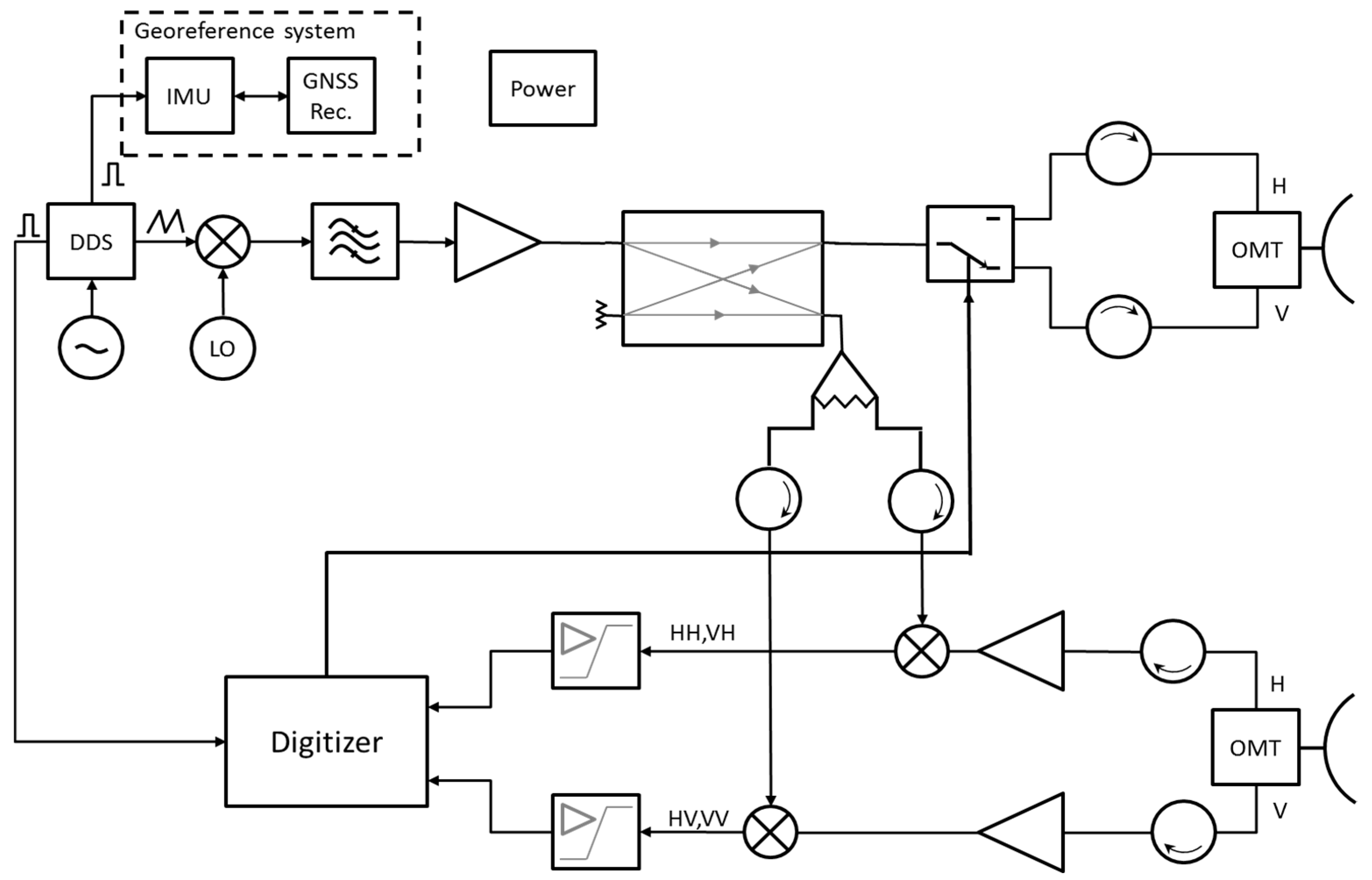
A simplified block diagram of Tomoradar is presented in Figure 1. A number of Tomoradar’s initial design parameters are listed in

Table 2. Technical Characteristics of Tomoradar.

Parameter	Specified Value
Frequency	14.0 GHz (Ku)
Modulation type	FMCW (triangular)
Sweep Frequency	1000 MHz
Polarization modes	HH, VV, HV, VH
	(H: horizontal polarization)
	(V: vertical polarization)
	(The first term corresponds to the polarization of the
	emitted radiation, the second term to the received radiation)
Polarization isolation	>30 dB
Antenna Aperture	330 mm
Incidence angle	0 degree nadir with current installation
Intermediate Frequency range	>20 K
Dynamic Range	>50 dB
IMU data rate	200 Hz (helicopter)/125Hz (UAV)
Attitude Accuracy	Roll: 0.005 degree (helicopter )/0.015 degree (UAV)
	Pitch: 0.005 degree (helicopter)/0.015 degree (UAV)
	Heading: 0.008 degree (helicopter)/0.08 degree (UAV)
Gyro Rate Bias	<1 degree/h (helicopter)/0.5 degree/h (UAV)
Accelerometer Bias	<1.0 mG

. The triangular 1 GHz sweep frequency is generated by a direct digital synthesis (DDS) device. The sweep signal is up-converted to a Ku-band frequency-modulated (FM) RF signal (14.0 GHz) by a mixer with a local oscillator (LO) output. The RF signal is then band-pass filtered and amplified. Then, the amplified signal is divided between the transmit antenna and the LO port of the mixer in the receiver chain using a directional coupler. The ortho-mode transducers (OMTs) of the transmit and receive antennas have two ports, one for horizontal and one for vertical polarization. The signal from the directional coupler can be directed to either OMT port, selected with a PIN diode switch. The PIN diode switch is controlled by the digitizer, which also receives a synchronization pulse from the DDS at the beginning of each frequency sweep.

The antennas are parabolic dishes with 6 degrees beamwidth. The transmitted RF signal that has been backscattered from the target is collected by a second parabolic antenna, which has an OMT also. Two antennas are used to achieve high sensitivity and to reduce noise due to the low voltage standing wave ratio (VSWR) of the separated antennas. Two identical receiver chains are required to be connected with the OMT ports to acquire all four transmit-receive polarization combinations (i.e., VV, VH, HV, HH). The received signals are amplified with low noise RF amplifiers and then mixed with the RF transmit signal, resulting in IF signals. In the IF signal, the distance to the target is directly proportional to the signal frequency, while the backscattering coefficient determines the intensity (i.e., amplitude) of the signal. The IF signals are amplified by a cascade amplifier with distance correction functionality to compensate for decreasing signals strength when the range increases. Finally, the amplified signals are recorded by the digitizer. To produce a lower VSWR of the different ports and to reduce the noise floor, RF isolators are required between system components (Figure 1).

A georeferencing system that consists of a tactical-grade IMU and a GNSS receiver records the position and attitude of the aerial platform. A TTL pulse from the DDS to the GNSS is used to synchronize the radar and the GNSS IMU data. Since the Tomoradar is rigidly installed on the airborne platform, the coordinates of the targets can be calculated. Assuming that the aerial platform speed is 10 m/s, the Tomoradar modulation frequency is 163 Hz, which corresponds to an along-track distance of 6.1 cm. This distance is substantially smaller than the antenna footprint on the ground (i.e., 10.51 m from 100 m altitude).

2.2. Selection of Operating Frequency

The potential frequency for the profile radar ranges from the C-band to the Ka-band (26.5–40 GHz). Considering that two parabolic dish antennas are employed, the C-band solution cannot be considered because of the large and massive antennas if less than 6 degrees field of view (FOV) is needed. Regarding the Ka-band solution, the antenna aperture and weight represent advantages for a UAV-borne application. However, the availability of active microwave components is limited, and additional waveguide components are required, which counteracts the benefit of a smaller antenna. The initial choice represents a trade-off between technical and financial parameters. The Ku-band (14 GHz) solution was selected because of the lighter antenna weight. In addition, several satellite-borne Ku-band scatterometers have been successfully deployed, such as SASS (14.6 GHz), NSCAT (14.0 GHz) and Seawind (13.4 GHz) [23]. The backscattering measurements of Tomoradar were comparable with those of the satellite-borne sensors. It should be noted that with the current setup the system can be reconfigured to operate from 12 GHz to 16 GHz by only changing the dedicated LO and the corresponding band-pass filters.

The required minimum antenna beamwidth was approximately 6 degrees, and the resulting footprint size was 5.3 m from 50 m altitude, which can cover the canopy of a single mature tree. The antenna aperture could be approximately calculated as follows:

$$\theta \_3 \text{dB}\cong 1.27 \lambda /D$$

(1)

where $\lambda$ is the wavelength of the employed radio frequency signal and D is the antenna diameter [24]. Assuming that the adopted centre frequency was 14 GHz, that the antenna diameter was 0.26 m and that the thickness of the parabolic dish h was 1–3 mm, the weight of the antenna could be estimated using Equation (2):

$$\mathrm{m}={\mathsf{\pi }\mathrm{r}}^2 \mathrm{h}\mathsf{\rho }$$

(2)

where r is the antenna radius and ρ is the density of aluminium. The estimated parabolic dish weight varied from 145–435 g. The weight of Tomoradar’s adopted parabolic antenna (33 cm aperture) was approximately 900 g, including the OMT and the support structure. The masses of the Tomoradar sub-systems are listed in

Table 3. Mass of the Tomoradar Sub-systems.

Sub-System	Quantity	Mass (gram)
Antenna with OMT	2	900
RF + IF Unit	1	1800
Georeferencing System	1	4600 (helicopter)/600 (UAV)
Digitizer	1	<5000 (helicopter)/1000 (UAV)

. It must be mentioned that the georeferencing system and the digitizer in the helicopter-borne Tomoradar system differ from those of the UAV-borne version although the design principle is identical. The total weight of the UAV version of Tomoradar should be less than 7.2 kg considering a 20% weight margin. With such a payload, the operation time of a battery-powered UAV is approximately 10–20 min.

2.3. FMCW Principle

FMCW is a commonly used radar technique for range measurement. A continuous carrier signal is frequency-modulated using a lower-frequency triangular or saw-tooth waveform, whereby the frequency variation should be as linear as possible over time. The modulated RF signal is amplified and then transmitted by an antenna. The echo reflected from a target is collected with a receiver antenna. Due to the frequency modulation and time difference caused by the signal’s flight time to the target, there is a frequency difference (i.e., beat frequency $f_b$) between the transmitted RF signal and received RF signal. The beat frequency is directly proportional to the time delay $\Delta t$. Therefore, the distance to the target can be measured as in Equation (3):

$${\mathrm{f}}_{\mathrm{b}}=\frac{\text{df}}{\text{dt}}\cdot \Delta \mathrm{t}=\frac{\text{df}}{\text{dt}}\cdot 2\mathrm{R}/\mathrm{c}\to \mathrm{R}=\frac{{\mathrm{f}}_{\mathrm{b}}\cdot \mathrm{c}}{2 \frac{\text{df}}{\text{dt}}}$$

(3)

where $\frac{df}{dt}$ is the ramp rate of the frequency modulation and c is the speed of light. From Equation (3), it can be observed that the linearity of the ramp rate directly affects the range measurement. The range resolution $\Delta R$ is determined by

$$\Delta \mathrm{R}=\mathrm{c}/2\Delta \mathrm{f}$$

(4)

where $\Delta f$ is the sweep bandwidth and (in the Tomoradar case) the sweep bandwidth is 1 GHz, resulting in a 15 cm range resolution.

2.4. Signal Processing

An RF low-noise amplifier (LNA) is used to pre-amplify the received signal before it is down-converted to an IF signal by the mixer. Then, the pre-amplified signal is amplified with a cascade IF LNA amplifier to the level required by the digitizer. The received power decreases as a function of range at a rate of R⁴ as Equation (5) presents

$$P_r=\frac{P_t{G}_t{A}_r\sigma F^4}{{\left(4\pi \right)}^2{R}^4}$$

(5)

where $P_r$ is the received power; $P_t$ is the transmit power; $G_t$ is the transmitter gain; $A_r$ is the antenna aperture; $\sigma$ is the reflecting cross-section (RCS) of the target; $F$ is the propagation factor and; $R$ is the target range.

Meanwhile the illuminated area proportionally increases to the distance between the radar and the target by R² as Equation (6) presents

$$A_i=\pi r^2=\pi R^{2}tg\left(\frac{{\theta }_{FOV}}{2}\right)$$

(6)

where, $A_i$ is the illuminated area; ${\theta }_{FOV}$ is the field of view, and $R$ is the target range.

It is obvious that the decrease of the received power cannot be proportionally compensated by the increase of illustration area, resulting in the decrease of system dynamic range when the range measurement increases. However, this decrease can be compensated for by an amplifier with “distance corrector” functionality, whose gain increases 6 dB/octave with increasing measured range/frequency. The correction corresponds to the reduction of the backscattering coefficient as a function of range at a 0 degree incident angle (i.e., the NADIR). Due to the turnover of DDS triangular modulation intensive noise will be detected in the IF spectrum. This noise should be filtered out by omitting the first hundred samplings in the digitizer.

2.5. Range Calibration

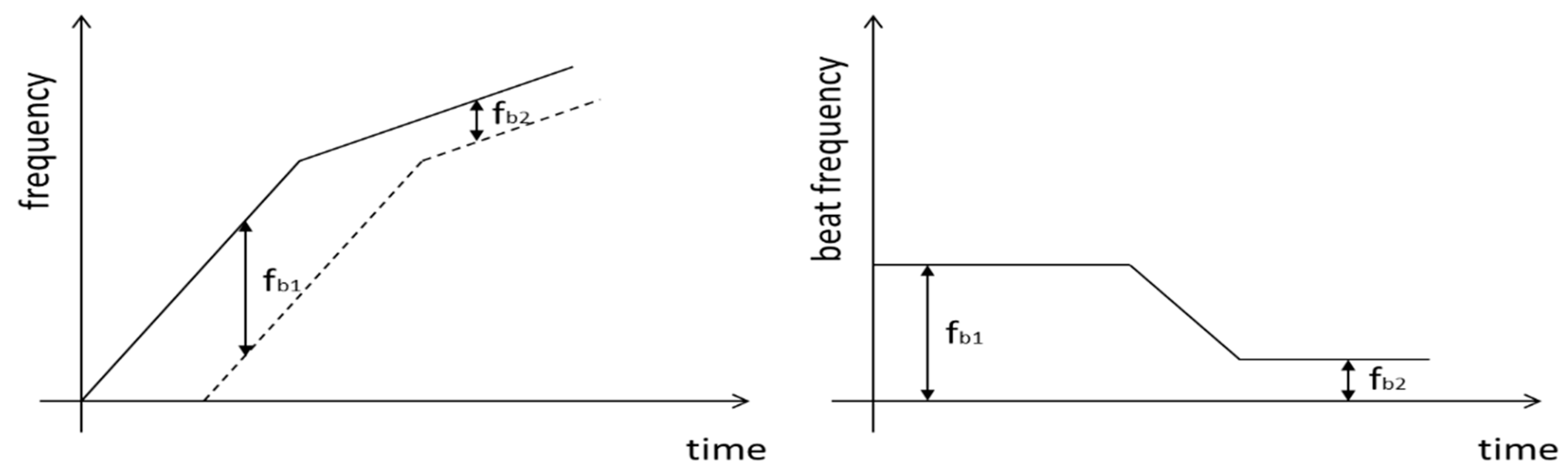
For FMCW radar, the linearity of the frequency modulation is critical for the accuracy of the outputs, as shown conceptually in Figure 2. That is, if the frequency modulation is not linear, the beat frequency for a point target will not be constant, and the range resolution will deteriorate. This limitation is a fundamental problem with the previous FMCW radar system. If the sweep bandwidth is increased, the range resolution improves. However, simultaneously, the total nonlinearity increases, and the range resolution degrades. Thus, the time variant of the beat frequency introduces a smeared frequency spectrum. Using a DDS device in ramp generation and replacing the voltage-controlled oscillator (VCO), which have been reported as the primary sources of nonlinearity in the FMCW system [25,26], is one method to improve Tomoradar’s linearity. Theoretically, the nonlinear characteristics of the frequency modulation module and the combined non-flat in-band response of all the RF components of the system generate nonlinearities in signal frequency. Although the non-linearity of the frequency modulation module is mitigated, the measurement should be calibrated to assure its accuracy. The calibration of profiling radar is also discussed in Hyyppä et al. [27].

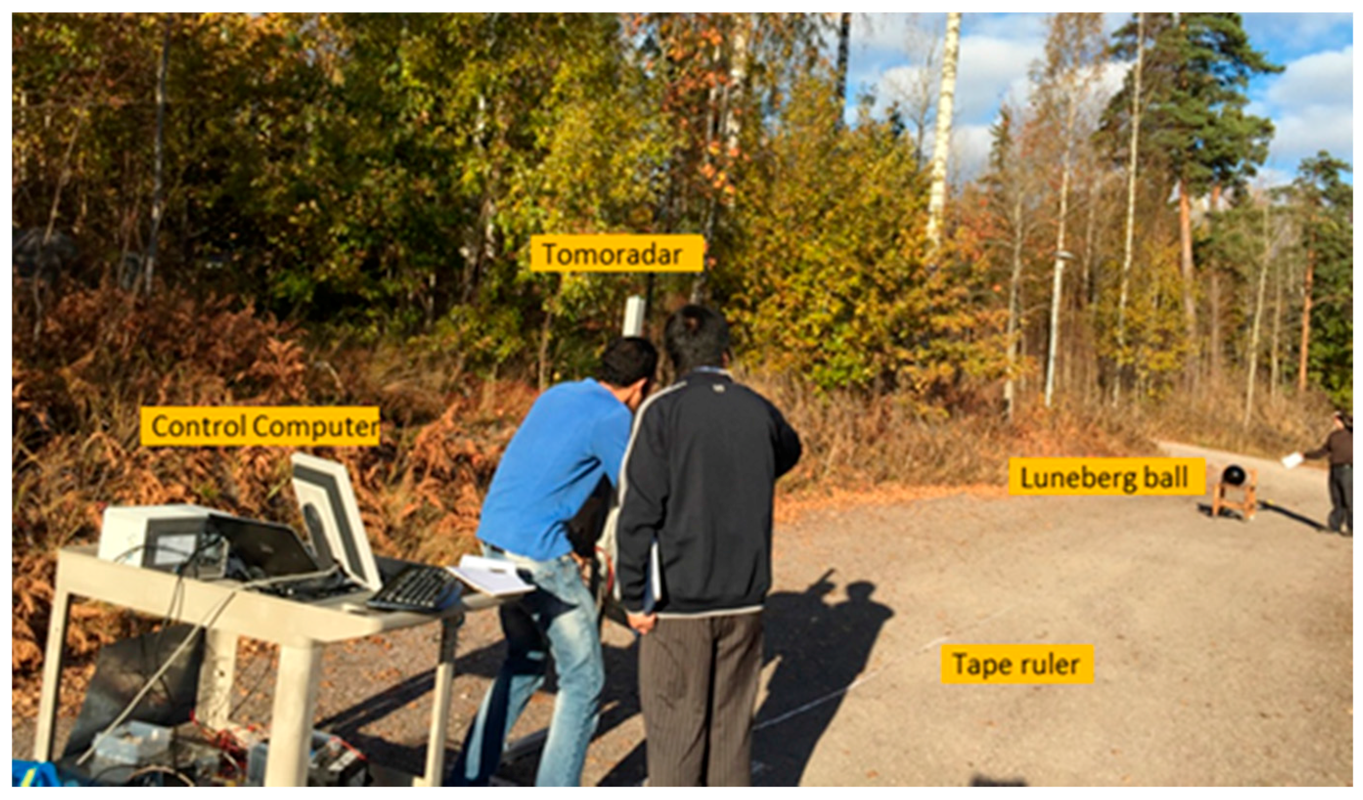
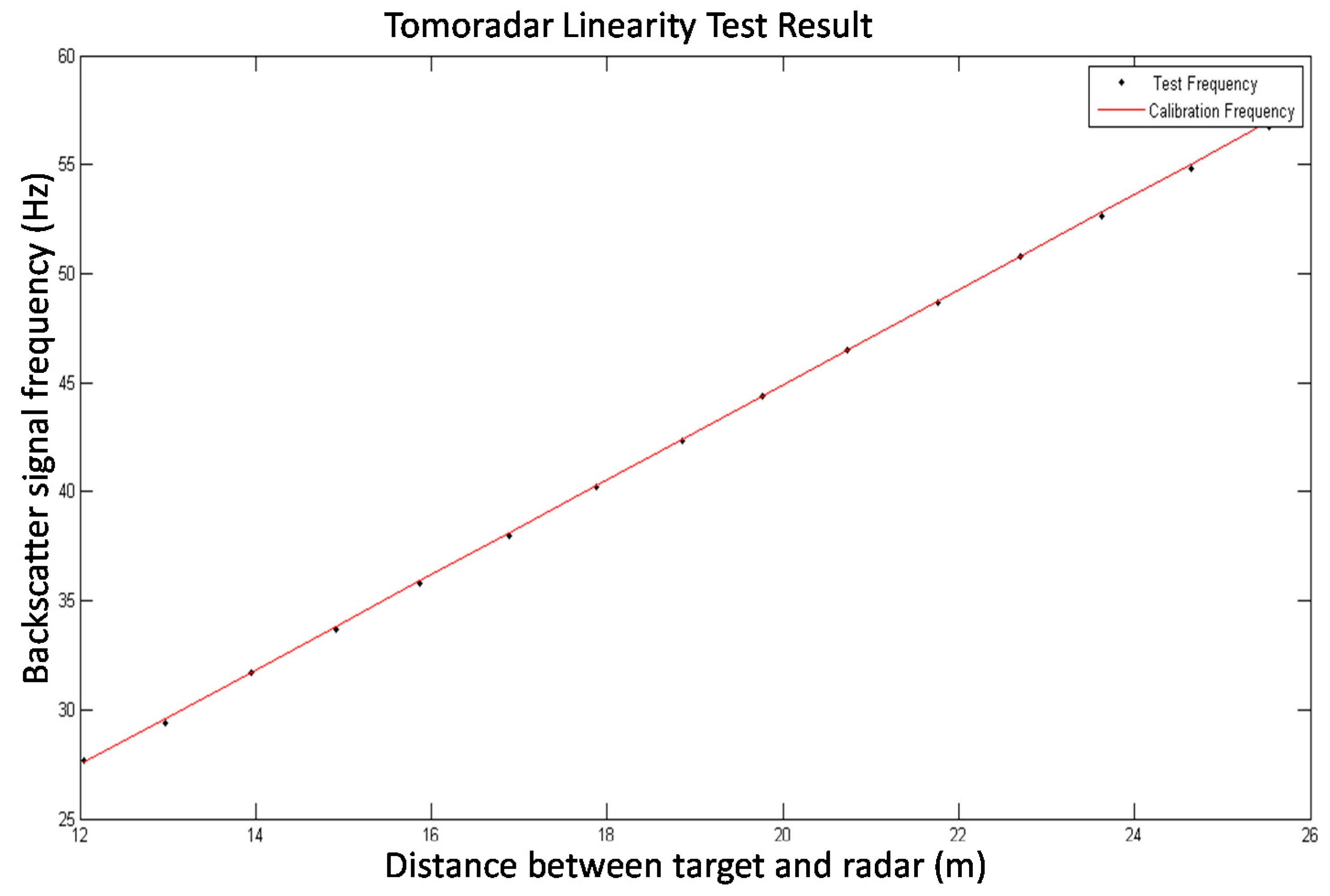
Based on the linear relationship, the range calibration was designed to probe a target at different positions using Tomoradar and to record the target backscatter waveform intermediate frequencies. In addition, the real distance between the target and Tomoradar was measured and then compared with the target range derived from the frequency. Eventually, a calibrated linear model was calculated. A 30 cm Luneburg lens (RCS = 100.35 m²) was used as a target and positioned on a wooden cart. Wood produces less backscatter signal, which was treated as noise in the experiment. A tape ruler was fixed between the radar and the target to offer an approximate range measurement during the test. As the experiment was conducted, the lens was moved along the tape ruler, and the real distance between the lens and radar was measured using a laser distance meter.

During the calibration, the distance from the radar to the lens increased from 10 m to 40 m in one-metre steps. The digitizer recorded the reflected IF spectrum for each step. By repeating the measurement at different distances, the effect of multipath propagation was decreased. Figure 3 presents the calibration arrangement and surrounding environment. Figure 4 shows the asymptotic fitting line between the measured frequency and distance. The relation between the true distance R and the measured intermediate frequency $f_{if}$ is as follows:

$$R=\frac{f_{if}-2.5893}{2.1707}$$

(7)

2.6. Post-Processing

The amplified horizontal and vertical polarized IF signals were digitized at a 2.5 MS/s sampling rate and streamed to a hard drive. FFT was performed in real time for part of the data for in-flight visualization purposes. However, these data were not saved. FFT was performed in post-processing at the same time as the frequency-to-distance calibration. For each DDS frequency sweep (i.e., profile), the GNSS IMU data were used to calculate the position and orientation of the profile. A digital elevation model (DEM) of the area acquired from ALS data or other techniques can be used to calculate the distance to the ground and the ground coordinates for each profile. These data can later be used as a reference when processing the profiles. They are also required when comparing the ALS and radar data. 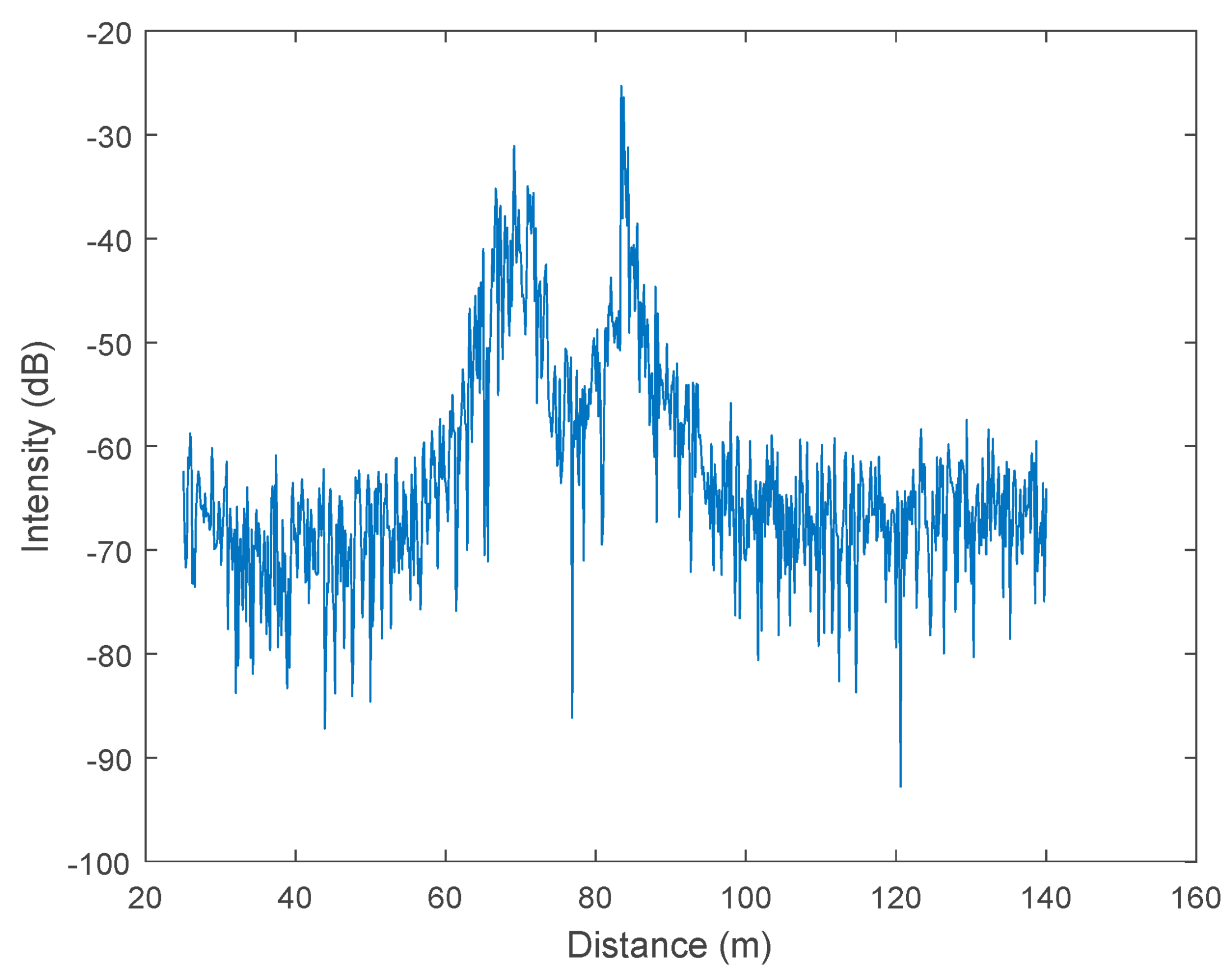Figure 5 presents a radar profile of a pine forest when the helicopter flew at approximately 85 m above the ground.

3. Field Test

3.1. Test Site

Evo is a test site located in southern Finland (61°19′N, 25°11′E). It is part of the southern Boreal Forest Zone and consists of approximately 2000 ha of primarily managed boreal forest. The dominant tree species in the area are Scots pine (Pinus sylvestris), Norway spruce (Picea abies) and birch (Betula sp.). Evo was selected because it is a popular recreation area, which distinguishes it from completely homogenous managed forests, and because it provides a cross section from natural to intensively managed southern boreal forest. The prototype Tomoradar was used to probe the Evo site in October and December 2015 and September 2016. The site was also surveyed by Riegl VQ-480-U laser scanner on helicopter platform on October 2015, the average point density is approximately 35 points per square meter. Thus, the ALS data for the same forest could be compared with the data collected using Tomoradar. The DEM of the Evo site was also collected at a 1 m resolution.

3.2. FGI-Tomoradar Data Collection

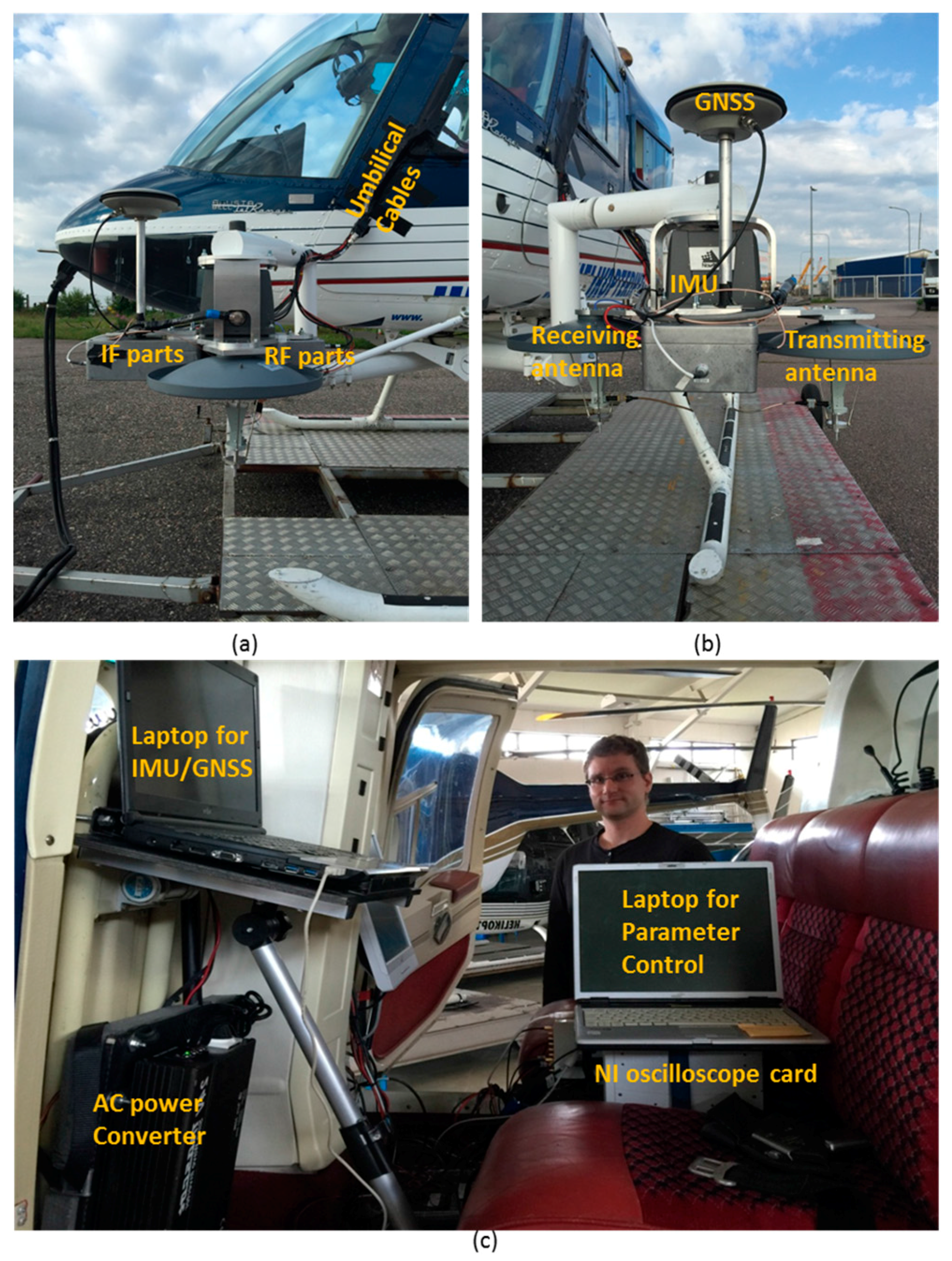
During the Tomoradar test, the RF and the IF units were installed on an arm of a Bell 206 helicopter with a 0 degree incidence angle (i.e., with the antenna pointing down). To shorten the length of the RF cables as much as possible for better signal quality (i.e., to reduce the internal reflections), the RF and IF units were installed on the bottom side of the frame on which the parabolic antennas were also installed. The IMU was installed on the frame’s top side, and the GNSS antenna was installed on a mast that was attached to the front of the frame (Figure 6a). Although the helicopter blocked part of the GNSS signal, the post-processed position results indicated that the effect of the blockage was minor. The digitizer, control computer and power unit in the cabin were connected to the RF and IF units by umbilical cables.

The digitizer can process the received IF waveform and present the FFT results in real time using a self-developed program. However, rather than the FFT results, it records all raw data at a 2.5 M sample rate. The data is processed in a post-processing way.

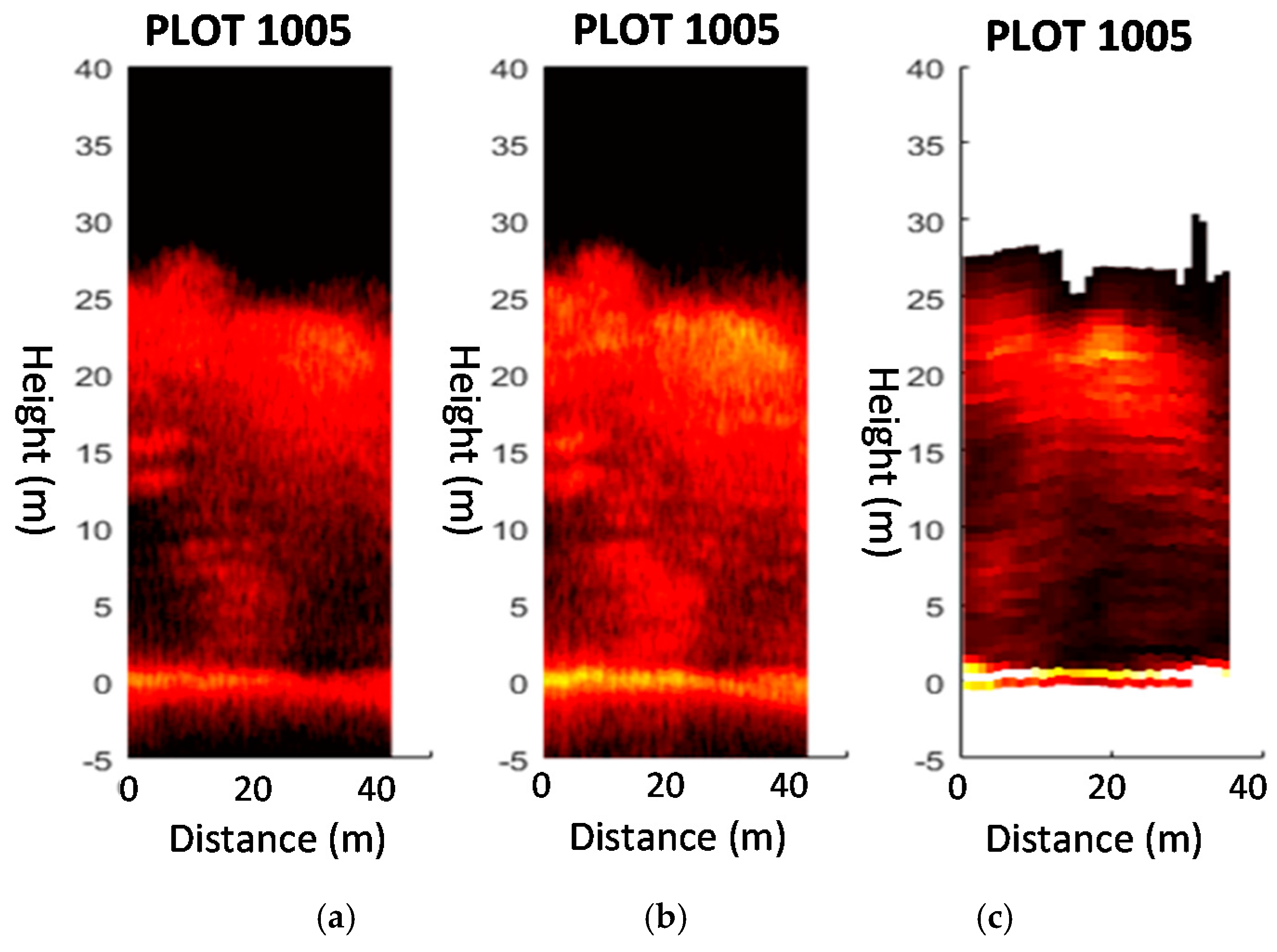
3.3. General Data Quality and the Calibration Results

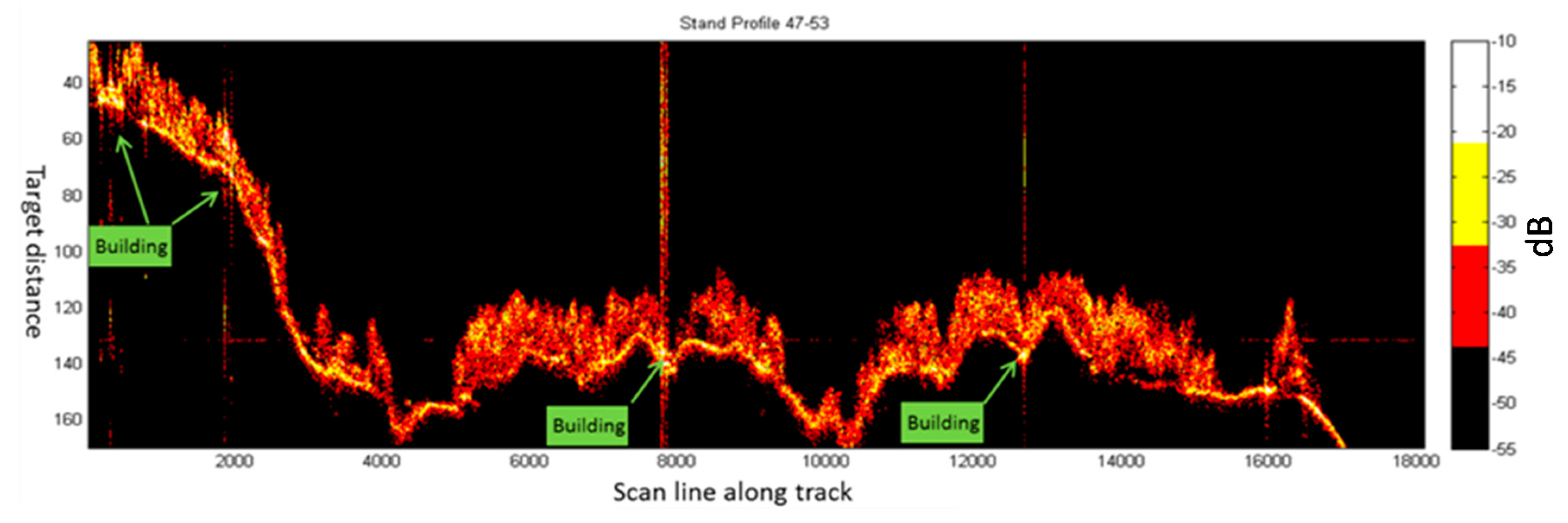
Figure 7 presents a stand profile created during the test. It can be observed that the system functions properly on all measurement ranges (10–150 m). The canopy structure is clear. It can also be observed that several saturation cases occurred during the test. The saturation was caused by echoes reflected by highly reflective objects, such as metal roofs measured perpendicular to the surface.

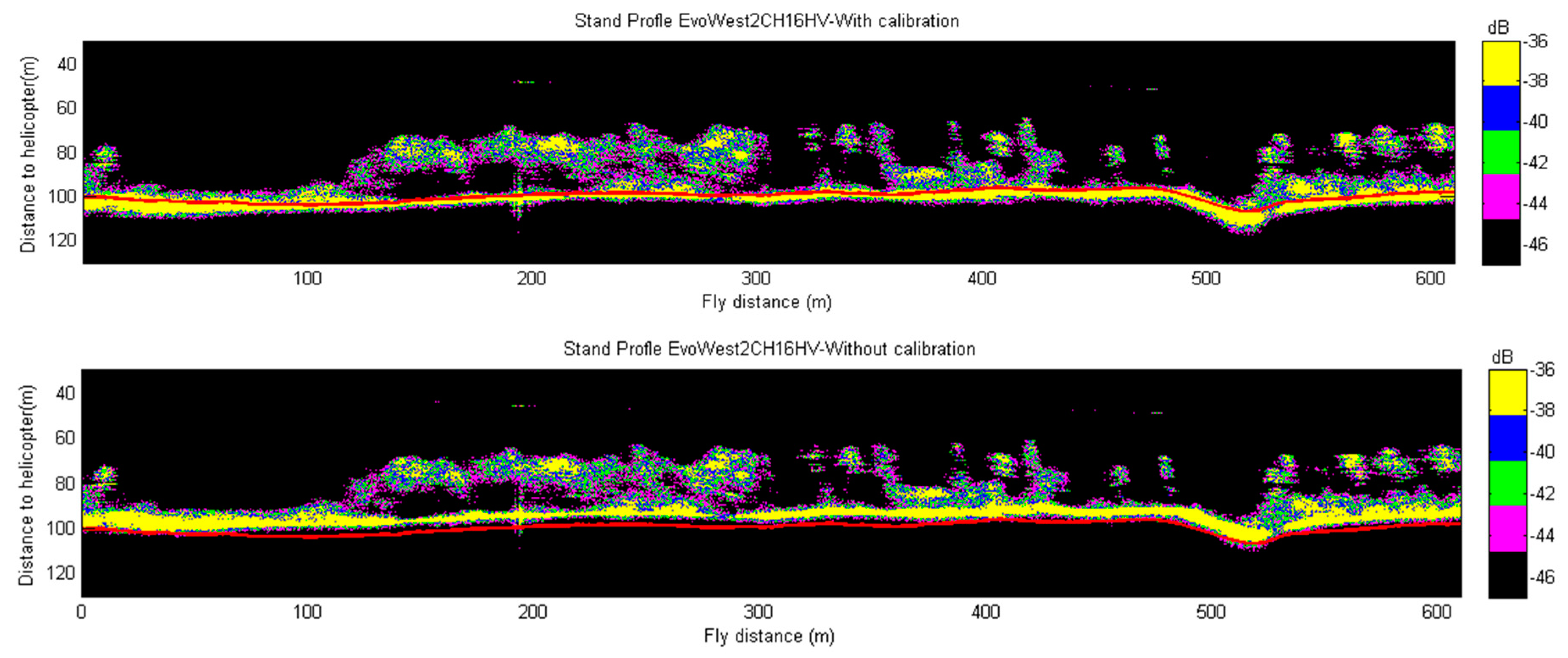
The range measurement of Tomoradar was calibrated using Equation (7). The results are presented in the top plot of Figure 8, where the red solid line indicates the ground level of the observed area extracted from DEM as a reference. In addition, the range without calibration is presented in the bottom plot in Figure 8 with same ground level. It can be concluded that the range error is calibrated by the range calibration method proposed in Section 2.4.

3.4. Ground and Canopy Information Extraction

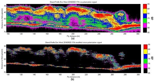
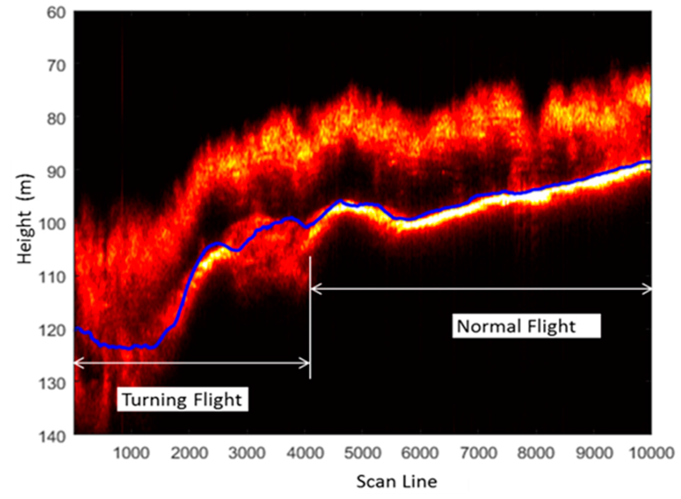
Since the Tomoradar was installed at a 0 degree incidence angle and the existence of forest gap, besides the canopy structure, the backscatter from underneath layers such as trunk, bush and ground can also be detected with Tomoradar. This procedure is critical for future measurements in areas in which a DEM is unavailable or the DEM resolution is inadequate. Even in presence of dense canopy, the ground reflection signal is strong and can be easily recognized. In this section, two test cases are investigated: the first case is that the helicopter turned when Tomoradar surveyed a mature forest with co-polarization mode in Figure 9; the second case is that Tomoradar data was used to process co-polarization and cross-polarization signals, Figure 10.

It can be observed from the Normal Flight segment in Figure 9. The blue solid line is the ground level reference extracted from DEM coincides with the ground reflection. However, when the helicopter turns, the ground reflection becomes blurred together with the forest canopy in Figure 9. When the helicopter was turning, the incidence angle changed from 0 degree to tens of degrees. Therefore, Tomoradar sees the increased attenuation of the forest and the number of multiple reflections are increased since there do not exist any canopy gaps as in nadir looking measurements. The bright signal in nadir measurements is due to canopy gaps, and they disappear between 10–30 degrees based on earlier FGI measurements. This topic is further studied in future studies.

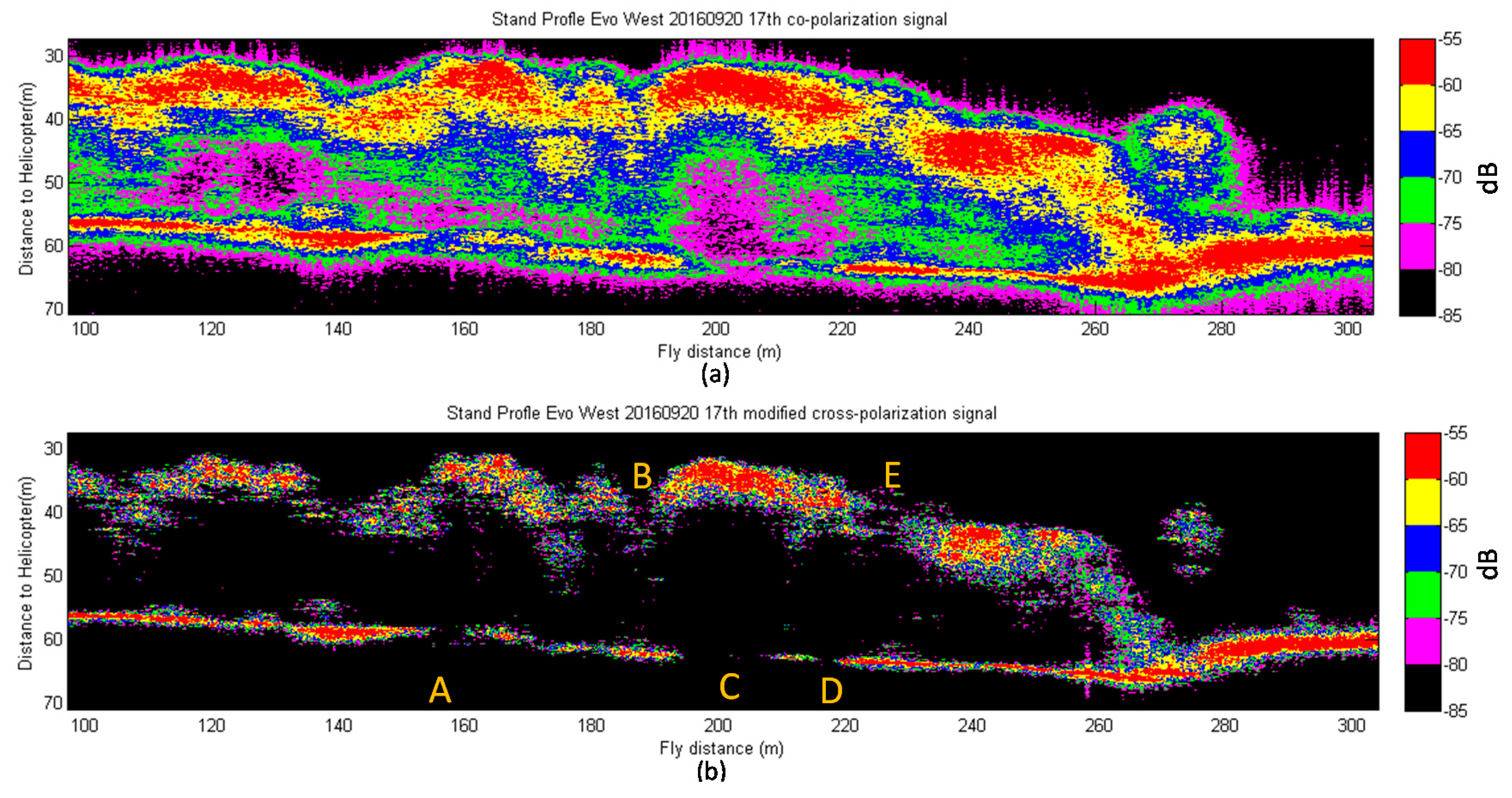
Figure 10 presents a case in which the co-polarization (HH) measurement and cross-polarization (HV) measurement of a stripe were simultaneously collected during the Tomoradar EVO field test. The following phenomena can be observed.

• The general reflection of co-polarization is stronger than cross-polarization.
• The Tomoradar can collect the profile information from tree canopy top to ground level through the branch and trunk both for co-polarization channel and cross-polarization channel.
• Strong cross-polarization could be observed in the top level tree canopy and ground level but not in branch and trunk section beneath the tree canopy since cross-polarization is caused by needles and small ground level features.
• Strong co-polarization could be observed also from tree canopy and ground level. However, the penetration depth for the co-polarization is deeper than cross-polarization mode since also branches are giving backscattering but not that much of cross-polarization.
• The ground backscatter is determined by various factors, such as:

  ◯

  Canopy gap: the backscatter is the strongest with larger canopy gaps, such as in sites B and E in both co-polarization and cross-polarization channels;

  ◯

  Canopy density: dense canopy may totally block the radiation from ground floor, such as in sites A, C and D. High canopy density results in high attenuation of ground signal. Dense forests having large number of needles seem to be more noticeable from the cross-polarized signal.

From the aforementioned observations, we can generally conclude that the microwave radiation propagation model in boreal forest is more complex than a homogeneous media. It is a function of canopy gap and canopy density resulting in attenuation. Penetration capability of Ku band profile radar is considerable stronger than its SAR counterpart, it can penetrate the boreal forest throughout from canopy to ground level, and collect the profile information both in cross-polarization and co-polarization modes. The structure under the tree canopy are more readily detected by co-polarization channel while the dense canopy structure are more noticeable in cross-polarization.

3.5. Comparison of Tomoradar Results with ALS Data

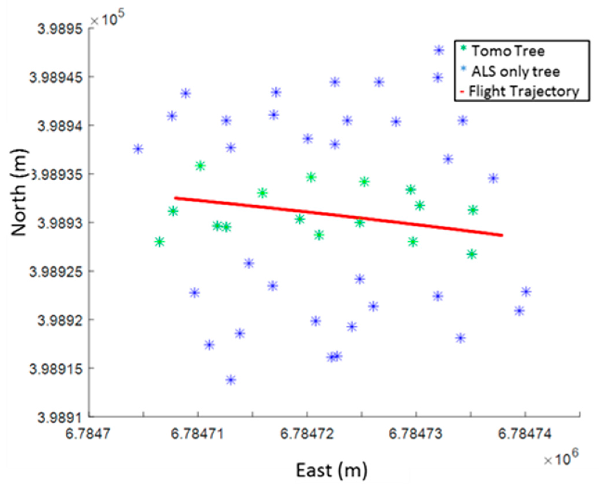
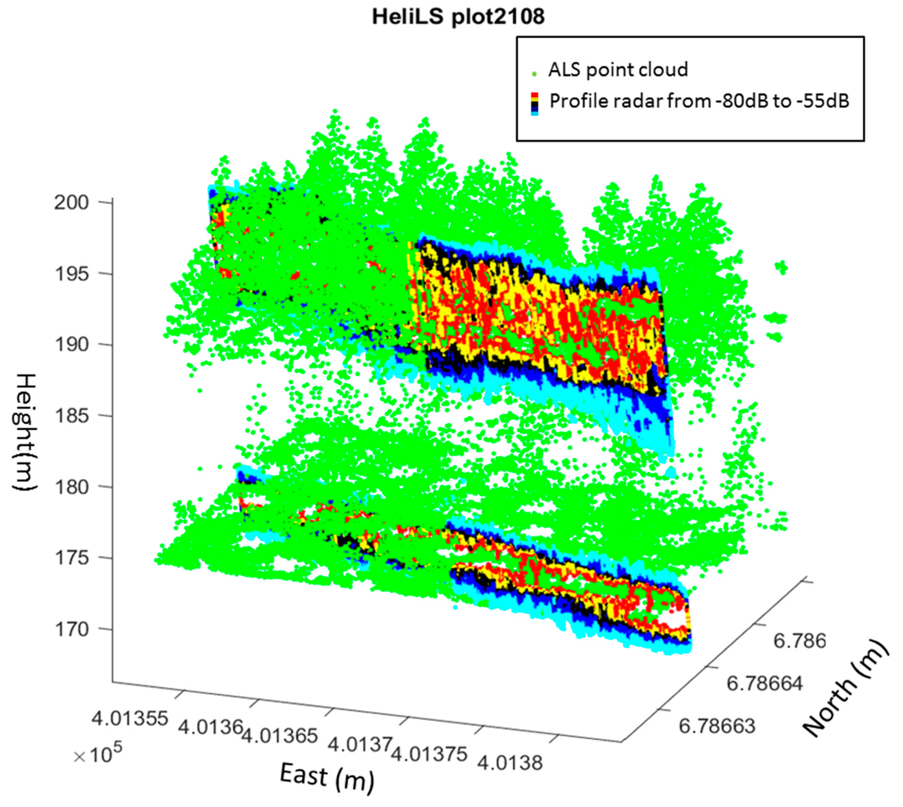
Since Tomoradar has no scanning mechanics, its FOV of 6 degrees is determined by the 3 dB beamwidth of the antenna. The ALS scanning angle is substantially wider. To compare the Tomoradar measurement with the ALS data, the tree canopy detected by Tomoradar should be compared with its counterpart in the ALS data. This type of registration problem can be resolved using the global coordinate measurements of the georeferencing system. Figure 11 illustrates and explains how to resolve the problem. In the figure, the helicopter’s trajectory during the test is presented as red solid line, which was measured using the georeferencing system with an accuracy better than 3 cm. The position of the tree was determined using a ground survey by total stations, whereby the position accuracy was better than 10 cm. The trees within the 6 degrees of the Tomoradar beamwidth footprint are represented as green asterisk marks in the picture, which of course can also be probed using the ALS system. The blue asterisk marks represent the trees that are only visible in ALS.

Since the instant FOV of the ALS is 0.3 mRad, the ALS footprint is substantially smaller than that of Tomoradar (0.03 m for ALS vs. 10.5 m for Tomoradar at 100 m altitude). The point cloud collected by ALS cannot be directly compared with the Tomoradar results. Thus, we propose an indirect method by generating a similar “IF spectrum” using the ALS point cloud.

If the flight altitude and DEM of the survey plot are known, the Tomoradar footprint can be calculated, the coordinates of the footprint cone can be determined, the ALS point cloud within the footprint cone can be selected and the height histogram of the ALS point cloud from the same observed area can be generated as radar data. In certain cases, normalization is required.

Figure 12 compares the radar-like results from Tomoradar and ALS. Since ALS and Tomoradar operate on different bands (i.e., ALS on near infrared) and Tomoradar on the Ku-band (14 GHz)), the results should not be identical but comparable because of the different physical nature of the sensing technologies. Because the incidence angle is 0 degrees, we only selected one cross-polarization and one co-polarization channel for the analysis. In Figure 12, we can observe a clear, dense canopy in the upper-right section of the tree canopy in three outputs, and the topography of the tree canopy in the upper layer is similar in the three outputs. The intensity of the cross-polarization results is lower than that of the co-polarization results for same target. After range calibration, the canopy height extracted from the Tomoradar results is comparable with that of ALS. However, in the Tomoradar data, more detailed structures under the canopy are disclosed than in the ALS data due to Tomoradar’s penetration capability.

After geocoding the Tomoradar and ALS measurements in Evo test field, some qualitative results could be observed (and example plot in visualized in Figure 13):

(1)

The tree top of Tomoradar data (light blue on the top) is lower than the tree top of ALS measurement. The major reason is the better penetration of Ku-band signal into forests. The larger FOV of Tomoradar also affects the analysis. The numerical values are analysed in more details in future studies.

(2)

The profile depth (colourful profile data within the green point cloud generated by ALS) of Tomoradar on canopy part is proportional to the canopy depth of the ALS measurement.

(3)

Combining topography information collected by laser scanner and density information unveiled by profile information archived by Tomoradar, a more composite forest model can be generated than any single sensor can output, such complex model suggests better understanding of how RF signal propagates in boreal forest, which assists the post processing research of SAR signal.

4. Conclusions

An UAV-based profiling radar for forest research was depicted. Using a helicopter field test, the developed system was analysed against Riegl VQ-480-U laser scanner. Using high-quality georeferencing system, we measured radar profiles (i.e., waveform) from forest canopies and compared them with ALS data. The results showed good agreement of radar and lidar signal from forest structures. However, future research is needed to better understand the characterizing the role of canopy gaps and radar attenuation in the Ku-band in forest canopy as a function of forest-stand attributes. Such characterization could not be conducted in the early studies of profiling radars due to a lack of georeferencing technology. Thus, the objective of future research on the new system is to improve our understanding of laser and radar beam interaction in forest canopy. The following preliminary conclusions were drawn:

• The Tomoradar can collect the profile information from tree canopy top to ground level for both co- and cross-polarizations.
• Strong cross-polarization signal, which is at the level of co-polarized return, can be detected at dense coniferous tree tops due to volume backscattering of the needles at Ku-band.
• Height of canopy is underestimated due to penetration of Ku-band signal into forests.
• The canopy return is a combination of canopy gaps and density of canopies affecting attenuation of canopies.