1. Introduction
Canopy cover information is essential for understanding spatial and temporal variability in vegetation biomass, local meteorological processes and hydrological transfers (i.e., energy in heat variations, gas and water) within vegetated environments [
1]. Canopy cover has been monitored via satellite and airborne remote sensing technologies for decades, providing information on vegetation and biomass conditions from local (100’s of km
2) to global scales [
2,
3,
4]. However, the passive nature and/or low resolution of satellite sensors have restricted our ability to simultaneously map canopy structural attributes over large areas and at the tree crown level [
5,
6].
The use of Airborne Laser Scanning (ALS) for deriving canopy cover indices has been demonstrated at forest stand scales by many [
7,
8,
9,
10,
11,
12,
13]; however, due to costs and sampling logistics, ALS acquisitions are typically limited in spatial extent. In contrast, the Geoscience Laser Altimeter System (GLAS), which previously operated (2003–2009) onboard the Ice, Cloud and land Elevation Satellite (ICESat), has the potential to retrieve canopy cover indices at near global scales, but has not demonstrated the same success as ALS to date. The large-footprint continuous waveform nature of GLAS data has been suggested to be sensitive to apparent canopy and ground surface reflectance values; that is, canopy returns reflect stronger or weaker than the ground [
14]. Radiative transfer analysis partially corroborates these findings [
15], but suggests a greater influence is caused by waveforms being more sensitive to within canopy scattering events, which may lead to less energy irradiating the ground surface [
16]. Further compounding the misinterpretation issues, the non-uniform footprint energy distribution effectively irradiates targets with higher intensity at the footprint centre. This systematically alters the footprint backscatter signature, which is embedded in the location and amplitude of peak(s) in the waveform profile, the analysis of which allows the retrieval of Gap Fraction (GF). Given a non-uniform energy distribution, retrieved GF is expected to be different to reality due to artificially enhanced illumination at select locations within the footprint (energy distribution dependent), whereas a uniform energy distribution (similar to that of the Sun) is expected to alleviate this issue.
A practical solution is to scale waveform ground or canopy returns to account for waveform reflectance differences; however, this remains an active area of research. To date, Lefsky et al. [
14] demonstrated that scaling the waveform ground return by a factor of two resulted in more highly correlated estimates of Fractional Cover (FC) with respect to ALS data for the relatively small footprint sensor: Scanning Lidar Imager of Canopies by Echo Recovery (SLICER). This approach was adopted by Luo et al. [
17] for GLAS with encouraging results. However, by design, the application of such a scaling factor is not tolerant of any deviation attributed to variable environmental characteristics from those for which it was specifically derived, i.e., the deciduous forests of eastern Maryland, USA. Tang et al. [
18] scaled Laser Vegetation Imaging Sensor (LVIS) waveform data by field acquired ratios of vegetation and ground reflectance values from spectroradiometers to refine estimates of GF. Whilst this applies a more empirically-based method to estimating canopy cover, the need for extensive field data limits the spatial reach of such analysis. As follow-up studies, Tang et al. [
19] and Tang et al. [
20] built on previous findings and employed a recursive algorithm to retrieve estimates of Leaf Area Index (LAI) via refined GF estimates from GLAS; however, this method required the use of some locally applicable initial conditions by which scaling factor outputs were governed (i.e. expected minimum and maximum values). Previous studies fail to meet the need for correcting waveform-based canopy cover indices by both empirical and independent means at large scales. Furthermore, with the view of large-scale application, the derivation of a scaling factor based on large-scale measured/estimated predictor attributes is required in order to make waveform scaling viable at large scales; a key focus of the current study.
GLAS data are currently the only near global active (i.e., capable of penetrating the canopy to retrieve within-canopy information) laser data available, and the need to identify which attributes are best suited to spatially scale GLAS estimates of canopy cover is pertinent, as future missions (e.g., NASA’s Global Ecosystem Dynamics Investigation Lidar; GEDI) will provide similar data. Establishing robust methodologies for deriving spatially large-scale parameter estimates by current data will not only be applicable to future data, they will allow contemporary products to be established, which will offer a basis from which large-scale monitoring investigations can be conducted.
In the current study, a method for the general application of scaling factors at large scales is developed and tested for sensitivity against predictor attributes. The sensitivity of terrain and vegetation characteristics are investigated as a function of the difference in canopy GF estimates from ALS and GLAS in order to identify which attributes best predict a difference between sources of GF estimation. This will accommodate spatial up-scaling, allowing the use of imputation techniques, such as Random Forest (RF) [
21], to map GF continuously at continental scales in future studies. Furthermore, the potential value of restricting GLAS data to an optimal subset, as identified by Mahoney et al. [
22], for model training purposes is investigated against training models with all available data. GF estimates are identified as a value-added output in this study, as they provide a basis for estimating the Leaf Area Index (LAI) using the Beer–Lambert law assumptions (not studied here, but the basis of ongoing research).
2. Materials and Methods
2.1. Discrete Return ALS Data
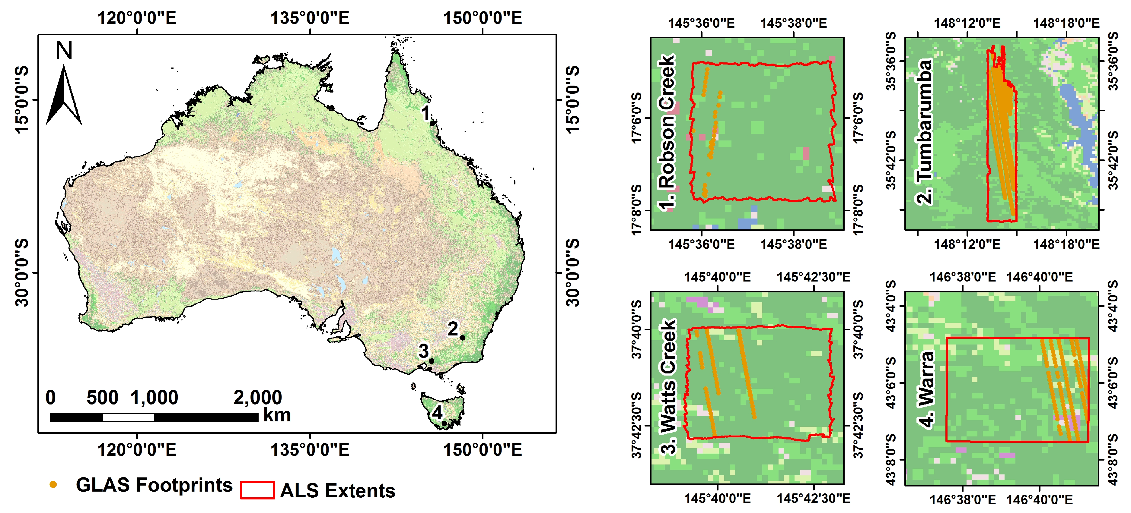
Three Terrestrial Ecosystem Research Network (TERN) supersites and a single independent site in eastern Australia are employed in the current study (
Figure 1). Each site is forested and has been surveyed with ALS and GLAS data. Individual ALS surveys were acquired using a Reigl Q560 by Airborne Research Australia (ARA) during the Southern Hemisphere summer and/or fall seasons of 2009, 2012 and 2014.
Robson Creek (17.106°S, 145.622°E) is located approximately 25 km southwest of Cairns. The forest exhibits moderate relief and ranges from complex mesophyll vine forest to simple/complex notophyll vine forest with increasing elevation to the north. ALS data were acquired during September 2012 with a mean point density of 5–6 points per square meter (ppm
2). Watts Creek (37.692°S, 145.684°E), located 70 km east of Melbourne, is an old-regrowth open forest dominated by Eucalypts over complex terrain. ALS data were acquired with a mean point density of 5–6 ppm
2. Warra (43.106°S, 146.657°E) approximately 60 km southwest of Hobart, Tasmania, is a cool, temperate wet forest biome over moderately complex terrain. The site consists of moorland, temperate rainforest, riparian and montane conifer forest and shrubs. ALS data were acquired during May 2014 with a mean point density of up to 25 ppm
2. Tumbarumba (35.686°S, 148.234°E) is approximately 120 km southwest of Canberra. It is a Eucalypt-dominated, moderately open forest with complex terrain [
23,
24]; ALS data were acquired during November 2009 at a mean point density of 5 ppm
2. This site is not to be confused with the TERN site at the Tumbarumba research station, the site employed here is located approximately 7 km east of the research station, but the vegetation and terrain characteristics observed at the research station are still applicable. This location was strategically selected as a study site due to overlap with numerous GLAS footprints.
2.2. GLAS Data
The ICESat/GLAS land data (GLA14 data product), Release 33 [
25,
26], are employed in the current study. GLAS data are continuous waveforms; the returned echo pulse forms an energy profile, which is a function of surfaces encountered during transit, such as vegetation and/or ground surfaces [
27,
28,
29]. The returned energy profile is fitted with up to six Gaussians as described by Duong et al. [
30], the sum of which defines the ‘model alternate fit’ return pulse.
For this study, only GLAS data acquired within forested regions are employed, where Australia’s forest regions are delineated by the tree classes of the National Dynamic Land Cover Dataset (DLCD): closed, open, sparse and scattered; technical details of the DLCD can be found in Lymburner et al. [
31]. To further maintain GLAS data integrity, footprints that were saturated upon detection and/or experienced cloud cover whilst in transit are excluded from analysis. Additionally, footprints that exhibit an absolute difference between GLAS and Shuttle Radar Topography Mission (SRTM) elevation estimates >8 m are also removed [
32]. Post filtering, a total of 457 GLAS footprints are available for analysis; this reduces to 175 after filtering by the ‘optimal’ criteria, i.e., high energy (>28 mJ) Laser 3 acquisitions during summertime (cf. Mahoney et al. [
22]).
The employed GLAS data (post filtered and optimal) exhibit a temporal range from February 2004–October 2008, where Southern Hemisphere summertime is defined from October to the subsequent March. Little effect on the outcome of this analysis is expected from the temporal disparity between GLAS and ALS data as GLAS waveform profile portions (reflections from canopy and ground) are refined with respect to ALS data regardless of acquisition time. Temporal disparity will likely play a greater role when attempting to model GF from refined GLAS data for specific time periods (with respect to vegetation phenological state); i.e., ALS data will need to be available for that specific period in order to allow GLAS model development.
2.3. ALS Gap Fraction
A number of methods exist for deriving GF from ALS point cloud data. A simple method that uses return ‘intensity’ is selected here. This selection was made on the basis that intensity has been shown to be more directly related to GF than return count [
1,
13]; furthermore, intensity ratios are more analogous than return ratios to the energy distribution encountered with GLAS data. GF is defined as the ratio of the sum of intensities from all returns (first, intermediate and last) that exist between the canopy top and 2 m above the ground (
) and the sum of intensities from all returns between the canopy top and the ground itself (
; Equation (1); Hopkinson et al. [
1]). Estimates of GF are calculated directly from the portions of the ALS point cloud data that are within the boundaries of unique GLAS footprints. This method allows a direct comparison of ALS estimates of GF to GLAS equivalents.
Further fortification of this methodological selection is supported by the high correlation demonstrated (R
2 = 0.92) between this ALS product and field measured GF via Digital Hemispherical Photographs (DHPs) in mature and regenerating mixed wood plots [
13]. This method was up scaled and applied to 7 Canadian boreal sites where similar high correlation was also demonstrated (R
2 = 0.77) [
1].
2.4. GLAS Gap Fraction
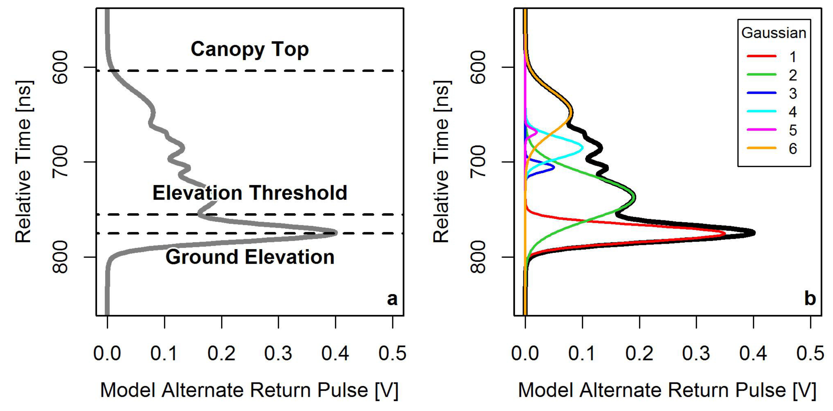
The derivation of GF from waveform data (such as GLAS) is analogous to that of the point cloud intensity method described in Equation (1) with minor modification. Where a ratio of summed intensities is noted, waveform GF is calculated from the ratio of summed energy from particular portions of the profile, such as those reflected from the ground and/or vegetation surfaces only. In particular, GF is calculated as one minus the ratio of the sum of the returned energy between the canopy top and 2 m above the ground, and the sum of energy between the canopy top and the ground (
Figure 2a). The waveform equivalent of Equation (1) is given by Equation (2), where energy (
ϵ) replaces return intensity (I).
Whilst simplistic in principle, the large footprint nature of GLAS often presents challenges in locating the true ground elevation. This becomes particularly challenging when attempting analyses over complex terrain [
33]. In an attempt to mitigate the influence of complex terrain, we employ the method of Rosette et al. [
34] to locate the ‘ground’ in returned GLAS waveforms. This method makes use of the (up to 6) fitted Gaussians that form the model alternate return pulse, where the ground is considered to correspond to the centre of the Gaussian that exhibits the greatest amplitude of the two that are least elevated within the waveform (
Figure 2b).
2.5. Gap Fraction Scaling
The literature suggests that a scaling factor applied to either the ground or vegetation portions of waveforms will yield more coherent results with respect to ALS equivalents [
35,
36]. GF estimates from waveforms can be broken down into energy contributions from canopy and ground components and be represented with the necessary scaling factor (f) by Equation (3).
As GF estimates from ALS data have been demonstrated to yield high correspondence with field acquired data, these estimates are assumed to be correct. By this assumption, and the fact that ALS estimates of GF (
) can be represented by Equation (3) (i.e.,
when f is 1), Equation (3) can be arranged to make f the subject (Equation (4)). This offers a means of scaling waveform estimates of GF to ALS equivalents by physical observations, i.e., GLAS measured canopy and ground components.
Scaling factor values are predicted (from a minimum of 0.25 in 0.25 intervals) for each GLAS footprint based on predictor attributes via a novel approach that utilizes RF regression algorithms; however, the knowledge of which attributes will produce the best predictive results is not a priori known. As a result, all predictor attributes are initially tested, and predictions are refined based on the importance assigned to each attribute by the RF algorithm. RF scores the importance of each variable by the increase in the mean of the error of a tree in a forest when the observed values of this variable are permutated in the Out-Of-Bag (OOB) samples; see Genuer et al. [
37]. As the importance measures assigned by RF are subject to the data selected to train the RF model, the order of variable importance may change if model training is repeated. In order to form a more robust estimation of which attributes scaling factors are most sensitive to, an independent analysis of attribute importance is performed also (methodology described below).
2.6. Predictor Attributes
As a finite coincidence is observed between ALS and GLAS data, it is not possible to map scaling factors and refined estimates of GF to individual GLAS footprints beyond ALS extents without the use of imputation algorithms. Such algorithms require the use of predictor attributes to predict a response; the more suitable the predictor data, the better the expected response (with respect to overall accuracy). Pre-empting the use of the scaling factor methodology at large scales, the sensitivity of the scaling factor is investigated with respect to 13 environmental attributes for possible use in imputation (
Table 1). It is important to note that each predictor attribute was resampled to the smallest common resolution (250 m in this case) among the available predictors. Additionally, the variability in the predicted scaling factors is gauged against two GLAS instrument attributes: laser campaign and footprint eccentricity, to identify if GLAS energy losses were consistent during its operational lifetime.
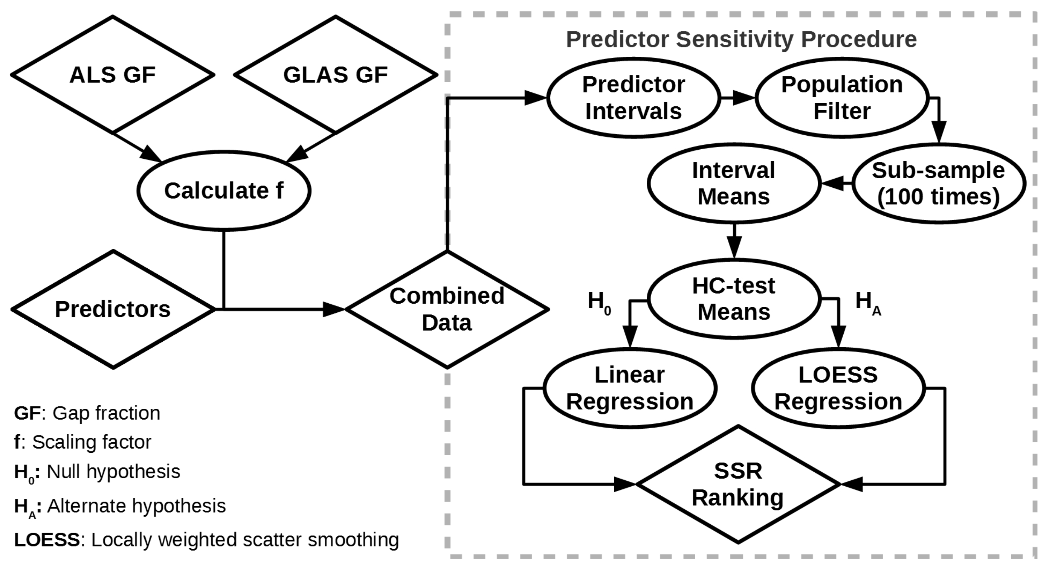
In order to reliably indicate if the GLAS scaling factor is sensitive to any of the 13 tested attributes, each attribute was split into intervals, where each interval exhibits a variable sample size. The largest common denominator of samples was selected without replacement from each interval, thus forcing each interval to be of the same sample size when analysed. Additionally, to avoid small interval sample sizes and under sampling bias effects, any intervals with <10 samples were excluded from analysis. To avoid any further bias by randomly sampling from each interval only once, the previously described process was repeated 100 times per attribute. This yields a more comprehensive and robust attribute data distribution across each interval.
The mean scaling factor required per subsequent intervals (per attribute) is analysed for linearity via a Harvey–Collier (HC) test for linearity [
46] and fitted with a linear regression model if the mean of the recursive residuals did not significantly (
α = 0.95) differ from zero. Rejection of the hypothesis of no significant difference of the recursive residuals from zero results in the execution of local polynomial regression fitting [
47]. The Squared Sum of fitted model Residuals (SSR) is assessed to yield an independent measure of variable importance. Throughout the regression analyses, mean values of f are not regressed against attribute interval values, but rather against a scalar that ranges from 1 to the number of valid (>10 samples) intervals. This allows for analytical consistency between numerical and categorical attributes, where the latter would otherwise exhibit some unordered category corresponding numerical code that may alter the magnitude of the calculated SSR, thus potentially changing the importance of certain attributes. This independent measure of variable importance is favoured over that built into the RF algorithm as RF importance measures are subject to the RF training data, which varies with model training repetition; hence, the order of variable importance may also vary. A general workflow of obtaining SSR information for ranking predictor importance independently is illustrated in
Figure 3; note that this workflow assumes calculations of ALS and GLAS GF.
2.7. Gap Fraction Comparisons
ALS estimates of GF are directly compared with spatially coincident, unscaled, GLAS waveform equivalents for all data, defined as ‘controls’. This yields a baseline against which comparative improvements or losses, via the application of scaling factors, can be assessed. Scaled estimates of GLAS GF are based on Equation (4), where f is predicted for each footprint via RF imputation where the RF technique was selected, as it is well documented and robust; however, the existence of other techniques for potential use should be acknowledged. Two sets of scaling factor predictions are made via RF: the first trained using all available GLAS data (coincident with ALS data), the second using GLAS data that are high energy (>28 mJ) Laser 3 footprints acquired during summertime only (as per Mahoney et al. [
22]). This restriction is imposed to investigate if such filters yield optimal results for GLAS GF estimates and are not only applicable to GLAS estimates of canopy height.
The RF algorithm is a decision tree ensemble technique employed in regression form here, where a total of 75% of a parent dataset of corresponding response (scaling factor) and predictor information is randomly sampled, defined as the ‘training’ set. The training set is used to grow a ‘tree’ of nodes, where a number of predictors are sampled and split via a threshold at each node to maximise information gain or Kullback–Leibler divergence [
48]. Node creation is repeated until information gain becomes negligible, thus producing a ‘leaf’. The training data selection and tree growth process is repeated 500 times, forming a ‘forest’ and trained RF model. In order to retrieve predictions from the trained RF model, each line of predictors (of the same format as the trained model) is processed through the previously created 500 trees. The pathway taken to a single leaf per tree is determined by the value of predictors sampled at each node and their values relative to the previously trained node thresholds. The mean of the leaf values obtained from each tree is taken as the final predicted output of the model.
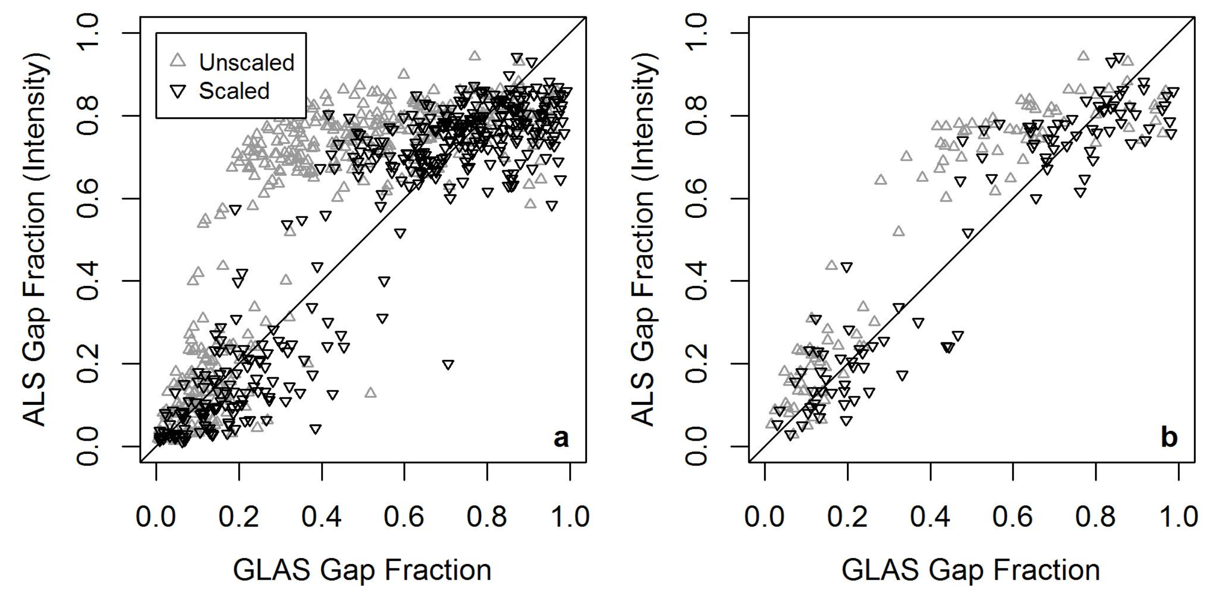
The direct comparisons of unscaled and scaled estimates of GLAS GF with ALS equivalents are quantified via a set of model summary statistics: root mean squared error (RMSE), the coefficient of determination (R2), fraction of predictions within a factor of 2 of observations (F2), fractional bias (FB) and mean prediction bias (). The difference in model summary statistics is noted between ALS and unscaled GLAS estimates of GF for all available GLAS data and the optimal subset. This comparison was also performed for two forms of scaled GLAS estimates of GF. The first set of refined GLAS GF estimates was modified based on predictions of f made from an RF model trained via all available GLAS data, where the second predictions of f were made via an RF model trained using the optimal GLAS subset only. The percentage difference of each summary statistic is calculated between unscaled and scaled GLAS GF estimates for all and the optimal datasets. Assessing the greatest accuracy gains between all and optimal datasets helps to identify if the restrictions of the latter are worth imposing for predicting large-scale estimates of GF across Australia.
It is important to note that predicted scaling factors made for all data are not expected to exhibit any ‘tuning’ bias even though the same data was used in RF model training. In the training process, RF grows numerous ‘trees’ (in this case, 500), each from a random selection of 75% of all available data. During the prediction process, each ‘tree’ provides a modelled response (500 in total) given the same predictors. The mean of all outputs from all ‘trees’ is taken as the final modelled response, thus negating any possible data ‘tuning’ bias.
4. Discussion
GLAS waveforms require scaling in order to retrieve accurate estimates of GF. This is a legacy of the non-uniform energy distribution with which the sensor illuminated its targets and suggested differences in reflectance values between vegetation and ground surfaces [
14,
35]. In the novel approach to predicting scaling factors for unique GLAS waveforms based on other remote sensing data products, soil phosphorus and nitrogen contents were identified as two of the most important attributes for scaling factor predictions, suggesting that soil mineral contents are key in influencing the density of vegetation canopies. Furthermore, it is possible that soil texture and colour may vary as a function of these variables also, thereby influencing soil reflectance properties. Vegetation height ranked second most important overall; this is somewhat expected in a forest environment (i.e. considering trees only), although caution is expressed, as this relationship may degrade with the inclusion of additional vegetation, such as shrubs, which can be short, but exhibit high cover densities. The Vegetation Cover Index (VCF) ranked fourth most important, which is a trivial connection between vegetation cover indices. Finally, slope is ranked as fifth most important, indicating that canopy density becomes limited with the vegetation’s ability to anchor itself, although this is expected to be somewhat species dependent.
With respect to large-scale derivations of GF via the presented waveform scaling methodology, the use of the five identified most important attributes is expected to be paramount; however, the need for attribute pre-selection will be a function of the selected imputation technique. For example, if RF were to be employed, the a priori identification of the most important attributes becomes somewhat irrelevant as RF is capable of selecting which attributes contribute most to yield the most accurate model. Conversely, when employing other techniques, such as kNN, the selection of an optimal set of predictor attributes is of great importance in the context of overall model accuracy [
49]. In such instances, the use of the presented attribute pre-selection analysis is advocated in order to identify attributes that best characterize the prediction/response variable. In the case of RF techniques, attribute pre-selection can still be applied in the pursuit of a parsimonious model, that is, computational processing time is reduced at the cost of marginal losses in overall accuracy. Therefore, by accepting this compromise, models can be applied over large scales with increased efficiency by a priori removing attributes that contribute little to the model; an approach already advocated by McRoberts et al. [
49]. However, in the case that a truly parsimonious model is desired, it is suggested that future studies filter predictor attributes that exhibit strong correlation with each other in order to maximise computational efficiency.
The presented attribute pre-selection methodology focussed on the identification of most important attributes for scaling GLAS estimates of GF by analysis of physical relationships only, i.e., neglecting relationships formed by complex interplay in statistical algorithms (such as RF). Such analysis was favoured as knowledge of the relationship between the environment and f is required to understand why f is an inherent requirement when attempting to obtain GF from GLAS (or any waveform system) data. The identification of these attributes will allow a better physical understanding of how such attributes contribute to how f varies as a function of landscape subtleties; this is otherwise unobtainable by sole reliance on statistical ensemble models. The quantification of such physical understandings is not pursued in the current study as the primary objective is to demonstrate a proof-of-concept for refining initial GLAS GF estimates as a function of ALS data. It is acknowledged that the same set of most important attributes could be identified via RF importance measures provided all attributes were employed in model building; however, without additional analysis, a physical understanding of why these were identified would not be known.
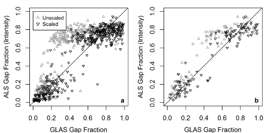
Even based on the relatively small ALS-GLAS coincidence noted here, the improved correspondence of GLAS results to ALS equivalents is evident. However, it is noted that GLAS-refined GF in
Figure 5a, and
Figure 5b are more outlying than unscaled GLAS GF equivalents; this is a somewhat expected result based on the inherent inability of RF to predict extreme values. This is due to RF prediction values being the mean of all ensemble results, which by definition will be less than the maximum and/or (above average) outlying prediction results, which are expected to occur minimally in the ensemble results. Modifications to the RF procedure have been attempted in order to mitigate this issue but at the cost of overall prediction accuracy [
50]. Furthermore, as a consequence of little coincidence, few GF data are available between 0.4 and 0.7; hence, any predictions made in this region are expected to exhibit greater uncertainties. Such a gap in results requires additional (coincident) ALS and GLAS data to validate any GF predictions made in this range. Given the increasing availability of ALS data globally, this may be achieved elsewhere across the globe, although any calculations made elsewhere will likely be subject to vastly different environmental characteristics and vegetation species to those noted in this Australia-centric study, which may require a new sensitivity analysis be conducted. Additionally, with increasing ALS data availability, the current methodology for scaling GLAS waveforms is pertinent as initial model training requires scaling factors be determined in areas of data coincidence. With increased ALS-GLAS data coincidence, uncertainties in scaling factor predictions are expected to decrease.
It is important to note that the predictor sensitivity results presented in this study are valid at 250 m spatial resolution only, but are expected to be applicable at large geographies, particularly Australia-wide or even globally. However, it is important to note for the latter that applicability will depend on the availability of similar predictor attributes at a 250 m resolution. The validity of these results is expected to hold for predictions made at coarser resolutions (>250 m) due to the effect of aggregation, which effectively reduces local variability. Conversely, local variability tends to increase with finer resolutions (<250 m); as such, caution is advised before predictions can be made. Such variability cannot be assumed to be adequately described by the predictor sensitivity analysis presented in this study due to the resolution of the available predictor attributes on which the analysis was performed. Prior to making finer resolution predictions, a finer resolution predictor attribute sensitivity analysis is required.
Given the global (spatial) distribution of coincident ALS and GLAS data, caution must be expressed when employing the developed method for deriving scaling factors in extreme environments (i.e., fragmented landscapes, such as northern Canada). The effects of surface fragmentation may neutralize the relationships between scaling factors and predictor attributes as continuous canopy cover within GLAS footprints may be difficult to achieve; this would likely affect the waveform profile and thus any initially retrievable GF, as well as the calculated scaling factor. As a result, it is likely that significantly different landscapes will require a different approach for refining GLAS GF estimates or an independent predictor sensitivity analysis. Furthermore, the effects of high latitudes with respect to GLAS measurements have been briefly documented for canopy heights only [
51], but may apply to GLAS derivations of GF, as well. Whilst a latitudinal effect is suspected to influence GLAS GF and waveform scaling factors, the severity of such effects is unknown; a further sensitivity analysis may quantify such effects.
The use of this methodology can also be extended to other waveform instruments, past or future. Of particular interest are the upcoming spaceborne missions of ICESat-2 and the Global Ecosystem Dynamics Investigation (GEDI) LiDAR. The provided GLAS data can provide a baseline estimate of GF at large scales; such future missions may allow change detection and monitoring investigations.
5. Conclusions
A model rooted in ALS data was developed to derive GLAS waveform ground return scaling factors to refine GLAS estimates of GF. Scaling factors were predicted for unique GLAS footprints via an RF model built on the identified most important five (of thirteen) investigated predictor attributes, namely: soil phosphorus and nitrogen contents, vegetation height, MODIS VCF (MOD44B product) and slope. It is important to note that these products may not be best suited to refining GLAS estimates of GF across the globe; however, the presented methodology will enable the identification of the best suitors of available data. Moreover, the presented predictor attribute pre-selection methodology incorporates adaptability in to predicting GLAS GF refinements at large scales. That is, the pre-selection can be ignored if using an imputation (or other) technique that exhibits feature selection, but should be strongly considered for techniques that require an optimal attribute set.
Comparisons of scaled GLAS GF with ALS equivalents (not scaled) corresponded more closely than unscaled counterparts. Two RF models were utilized for predicting scaling factors: one based on all available GLAS data (quality controlled) and an optimal subset, as per Mahoney et al. [
22]. Post scaling, the relationship between GLAS and ALS GF was best for predictions trained using the optimal GLAS subset (R
2 = 0.89, RMSE = 0.10). This represented the greatest percent change (all model summary statistics considered) in the results with respect to unscaled GF equivalents, suggesting that restricting GLAS data to what is deemed optimal holds value for GF purposes, not only vegetation height.
The sensitivities of GLAS GF scaling factors with respect to ALS equivalents identified in this study offer a first step towards developing a physically-based means of scaling GLAS waveform returns to yield refined estimates of GF. However, results are based on predictor attributes that are unique to Australia that may not be available elsewhere across the globe. The presented methodology allows the identification of which attributes are best suited to predicting GLAS scaling factors wherever predictor data are available. This will allow for the development of refined estimates of GLAS GF at near global scales, the first large-scale estimate of GF from an active sensor. The method can also be applied to other waveform systems, which is of particular use given that upcoming laser altimetry missions, such as the GEDI LiDAR and ICESat-2, are expected to be operational in the near future. The effects of site specific environmental characteristics on scaling factors require investigation in future studies in order to quantify the influence of such characteristics on waveform derivations of canopy density metrics and correction factors at large scales.


