Atmospheric Corrections and Multi-Conditional Algorithm for Multi-Sensor Remote Sensing of Suspended Particulate Matter in Low-to-High Turbidity Levels Coastal Waters

Abstract

The accurate measurement of suspended particulate matter (SPM) concentrations in coastal waters is of crucial importance for ecosystem studies, sediment transport monitoring, and assessment of anthropogenic impacts in the coastal ocean. Ocean color remote sensing is an efficient tool to monitor SPM spatio-temporal variability in coastal waters. However, near-shore satellite images are complex to correct for atmospheric effects due to the proximity of land and to the high level of reflectance caused by high SPM concentrations in the visible and near-infrared spectral regions. The water reflectance signal (ρ_w) tends to saturate at short visible wavelengths when the SPM concentration increases. Using a comprehensive dataset of high-resolution satellite imagery and in situ SPM and water reflectance data, this study presents (i) an assessment of existing atmospheric correction (AC) algorithms developed for turbid coastal waters; and (ii) a switching method that automatically selects the most sensitive SPM vs. ρ_w relationship, to avoid saturation effects when computing the SPM concentration. The approach is applied to satellite data acquired by three medium-high spatial resolution sensors (Landsat-8/Operational Land Imager, National Polar-Orbiting Partnership/Visible Infrared Imaging Radiometer Suite and Aqua/Moderate Resolution Imaging Spectrometer) to map the SPM concentration in some of the most turbid areas of the European coastal ocean, namely the Gironde and Loire estuaries as well as Bourgneuf Bay on the French Atlantic coast. For all three sensors, AC methods based on the use of short-wave infrared (SWIR) spectral bands were tested, and the consistency of the retrieved water reflectance was examined along transects from low- to high-turbidity waters. For OLI data, we also compared a SWIR-based AC (ACOLITE) with a method based on multi-temporal analyses of atmospheric constituents (MACCS). For the selected scenes, the ACOLITE-MACCS difference was lower than 7%. Despite some inaccuracies in ρ_w retrieval, we demonstrate that the SPM concentration can be reliably estimated using OLI, MODIS and VIIRS, regardless of their differences in spatial and spectral resolutions. Match-ups between the OLI-derived SPM concentration and autonomous field measurements from the Loire and Gironde estuaries’ monitoring networks provided satisfactory results. The multi-sensor approach together with the multi-conditional algorithm presented here can be applied to the latest generation of ocean color sensors (namely Sentinel2/MSI and Sentinel3/OLCI) to study SPM dynamics in the coastal ocean at higher spatial and temporal resolutions.

1. Introduction

The quality of coastal and estuarine waters is increasingly under threat by the intensification of anthropogenic activities. For that reason, the European Union Marine Strategy Framework Directive (MSFD, 2008/56/EC) and Water Framework Directive (WFD, 2000/60/EC and amendments) require member states to monitor the quality of the marine environment and to achieve and maintain a good environmental status of all marine waters by 2020. The directives require member states to assess the ecological quality status of water bodies, based on the status of several elements, including water transparency. Rivers serve as the main channel for the delivery of significant amounts of dissolved and particulate materials from terrestrial environments to the ocean. Along with freshwater, they discharge suspended particulate matter (SPM) that modifies the color and transparency of the water. In addition, SPM is associated with metallic contaminants and bacteria that affect water quality. Hence, monitoring the spatio-temporal distribution of SPM in estuarine and coastal waters is of particular importance, not only to assess water transparency, but also to evaluate the impacts of human activities (e.g., transport of pollutants, dams, offshore wind farms, sand extraction, watershed management) and to study sediment transport dynamics.

SPM field measurements are time-consuming, expensive and specific to a time and/or geographical location, and therefore do not always accurately represent the temporal and spatial dynamics of river, estuarine or coastal systems. Ocean color remote sensing onboard satellite platforms can be very useful to complement field measurements and monitor surface SPM transport in natural waters [1,2,3,4,5,6,7,8,9,10,11,12,13,14]. Most satellite-borne sensors provide a spectral resolution covering the visible and near-infrared (NIR) spectral regions required for atmospheric corrections of satellite data, and for the estimation of biogeochemical material such as SPM (e.g., [15,16]). Sensors such as SPOT (Satellite Pour l’Observation de la Terre) and Landsat-8/OLI (Operational Land Imager), designed for land applications, provide high-spatial-resolution imagery, and their potential for mapping the concentration of SPM in highly turbid waters has been demonstrated [17,18,19]. These high-resolution sensors combined with high-temporal-resolution satellite data [20,21] have proved to provide valuable information regarding SPM dynamics.

An important issue regarding satellite remote sensing in coastal and estuarine areas is atmospheric correction (AC) failures when applying standard algorithms designed for open ocean methods. This is caused by the presence of high water turbidity and also by the proximity to land. To achieve an accurate atmospheric correction, the top-of-the-atmosphere signal recorded by satellite sensors is separated into marine, gaseous and aerosol contributions. Typical open ocean atmospheric correction methods assume the marine signal to be zero in the near-infrared (NIR) bands due to very high light absorption by pure water and very low light backscattering by suspended particles [22]. The signal in the NIR bands is used to determine an aerosol model, which is then used to extrapolate the aerosol reflectance to visible bands. In turbid waters, the contribution of light backscattering by particles is no longer negligible in the NIR region compared to light absorption. This results in a non-negligible water reflectance signal, an overestimation of the aerosol reflectance, and underestimated or negative water reflectance values in visible bands [23]. Studies have focused on two approaches to develop atmospheric corrections over turbid waters: one is to model the marine contribution in the NIR bands [23,24] and the other involves the use of short-wave infrared (SWIR) bands, where the water signal can be assumed to be zero even in turbid coastal waters [25].

For low to moderately turbid waters, a good correlation is found between the SPM concentration and water reflectance (ρ_w) in the green and red parts of the spectrum (refer to [16]). The corresponding wavebands of wide-swath ocean color instruments, such as the Orbview-2/Sea-viewing Wide Field-of-view Sensor (SeaWiFS), the Aqua/Moderate Resolution Spectrometer (MODIS), the ENVISAT/Medium Spectral Resolution imaging spectrometer (MERIS), the Landsat/Enhanced Thematic Mapper Plus (ETM+) and OLI, and the Visible Infrared Imaging Radiometer Suite (VIIRS), have therefore been successfully used to map SPM in coastal waters for concentrations below ~60 g·m⁻³ [6,13,26,27,28]. In highly turbid waters (SPM higher than ~60 g·m⁻³), a saturation of the water reflectance in the green and red bands is usually observed, so a NIR band should be considered to establish relationships with SPM [4,18,29,30]. There are three main types of algorithms commonly used to derive SPM concentration from water reflectance: (1) empirical, (2) semi-analytical and (3) analytical algorithms. Empirical single-band and band-ratio models have been commonly used in coastal and estuarine areas [6,31]. These types of models are dependent on SPM and reflectance ranges, and require calibration with regional measurements. Semi-analytical or analytical models are based on the inherent optical properties (IOPs) and provide a more global application [16,32,33]. However, they can be limited by the validity and accuracy of the hypotheses chosen to model the IOPs. Hence, provided the large choice of SPM algorithms, it is difficult to select one model that will provide accurate SPM concentration retrieval from low- to high-turbidity waters, limiting the study of SPM dynamics over large coastal areas. For that reason, some studies have focused on multi-conditional algorithm schemes composed of several SPM models, as they have been shown to provide a more effective and accurate estimation of SPM over a wide range of turbid waters [34,35,36,37]. The difficulty resides in the selection of the proxies and the limiting bounds for each model. Some studies have used ranges of SPM concentration as switching thresholds [35] and others have used reflectance values [36], but the bounds are generally selected through trial and error.

The main objective of this study is to determine the boundaries for switching between different SPM models, based on band comparisons from field water reflectance measurements, then apply this switching algorithm to ocean color satellite data to derive SPM across low- to high-turbidity waters. Since atmospheric correction is a major issue in coastal areas, different atmospheric correction methods are tested for several study areas and sensors, and the most appropriate one is selected. To achieve these aims, this study will focus on three objectives.

(1)

To compare atmospheric correction algorithms for OLI, VIIRS and MODIS satellite data over two study areas covering low- to high-turbidity waters;

(2)

To develop a reliable multi-conditional algorithm to retrieve SPM from satellite imagery over a wide range of turbidity values and apply it to satellite data;

(3)

To inter-compare multi-sensor satellite products (ρ_w and SPM) over turbid coastal, estuarine and river waters.

Two case studies are considered: the Loire Estuary, with the adjacent Bourgneuf Bay, and the Gironde Estuary. For both areas, high quality ρ_w and SPM measurements are available. The paper is organized as follows: first, the methodology for the application of different SPM models over the study areas is developed. Second, a comparison between different atmospheric corrections is presented. Finally, the developed multi-conditional algorithm is applied to atmospherically corrected imagery from multiple satellite sensors.

2. Materials and Methods

2.1. Study Areas

This study covers two areas with a wide range of SPM concentration from low to highly turbid waters (Figure 1). The Gironde Estuary, located in South Western France, is one of the largest estuaries in Europe (length of 90 km and width 3–11 km). It is formed by the confluence of the Garonne and Dordogne rivers. These rivers’ watersheds represent 57,000 km² and 24,000 km², and they supply respectively 65% and 35% freshwater inputs into the Estuary. The Garonne’s freshwater discharge ranges from less than 100 m³·s⁻¹ to more than 4000 m³·s⁻¹, while the Dordogne discharge fluctuates between 200 and 1500 m³·s⁻¹ [38]. The Gironde’s flow rate averages 1100 m³·s⁻¹ and its morphology is typical of a macro-tidal estuary (tidal ranges from 2 to 5 m) impacted by waves. It presents a well-developed turbidity maximum zone formed from tidal asymmetry and density residual circulation [39]. The SPM concentration within surface waters range from about 1 to 50 g·m⁻³ in the plume [40] and from 50 to approximately 3000 g·m⁻³ in the estuary [41,42].

The Loire is the largest river in France: it is 1012 km long and has a watershed area of 117,000 km². Its flow rate ranges between 300 m³·s^−l during the summer droughts and 4000 m³·s^−l during winter floods. The Loire Estuary is 100 km long and has a macro-tidal regime, with a 4 m mean tidal amplitude. It is characterized by high SPM concentration variations, ranging from 50 to more than 1000 g·m⁻³ within surface waters. South from the Loire Estuary, Bourgneuf Bay is a macro-tidal bay with a tidal range between 2 and 6 m. The bay has an area of 340 km², of which 100 km² are intertidal area mostly occupied by mudflats. Due to tidal re-suspension, mudflat and adjacent waters are highly turbid. Bourgneuf Bay is an important oyster-farming site, but in some sectors high SPM concentration may have a negative impact on oyster aquaculture [43].

2.2. Multi-Conditional SPM Algorithm Development

2.2.1. In Situ SPM and Reflectance Data

Field measurements used for the calibration of SPM models and multi-conditional algorithm were carried out during four bio-optical cruises (from April 2012 to July 2014) in the two selected test sites: the SeaSWIR (2012, 2013) and Rivercolor (2014) surveys in the Gironde Estuary area and the Gigassat (2013) survey in Bourgneuf Bay. Additionally, several measurements conducted in April 2016 in the Bourgneuf-Loire area were used to increase the number of match-ups between satellite and in situ data.

At each station, hyperspectral reflectance measurements were carried out using TriOS-RAMSES radiometers in the same way as the methodology described in [13]. The protocol described in [44] based on the NASA (National Aeronautics and Space Administration) protocols [45] to compute the remote sensing reflectance (R_rs, sr⁻¹). R_rs spectra of five successive measurements under stable illumination (i.e., downwelling irradiance variations between two measurements lower than 15%) and differing less than 25% from the median of all the spectra, were selected and averaged. A total of 67 R_rs spectra were finally selected for the Gironde Estuary and 29 for Bourgneuf Bay.

Simultaneously with the reflectance measurements, water samples were collected with a bucket at about 0.5 m depth. They were directly filtered with pre-weighed Whatman GF/F filters to determine the SPM concentration with the gravimetric method procedure described in [46], based on [47]. Three SPM measurement replicates were conducted per station, and the standard deviation obtained from those measurements were used as the uncertainty for the SPM concentration (error bars in figures). Water turbidity (measured in nephelometric turbidity units, NTU) was measured for most stations using a Hach Portable turbidity meter, following the protocol by [32] SPM and turbidity measurement ranges for each location are shown in

Table 1. The distribution of SPM concentration (g·m⁻³) and turbidity (NTU) values (field measurements) used for the calibration of the models.

	SPM (g·m−3)				Turbidity (NTU)
Location	Mean	Standard Deviation	Maximum	Minimum	Mean	Standard Deviation	Maximum	Minimum
Gironde	347.1	372.7	1579.1	2.6	310.0	24.19	2045.9	1.5
Bourgneuf	162.4	90.4	340.6	17.8	100.6	78.47	301.3	12.7

. Three replicate measurements of turbidity were conducted per station to estimate the measurement uncertainties. The SPM vs. turbidity relationship for the Gironde Estuary was established using measurements undertaken during the SeaSWIR surveys at the Pauillac station: SPM (g·m⁻³) = 0.88 × Turbidity (NTU).

2.2.2. SPM Models

The sets of hyperspectral R_rs in situ measurements acquired in the Gironde area were convoluted to the relative spectral response function of the green, red and NIR OLI bands (5, 4, 3), VIIRS bands (M4, M5, M7), and MODIS bands (B4, B1, B2) as explained in [16] to derive the band-weighted reflectance values. The same procedure was completed for the in situ measurements collected in Bourgneuf Bay. The resulting R_rs values were then expressed as dimensionless water-leaving reflectance ρ_w (R_rs × π) values, hereinafter referred as ρ.

Figure 2 shows typical in situ measurements of ρ spectra and corresponding SPM concentration. For concentration between 2.6 and 10.5 g·m⁻³, the ρ between 400 and 600 nm increases rapidly. From the examples shown in Figure 2, it can be observed that red reflectance is more sensitive than green reflectance to concentration changes between 10.5 and 119 g·m⁻³. For SPM above 119 g·m⁻³, ρ in the NIR is most sensitive to concentration changes. This implies that models based on the visible bands are not effective in discriminating SPM in highly turbid waters as demonstrated by previous studies [18,31].

The relationships between ρ (convoluted to OLI bands) and SPM concentration are presented in Figure 3. Analogous relationships were obtained for both MODIS and VIIRS convoluted bands, and are not shown here. Figure 3a shows a linear relationship between ρ in the green band and SPM concentration lower than 10 g·m⁻³. Above 10 g·m⁻³, a saturation of ρ is observed in this band. A green band relationship was not established for the Bourgneuf dataset, as low concentration measurements were not available, so the green band relationship obtained for the Gironde was also applied for Bourgneuf Bay.

Water reflectance in the red band is highly sensitive to variations of SPM concentration lower than 50 g·m⁻³ and presents a good linear correlation (r² = 0.89). Above 50 g·m⁻³, a saturation of ρ is observed. The NIR band is less sensitive to SPM concentration below 50 g·m⁻³, however it presents a very good fit above this limit by means of a polynomial regression (r² = 0.97 see

Table 2. From the reflectance vs. SPM relationships (Figure 3), summary of the best SPM models for L8/OLI green, red and NIR reflectance bands, for the Gironde and Bourgneuf-Loire areas. The goodness of fit (r²) and normalized relative root mean square error (NRMSE) are indicated. The most appropriate SPM model (or a combination of two models) is then selected using a radiometric switching criterion (Table 3). Corresponding results for NPP/VIIRS and AQUA/MODIS were calculated but not shown here. These can be requested from the authors; the dataset (n = 67) of the Gironde Estuary was divided into two sets, one for calibration (n = 34) and one for validation (n = 33); the fit and error were computed with respect to the validation set. The Bourgneuf dataset was not separated into calibration and validation sets, so the results represent the deviation of the random component within the data.

Best SPM Model Gironde	Equation	r2	NRMSE (%)
Gironde
Linear green	130.1 × $\rho$561	0.81	16.41
Linear red	531.5 × $\rho$655	0.89	7.23
Polynomial NIR	37,150 × $\rho$ 8652 + 1751 ×$\rho$865	0.97	9.11
Bourgneuf-Loire
Nechad et al. (2010) [16] red (recalibrated)	$\frac{477 \times \rho 655}{1-\rho 655/0.1686}$	0.82	18.22
Nechad et al. (2010) [16] NIR (recalibrated)	$\frac{4302 \times \rho 865}{1-\rho 865/0.2115}$	0.93	7.81

). Figure 3b presents the sensitivity differences between the three bands (green, red, NIR) to SPM concentration for the ~0–50 g·m⁻³ range. There is a sharper increase in reflectance for the green band compared to the red for concentration below ~10 g·m⁻³, and a sharper increase in red band reflectance compared to the NIR bands for concentration below 50 g·m⁻³. This figure also shows the saturation of the green band above ~10 g·m⁻³, so the r² was computed for the values below that concentration.

Several empirical models using single bands and NIR-red band ratios were considered in this study. The semi-analytical model developed by [16] was also re-calibrated with in situ datasets.

Table A2. Additional equations developed for OLI bands. Each model was calibrated and evaluated using in situ measurements acquired in each study region. The goodness of fit (r²) and normalized root mean square error percent (%).

Eq.#	Fit	Equation	r2	RMSE %
Gironde
1	Polynomial NIR (1 band)	$37150 \rho 865{ }^2+1751 \rho 865$	0.97	9.11
	Polynomial NIR/Red (Ratio)	$1454 \times {(\frac{\rho 865}{\rho 655})}^2+28.2 \times (\frac{\rho 865}{\rho 655})$
2	Exponential NIR (1 band)	$89.04{ \exp }^{(\rho 865\times 16)}$
	Exponential NIR/Red (Ratio)	$60.94{ \exp }^{(\frac{\rho 865}{\rho 655} \times 3.375)}$	0.9	7.82
3	Nechad et al. (2010) [16] NIR adjusted	$\frac{2372 \times \rho 865}{1-\rho 865/0.2115}$	0.9	9.16
4	Nechad et al. (2010) [16] Red adjusted	$\frac{231.9 \times \rho 655}{1-\rho 655/0.1686}$	0.88	5.2
Bourgneuf-Loire
1	Exponential (ratio)	29.12$ex{p}^{\left(\frac{\rho 865}{\rho 655} \times 5.07\right)}$	0.93	25
2	Exponential 1 band	36.86 $\times ex{p}^{(\rho 865\times 38)}$	0.74	46
3	Polynomial ratio	1039.3$\left(\frac{\rho 865}{\rho 655} \right)$2 + 12.644$\left(\frac{\rho 865}{\rho 655} \right)$ + 10.828	0.93	25
4	Polynomial 1 band	72848 $\rho 865$2 + 14108 $\rho 865$ − 2.98318	0.93	22
5	Nechad et al. (2010) [16] NIR	$\frac{2971.3 \times \rho 865}{1-\rho 865/0.2115}$	0.93	7.81
6	Nechad et al. (2010) [16] Red	$\frac{289.29 \rho 655}{1-\rho 655/0.1686}$	0.82	18.17

in the appendix shows all the algorithms tested. The performance of each model was assessed using the coefficient of determination (r²) and the normalized root mean square error (NRMSE, in %) calculated as follows:

$$NRMSE \left(\text{\%}\right)=\frac{\sqrt{ \frac{{{\displaystyle \sum }}_{i=1}^N{\left(X_{p,i} -X_{obs, i}\right)}^2}{N}}}{X_{obs, max} -X_{obs, min}}\times 100$$

(1)

where x_p and x_obs are respectively the model-derived and field-measured SPM concentration, in g·m⁻³.

In the case of the Gironde Estuary, the dataset (n = 67) was divided into two sets, one for calibration (n = 34) and one validation (n = 33). The NRMSE was computed for the SPM provided by the models with respect to the validation dataset. The best fits and minimum errors were obtained with the empirically-derived polynomial (second order) regression for the NIR band and linear regressions for the red and green bands (Table 2). In the case of Bourgneuf Bay, the best fits were obtained for the NIR band and the semi-analytical equation developed by [16]. Due to the low number of measurements, the Bourgneuf dataset was not separated into calibration and validation sets. Hence, the percent NRMSE (Equation (1)) in this case represents the deviation of the random component within the data. Table 2 summarizes the equations with the best fits for each area and for different SPM ranges. These ranges were established by testing the extent to which the equations predicted accurately the actual value estimated in situ by gravimetry. The equation with the best fits for MODIS and VIIRS bands are shown in the appendix (

Table A1. Selected SPM models for VIIRS and MODIS, NIR, red and green bands. Each model was calibrated and evaluated using in situ measurements acquired in each study region. The goodness of fit (r²), relative root mean square error percent (%) and appropriate SPM range for each model are displayed. The models for Gironde were evaluated using a calibration and a different validation data set. Due to the low number of measurements, the Bourgneuf-Loire dataset was not separated into calibration and validation sets. The normalized root mean square error percent (%) in this case represents the deviation of the random component within the data as well as the goodness of fit (r²).

Fit	Equation	r2	RMSE %	SPM (g·m−3)
Gironde
Polynomial NIR	$32110 \rho 862{ }^2+2204 \mathsf{\rho } 862$ (VIIRS)	0.96	4.98	SPM > 50
	$35260 \rho 859{ }^2+ 1648 \rho 859$ (MODIS)	0.95	9.18
Linear Red	$575.8 \times \rho 671$ (VIIRS)	0.88	10.39	50 > SPM
	$511.9\times \rho 645$ (MODIS)	0.88	12.18
Linear Green	96.6 $\times \rho 551$ (VIIRS)	0.96	18.15	10 > SPM
	126.86 $\times \rho 555$ (MODIS)	0.91	11.07
Bourgneuf-Loire
Nechad et al. (2010) [16] NIR (recalibrated)	$\frac{ 3734 \times \rho 862}{1-\rho 862/0.2114}$ (VIIRS)	0.93	16.82	SPM > 50
	$\frac{3510 \times \rho 859}{1-\rho 859/0.2112}$ MODIS	0.88	9.1
Nechad et al. (2010) [16] Red (recalibrated)	$\frac{571 \times \rho 671}{1-\rho 671/0.1751}$ (VIIRS)	0.88	13.31	50 > SPM > 10
	$\frac{441 \times \rho 645}{1-\rho 645/0.1641}$ (MODIS)	0.83	11.87
Linear Green	96.6 $\times \rho 551$ (VIIRS)	-	-	SPM < 10
	126.86 $\times \rho 555$ (MODIS)	-	-

).

2.2.3. Algorithm Bounds Selection

The green-to-red and red-to-NIR switching ρ values, S, were selected based on the saturation of the most sensitive bands. The selection was completed by means of band comparison from field water reflectance measurements: ρ (green) vs. ρ (red) and ρ (red) vs. ρ (NIR). The data points were modelled using a logarithmic regression curve. This curve starts as linear for the smaller reflectance values, but bends at the point where the saturation of the most sensitive band starts (see Figure 4). The actual value of this saturation point was computed as the first derivative of the regression curve (i.e., the slope or tangent) is equal to 1, as this is the middle point between a completely horizontal (complete saturation) and a completely vertical line.

Then, the S or switching value was defined as the point of intersection between the tangent line on the regression curve with a slope = 1 (i.e., the saturation point) and the y axis using:

$$\frac{y_0- y_{sat}}{x_0-x_{sat}}=1; y_0=S=y_{sat}-x_{sat}$$

(2)

where y₀ corresponds to the switching point S on the y axis (where x₀ = 0), and x_sat and y_sat are the coordinates of the saturation point.

This S value is selected as the transition value to the next SPM vs. ρ equation. Figure 4 shows the regressions between the green-to-red and red-to-NIR bands, based on the in situ reflectance measurements carried out in each region and the switching S values for each case, the S Gironde High (S_GH = 0.13), the S Bourgneuf High (S_BH = 0.1) and S Gironde Low (S_GL = 0.03) (see

Table 3. Radiometric switching bounds used to select the most appropriate SPM model based on the water reflectance value in the red (ρ 655) for the Gironde and Bourgneuf-Loire. The switching bounds were automatically computed from the green-red and red-NIR reflectance relationships (Figure 4): S_GL95 = 0.007, S_GL = 0.012; S_GL95⁺ = 0.016; S_GH95⁻ = 0.08; S_GH = 0.01, S _GH95⁺ = 0.12, S_BL95⁻ = 0.007, S_BL = 0.012; S_BL95⁺ = 0.016; S_BH95⁻ = 0.046; S_GH = 0.072, S_GH95⁺ = 0.09, The value of the smoothing coefficients α_1,2,3,4 and β_1,2,3,4 is given in Equations (3) and (6) below. Parameters for NPP/VIIRS and AQUA/MODIS were calculated but are not shown here. The approximate ranges of SPM concentrations where each model is the most appropriate were computed from the equations given here.

ρ 655 Interval Gironde Model Intervals Interval Values		SPM Model	[SPM] Application (g·m−3)
Gironde
(0; SGL95−)	(0.007 > ρ red)	Linear green	SPM < 8.5
(SGL95−; SGL95+) SGL = 0.012	(0.007; 0.016)	Smoothing interval green-red α1 Linear green + β1 Linear red	8.5–9.2
(SGL95+; SGH95−)	(0.016; 0.08)	Linear red	9.2–42.5
(SGH95−; SGH95+) SGH = 0.1	(0.08; 0.12)	Smoothing interval red-NIR α2 Linear red + β2 Poly NIR	42.5–180
(SGH95+<)	(0.12 < ρ red)	Poly NIR	SPM > 180
Bourgneuf-Loire
(0; SBL95−)	(0.007 > ρ red)	Linear green	SPM < 8.5
(SBL95−; SBL95+) SGL = 0.012	(0.007; 0.016)	Smoothing interval green-red α3 Linear green + β3 Nechad red	8.5–9.2
(SBL95+; SBH95−)	(0.016; 0.046)	Nechad red	9.2–28.1
(SBH95−; SBH95+) SBH = 0.072	0.046; 0.09)	Smoothing interval red-NIR α4 Nechad red + β4 Nechad NIR	28.1–180
(SBH95+<)	0.09 < ρ red)	Nechad NIR	SPM > 180

for values). The interval bounds are based on the red ρ, as this is the intermediate band between the green and NIR bands.

The equations were weighted to ensure a smooth transition between the different SPM models for intermediate SPM values. The smoothing bounds (S_GL95⁻, S_GL95⁺, S_GH95⁻, S_BH95⁺, S_BH95⁻) were derived from the 95% confidence levels (prediction bounds, see dotted red and blue lines on Figure 4) of the regression curve following the same procedure as for the S value calculation. Then, the smooth transition between SPM models using different bands was completed using these smoothing boundary values for the following weighting equations.

Weighted green-red equation:

SPM_green-red = α × SPM_green + β × SPM_red

(3)

where

$$\mathsf{\alpha }=\ln \left(\frac{{\mathrm{S}}_{\mathrm{GL}{95}^{+}}}{\rho 655}\right)÷\ln \left(\frac{{\mathrm{S}}_{\mathrm{GL}{95}^{+}}}{{\mathrm{S}}_{\mathrm{GL}{95}^{-}}}\right) \mathrm{and} \mathsf{\beta }=\ln \left(\frac{\rho 655}{{\mathrm{S}}_{\mathrm{GL}{95}^{-}}}\right)÷\ln \left(\frac{{\mathrm{S}}_{\mathrm{GL}{95}^{+}}}{{\mathrm{S}}_{\mathrm{GL}{95}^{-}}}\right)$$

(4)

Weighted red-NIR equation:

SPM_red-NIR = α SPM red + β SPM NIR

(5)

where

$$\mathsf{\alpha }=\ln \left(\frac{{\mathrm{S}}_{\mathrm{GH}{95}^{+}}}{\rho 655}\right)÷\ln \left(\frac{{\mathrm{S}}_{\mathrm{GH}{95}^{+}}}{{\mathrm{S}}_{\mathrm{GH}{95}^{-}}}\right)\mathrm{and}\mathsf{\beta }=\ln \left(\frac{\rho 655}{{\mathrm{S}}_{\mathrm{GH}{95}^{-}}}\right)÷\ln \left(\frac{{\mathrm{S}}_{\mathrm{GH}{95}^{+}}}{{\mathrm{S}}_{\mathrm{GH}{95}^{-}}}\right)$$

(6)

The transition and smoothing intervals selected for each region and each band are summarized in Table 3. Initially x_sat and y_sat were selected as switching points (Equation (5)), but the smoothing intervals became too narrow (when selecting the point of the 95% confidence intervals) so the y₀ was selected, and showed to provide good results. For example, if the y_sat would have been selected as smoothing bounds (S_GL95⁻; S_GL95⁺) the range would have been ρ red = (0.030–0.032) instead of (0.007; 0.016) (see Table 3).

2.3. Satellite Data and Atmospheric Correction

Satellite images from three sensors were used in this study: Landsat-8/OLI, MODIS, and VIIRS. Detailed information on the characteristics of the three sensors can be found in the literature [19,48,49,50] (see also

Table 4. OLI, MODIS and VIIRS satellite spectral bands and corresponding central wavelengths used in this study.

Sensor/Bands	Landsat 8/OLI (nm)	VIIRS (nm)	MODIS Aqua (nm)
Green	B3—561	M4—551	B4—555
Red	B4—655	M5—671	B1—645
NIR	B5—865	M7—862	B2—859
Atmospheric Correction (SWIR)	B6—1609	M10—1610	B5—1240
	B7—2201	M11—2250	B7—2130
Spatial Resolution	30 m	750 m	250/500 m
Temporal Resolution	1 every 16 days	1 per day	1 per day

). OLI imagery was initially used for the development of the multi-conditional algorithm due to its high spatial resolution and high quality of the radiometric data in visible, NIR and SWIR spectral bands. Orthorectified and terrain corrected Level 1T OLI data was downloaded from the Landsat-8 portal USGS portal (http://earthexplorer.usgs.gov/) then processed using the ACOLITE software (http://odnature.naturalsciences.be/remsem/acolite-forum/) [19,51] to derive water-leaving reflectance (hereinafter referred as ρ_w = π × R_rs). ACOLITE establishes a per-tile aerosol type (or epsilon) as the ratio between the Rayleigh corrected reflectance in the aerosol correction bands, for pixels where the marine reflectance can be assumed to be zero (where ρ_w 655 < 0.005, as defined by [19]. The epsilon is then used to extrapolate the observed aerosol reflectance to the visible bands. ACOLITE also provides a choice for aerosol correction using a full tile fixed epsilon, a per pixel variable epsilon or a user defined epsilon. In this study, the first option was selected for the atmospheric correction, as it has been shown to provide good results in highly turbid coastal waters [52]. This software proposes two atmospheric correction (AC) options: the NIR algorithm [51] based on the MUMM approach [23] and using the red (655 nm) and NIR (865 nm) bands, and the SWIR algorithm [19] using the SWIR bands 6 (1609 nm) and 7 (2201 nm). Both atmospheric corrections (NIR and SWIR) were tested in the Gironde area. Four images for the Gironde and four for the Bourgneuf-Loire areas were used for the NIR-SWIR atmospheric correction analysis. Then, the SWIR AC products were compared to the MACCS (Multisensor Atmospheric Correction and Cloud Screening processor) product provided by the Theia Land Data Center (theia.cnes.fr), which was developed by [53]. Its innovation relies on the combination of a multi-spectral assumption that associates the surface reflectance of the red and blue bands of the satellite, with the multi-temporal assumption that observations of a given region on land separated by a few days should yield similar surface reflectance values. They are also corrected for environmental effects. A total of 10 satellite images were used for this ACOLITE-MACCS inter-comparison (

Table 5. Date and time of OLI data acquisitions, tidal coefficients and tide times (low and high) at Royan (Gironde Estuary mouth) corresponding to the images used for the comparison between the ACOLITE and MACCS-Theia products.

Date and Time (UTC)	Tidal Range (m)	High Tide Time (UTC)	Low Tide Time (UTC)
10:49 (10 July 2013)	3.4	17:17	11:06
10:49 (30 October 2013)	2.5	12:56	06:32
10:55 (8 December 2013)	3.7	07:59	13:57
10:48 (7 March 2014)	2.8	08:01	14:08
10:47 (22 February 2015)	4.9	06:19	12:26
10:47 (2 September 2015)	4.55	07:20	13:21
10:47 (20 October 2015)	2.4	08:22	14:29
10:48 (7 December 2015)	2.6	13:33	07:06
10:47 (24 January 2016)	4.2	16:32	10:16
10:53 (19 March 2016)	3.0	14:05	07:15

) and to test the SPM multi-conditional algorithm.

Despite their lower spatial resolution compared to OLI, MODIS and VIIRS imagery were also included in this study to highlight the multi-sensor applicability of the developed algorithm. The VIIRS green (551 nm), red (671 nm) and NIR (862) spectral bands (750 m spatial resolution) were corrected for atmospheric effects using the Gordon and Wang approach in SeaDAS/l2gen (aeropt = −1) with bands M10 (1610 nm) and M11 (2250) as aerosol correction bands. Unfortunately, SeaDAS/l2gen does not allow to process the two VIIRS high spatial resolution bands (I1 and I2, 375 m spatial resolution), so the products presented in this study were generated at a resolution of 250 m by interpolating the 750 m resolution bands (M4, M5, M7). The resulting VIIRS products were compared to OLI products and to in situ measurements carried out during the field campaigns. Then, the multi-conditional SPM algorithm was applied to one image acquired over the Gironde area and another over the Bourgneuf-Loire area. This algorithm is also applied to MODIS (AQUA) images that were atmospherically corrected using the same atmospheric correction as VIIRS images, using the 1240 (B5) and 2130 nm (B7) MODIS SWIR bands. The band 1640 nm was not used due to the presence of faulty detectors on MODIS Aqua. This type of atmospheric correction was selected because it was shown to perform well in highly turbid waters [52]. Reference [54] has shown that VIIRS performance is comparable to MODIS Aqua in corresponding bands in all key performance regions of common spectral coverage, even if there are still some VIIRS calibration issues [55].

Note that to generate satellite products, cloud masking was applied using a reflectance threshold of 0.018 on the 2130 nm (OLI), 2250 nm (VIIRS) and 2130 nm (MODIS) wavebands, which avoids masking turbid waters.

2.4. Multi-Conditional SPM Algorithm Validation

Additional in situ turbidity measurements from the Gironde and Loire Estuary monitoring networks were used to validate the multi-conditional SPM algorithm through match-up with L8/OLI-derived SPM concentration. Due to their larger spatial resolution and the proximity of the in situ stations to the coast, MODIS and VIIRS data were not included in in situ—satellite match-ups.

The Gironde Estuary includes an automated continuous monitoring network, called MAGEST (MArel Gironde ESTuary), [56] comprising four sites (Figure 2): Pauillac in the central Estuary (52 km upstream the mouth); Libourne in the Dordogne tidal river (115 km upstream the mouth), and Bordeaux and Portets in the Garonne river (100 and 140 km upstream the mouth, respectively). The automated stations record dissolved oxygen, temperature, turbidity and salinity every ten minutes at 1 m below the surface. Information on this network can be found at: http://www.magest.u-bordeaux1.fr/. The turbidity sensors (Endress and Hauser, CUS31-W2A) measure values between 0 and 9999 NTU with a precision of 10%. Data from this station were selected within 10 min of the OLI overpasses. The temporal variability (standard deviation) was calculated for measurements conducted at the stations 30 min before and after the satellite overpass. The Loire Estuary also includes the same type of monitoring stations (MAREL), which continuously carry out measurements at different locations. These measurements have been conducted since 2007 in the frame of the SYVEL (Système de veille dans l’estuaire de la Loire) monitoring network operated by the GIPLE (Groupement d’Intérêt Public Loire Estuaire, Nantes, France). Information on the SYVEL network can be found at http://www.loire-estuaire.org/. As in the Gironde Estuary, the sensors are housed inside an instrumented chamber fixed on a pier, where the same type of measurements are recorded. In this study, we used data provided by two of the six stations in the Loire Estuary: the Paimboeuf and Donges stations (see locations on Figure 1). The SYVEL network provides turbidity data, which is then calibrated in SPM concentration using a regional relationship (GIPLE, 2014). In the case of the MAGEST network, turbidity was converted to SPM estimates using the relationship found in the Gironde. Different pixel configurations were selected for the match-ups, for example, using the closest pixel to the MAREL station or an average of several pixels. Only the results obtained with the best method in each area (Gironde or Loire) are presented. The dates to the OLI images used for satellite—in situ match-ups are shown in

Table 6. Date, tidal ranges and tide times (low and high tides) in the Gironde Estuary (Pauillac) and Loire Estuary (Donges) corresponding to the OLI images used for satellite—in situ match-ups.

Date and Time (UTC)	Tidal Range (m)	High Tide Time (UTC)	Low Tide Time (UTC)
Gironde Estuary
10:49 (10 July 2013)	4.85	06:10	13:11
10:49 (11 August 2013)	4.3	7:28	14:18
10:49 (27 August 2013)	3.65	8:45	15:50
10:49 (14 August 2013)	3.60	15:26	10:21
10:49 (30 October 2013)	3.20	14:05	07:59
10:49 (15 November 2013)	4.45	15:38	10:02
10:47 (29 July 2014)	4.25	06:18	13:10
10:47 (22 February 2015)	5.95	07:21	14:25
Loire Estuary
11:01 (8 July 2013)	4.00	15:37	10:00
10:55 (2 August 2013)	4.65	13:22	06:34
10:54 (8 December 2013)	4.25	08:09	14:05
10:55 (5 March 2014)	5.10	15:37	10:00
10:54 (30 March 2014)	5.75	15:21	09:35
10:53 (15 April 2014)	4.85	15:39	10:03
10:52 (17 May 2014)	5.00	04:52	11:37

, together with tidal ranges and tide times (low and high tides) in the Gironde Estuary (Pauillac) and Loire Estuary (Donges) at those dates.

3. Results and Discussion

3.1. Atmospheric Corrections

In this section, the ACOLITE NIR and SWIR atmospheric corrections applied to OLI data with fixed scene epsilons are compared. A detailed explanation of these atmospheric corrections can be found in [19,51,57]. Results from ACOLITE are then compared to the MACCS atmospherically corrected products provided by the Theia Data Center. Finally, a comparison is made between OLI and VIIRS water reflectance. This comparison was not conducted for MODIS products as previous studies [19] have already shown a satisfactory correspondence between the OLI and MODIS Aqua atmospheric corrections in turbid coastal waters.

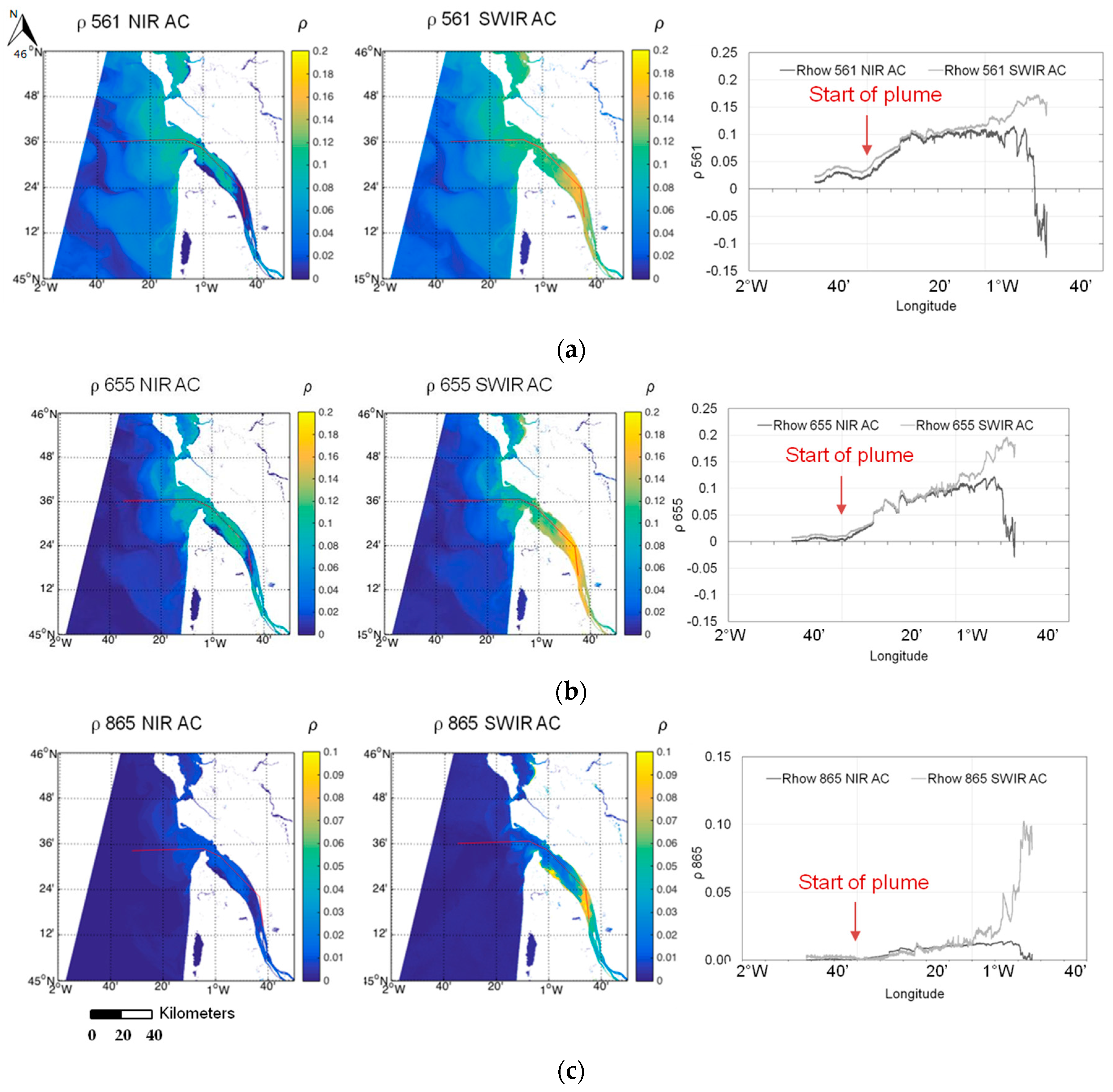
Figure 5 shows the water reflectance values in the OLI green, red and NIR bands obtained applying the ACOLITE-NIR (left column) and ACOLITE-SWIR (right column) atmospheric corrections. The SWIR AC results in water reflectance values at 561 nm 3% (NRMSE) higher than the values obtained applying the NIR AC over the clearest waters (where ρ 561 < 0.001 and ρ 655 < 0.005, as defined by Vanhellemont and Ruddick, 2015) of the transect compared. In the 655 nm band, the difference between the values obtained with the two methods is below a 5% difference for ρ 655 < 0.1. At higher ρ 655 values, found in the Gironde Estuary where the water is more turbid, the NIR AC fails and provides near-zero and even negative values. The spatial variability was calculated for offshore waters (ρ 655 < 0.005), estimating the NRMSE (%) of several 8 × 8 pixel boxes, resulting in an average variability of 5% for the SWIR AC, which could be interpreted as noise. Hence, the mean difference between the NIR AC and SWIR AC for all the bands (areas with low levels of water turbidity in low-turbidity offshore waters) was calculated and proved to be lower than the calculated computed spatial variability. As the NIR AC fails for higher water reflectance (ρ 561 > 0.1, ρ 655 > 0.1, ρ 865 > 0.02), the SWIR AC is the most appropriate correction for the selected study areas. These comparisons are conducted for the transect shown in Figure 5. These results are in accordance with those obtained by [19], who were the first to show the capabilities of Landsat 8/OLI and the SWIR AC to derive accurate ρ values in turbid coastal waters.

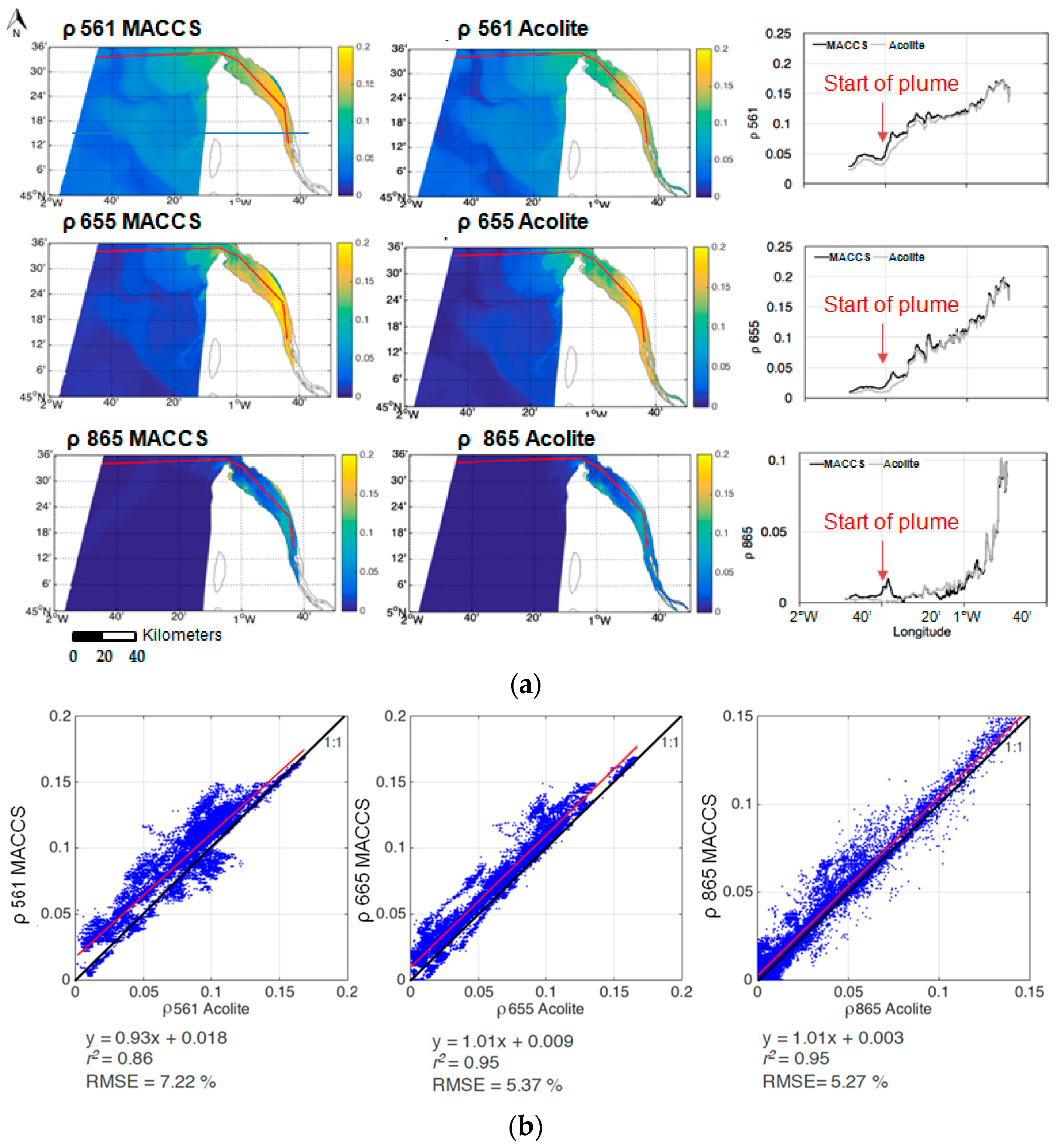
3.1.1. ACOLITE vs. MACCS Products Comparison

Here, the ACOLITE SWIR AC and Theia Data Center MACCS water reflectance products are compared (Figure 6). The highest differences were observed over the less turbid waters, but in general a good agreement exists between both products. The flagged (grey) pixels on MACCS maps over the estuary correspond to the limit of the tile provided by the MACCS-Theia Land Data Center (longitude > 0°45′W). Figure 6b compares ρ values in the green, red and NIR bands obtained by applying both atmospheric corrections to the selected images (Table 5). The selected images were acquired at different periods of the year and for different tidal conditions. The best correlations were obtained for the red and the NIR bands with coefficients of determination of 0.95, a slope close to 1 and a NRMSE around 5%. The maximum differences were observed in the green band (NRMSE = ~7%).

The MACCS algorithm is based on land pixels and estimates the aerosol optical thickness combining a multi-spectral assumption, linking the surface reflectance in the red and blue wavebands, and the assumption that multi-temporal observations of a given area should yield similar surface reflectance when separated by a few days. However, this method is not able to estimate the aerosol model and uses a constant model for a given site, which is a disadvantage for regions where the aerosol model is subject to large spatial variations, such as coastal regions. Instead, the ACOLITE AC method estimates the aerosol type using SWIR bands in clear water pixels for each image. In this study, the aerosol type was assumed to be constant over a single OLI tile (170 × 185 km²), but there is an option provided by the ACOLITE software to allow the type to vary spatially. Research [19] demonstrated that products from OLI compare well with those of MODIS Aqua and Terra, using the SWIR bands corrected atmospherically with ACOLITE. For this reason, and since the ACOLITE AC uses an ocean color approach, this method is considered more appropriate for the coastal waters of the study regions, even though the MACCS method is proved to provide satisfactory results over the most turbid waters. Another reason explaining the differences between both atmospheric corrections is that the MACCS AC applies a continental model in this area, while it has been demonstrated that the maritime model is dominant in the Gironde area [58]. The aerosols of maritime origin are almost non-absorbent, so an overestimation of aerosol absorbance is expected when applying a continental model, especially in offshore waters where there is no land aerosol influence. The reason for the green band differences observed is unclear; it could be due to an overestimation caused by the MACCS AC, or an underestimation by the ACOLITE AC caused by a green band overcorrection. However, as the major differences are observed for the lower ρ_w values (Figure 6b), this dissimilarity is probably related to a flawed correction over offshore waters, where low green ρ_w values are usually found. Studies found on the use of the MACCS AC over coastal areas did not provide information that could explain the differences observed [42,58] other than those already mentioned. Since the green band NRMSE percentage remained low enough (<7%) for the purpose of this study, a deeper analysis on the reasons for these differences was considered out of scope.

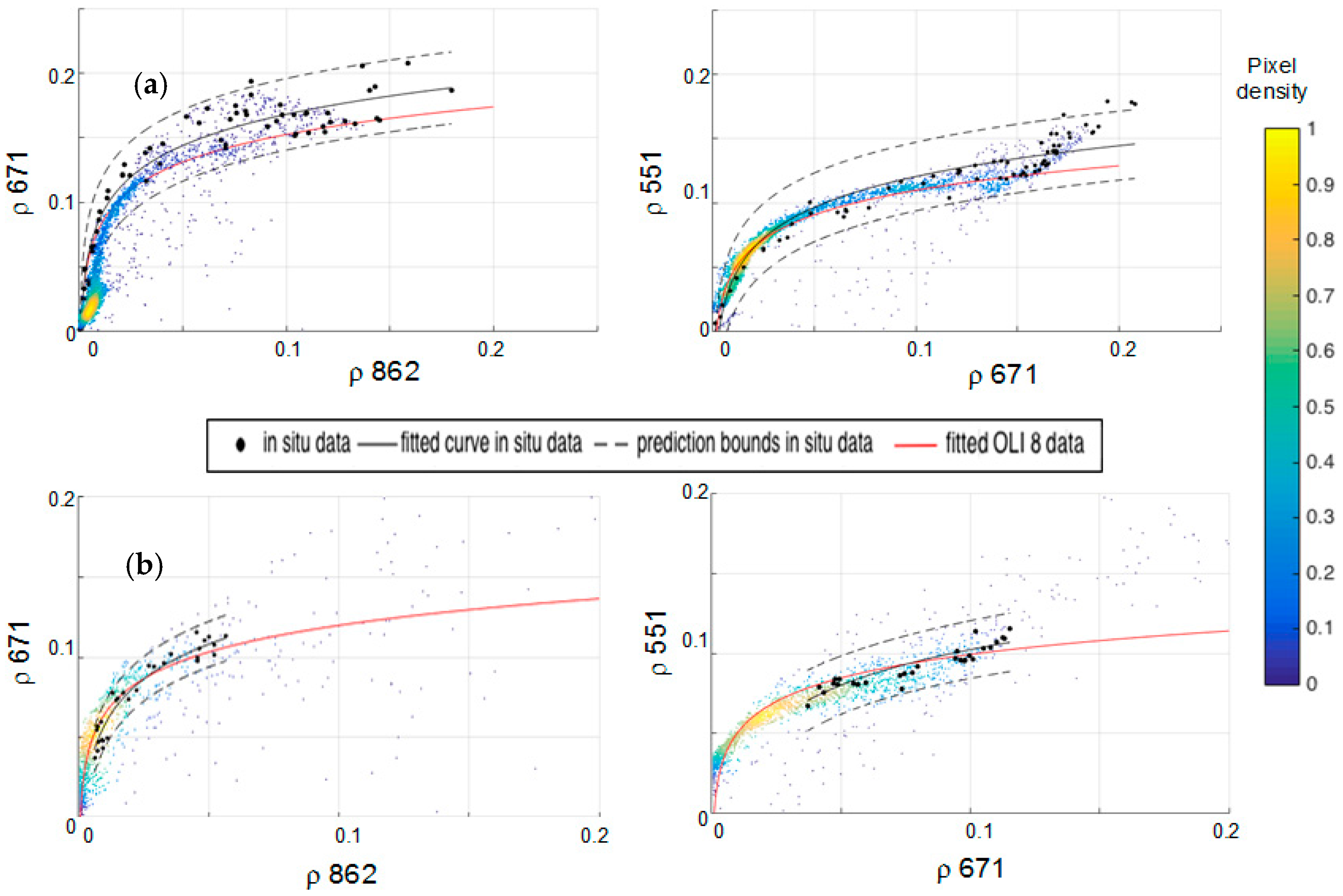
3.1.2. Validation of Atmospheric Correction

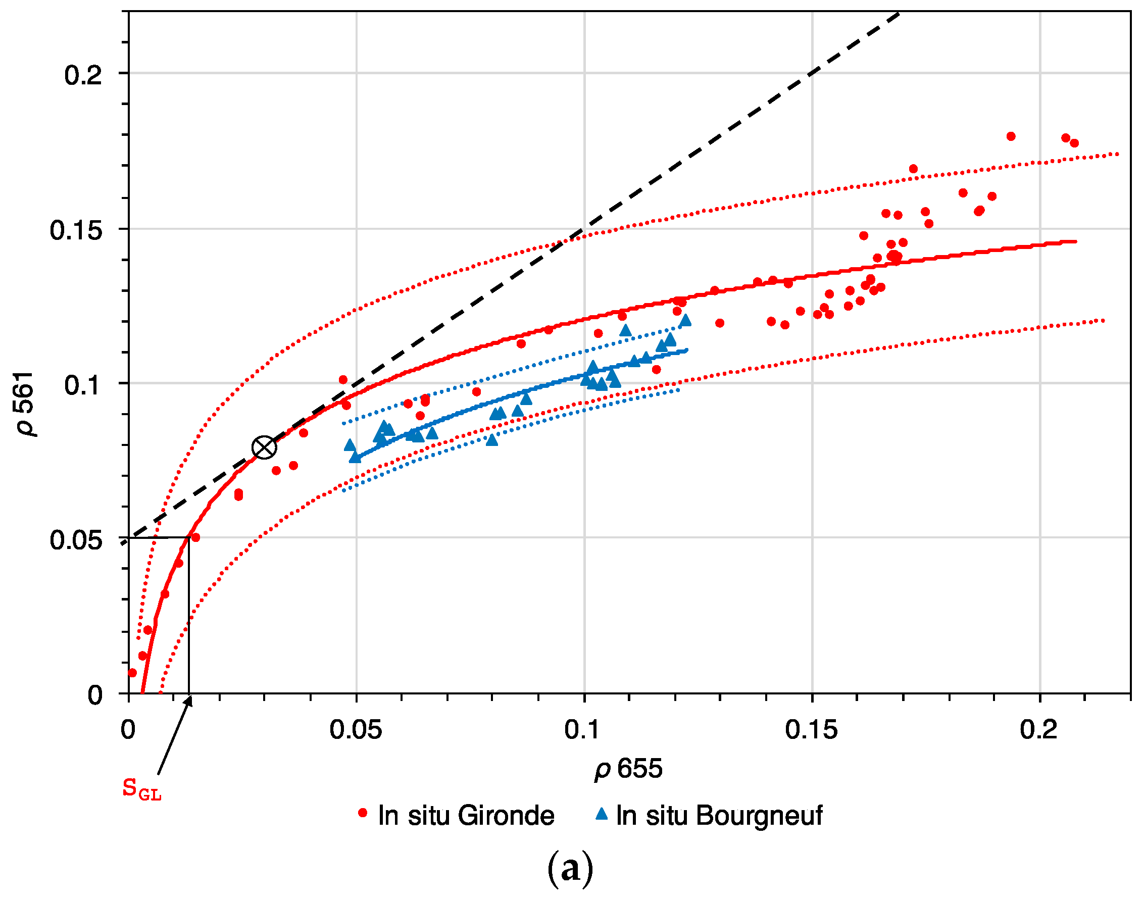
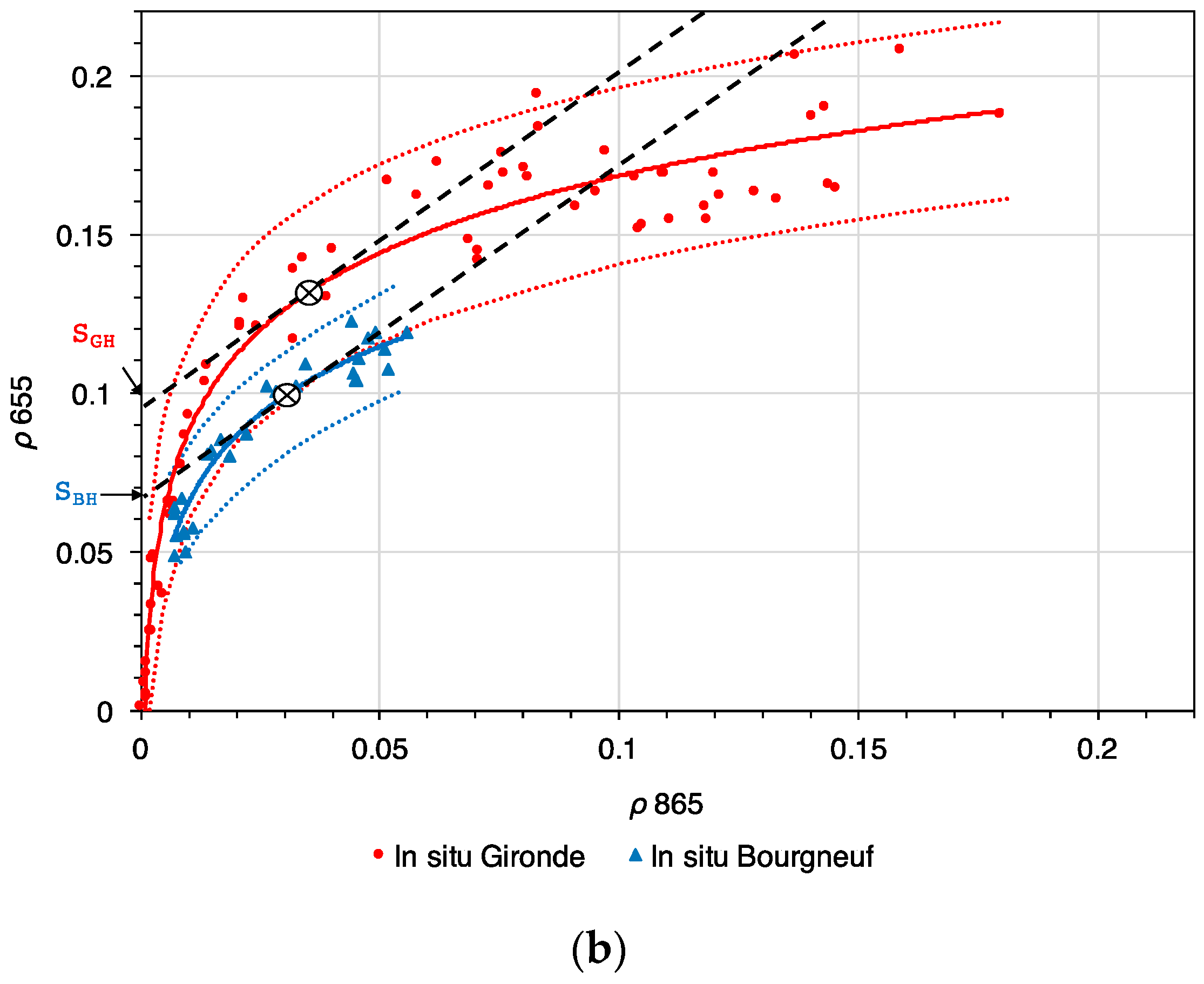
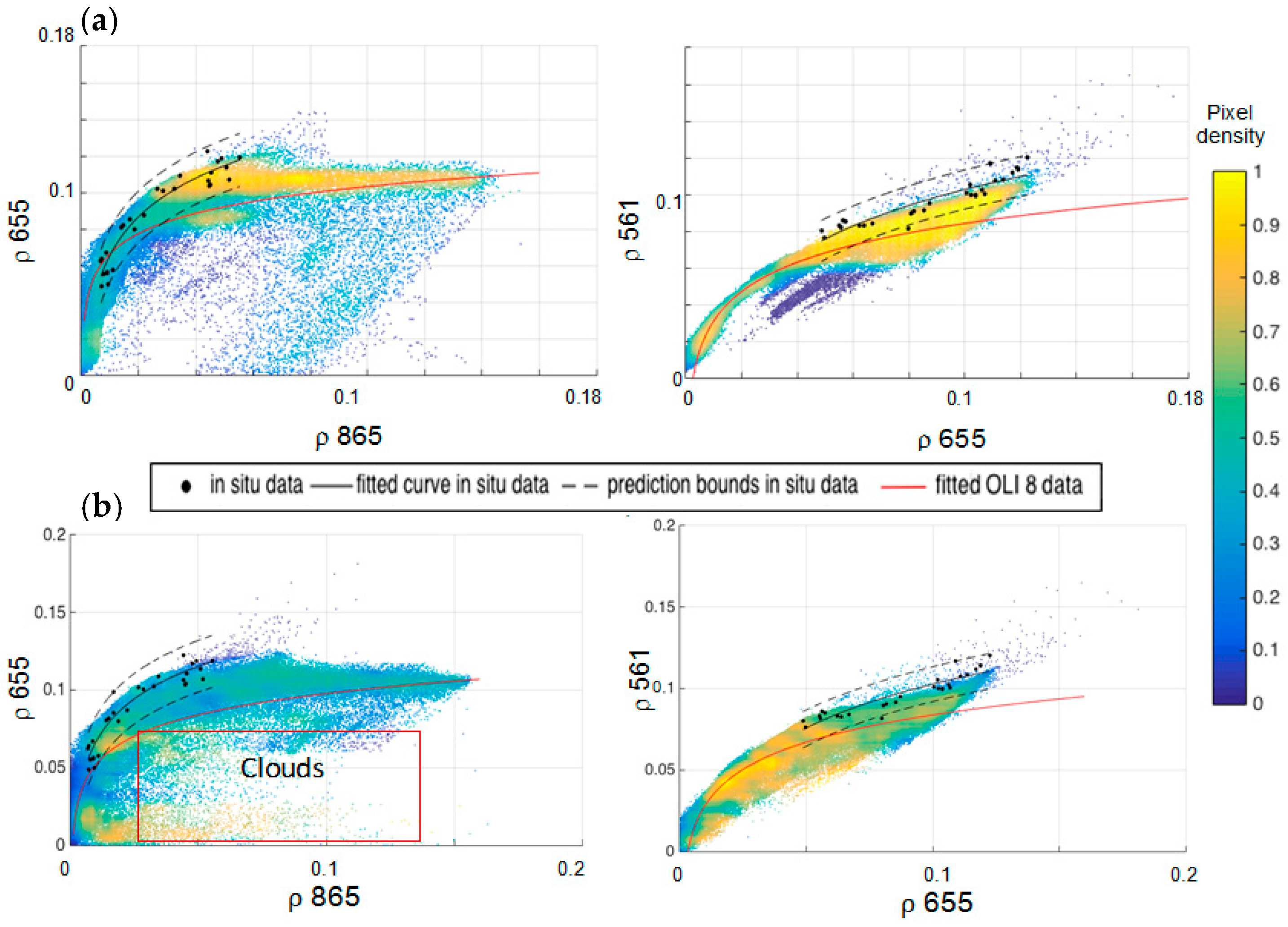
Figure 7a shows the band-to-band ρ value scatter-plots derived from four OLI satellite images of the Gironde Estuary (a and b) and for the Bourgneuf-Loire area (c and d). The same band-to-band ρ value scatter-plots derived from in situ measurements are superimposed. In the case of the Gironde area, the in situ values accurately match the OLI-derived reflectance values, and the logarithmic regressions for both datasets follow the same trend. In the case of the Bourgneuf-Loire area, the trend divergence between in situ and satellite datasets is more significant. This is mainly due to the dispersion observed on the satellite dataset caused by the presence of clouds (Figure 7) on the image acquired on 12 April 2013. The ACOLITE software provides a good mask for clouds, but in some cases cloud shadows or cloud edges are insufficiently masked, introducing significant scatter. Nevertheless, there is a fair overlap between in situ and satellite data for this area as well, taking into account the dataset number difference (in situ stations n = 29 vs. satellite pixels n = ~20,000) and the effect of cloud pixels from 12 April 2013. This image was selected because it was acquired on the last day of the field survey carried out in this area, in April 2013.

Similar ρ band-to-band comparisons were conducted between VIIRS-derived images, and in situ–measured water reflectance at bands centered at 551, 671 and 862 nm (Figure 8). A fair match is obtained between field and satellite datasets for both the Gironde and the Bourgneuf-Loire areas. As can be observed, the in situ (black line) and satellite (red line) regression curves overlap. This demonstrates that the atmospheric correction applied to the VIIRS images, using the SWIR bands and the Seadas (version 7.3), is appropriate for this type of environment.

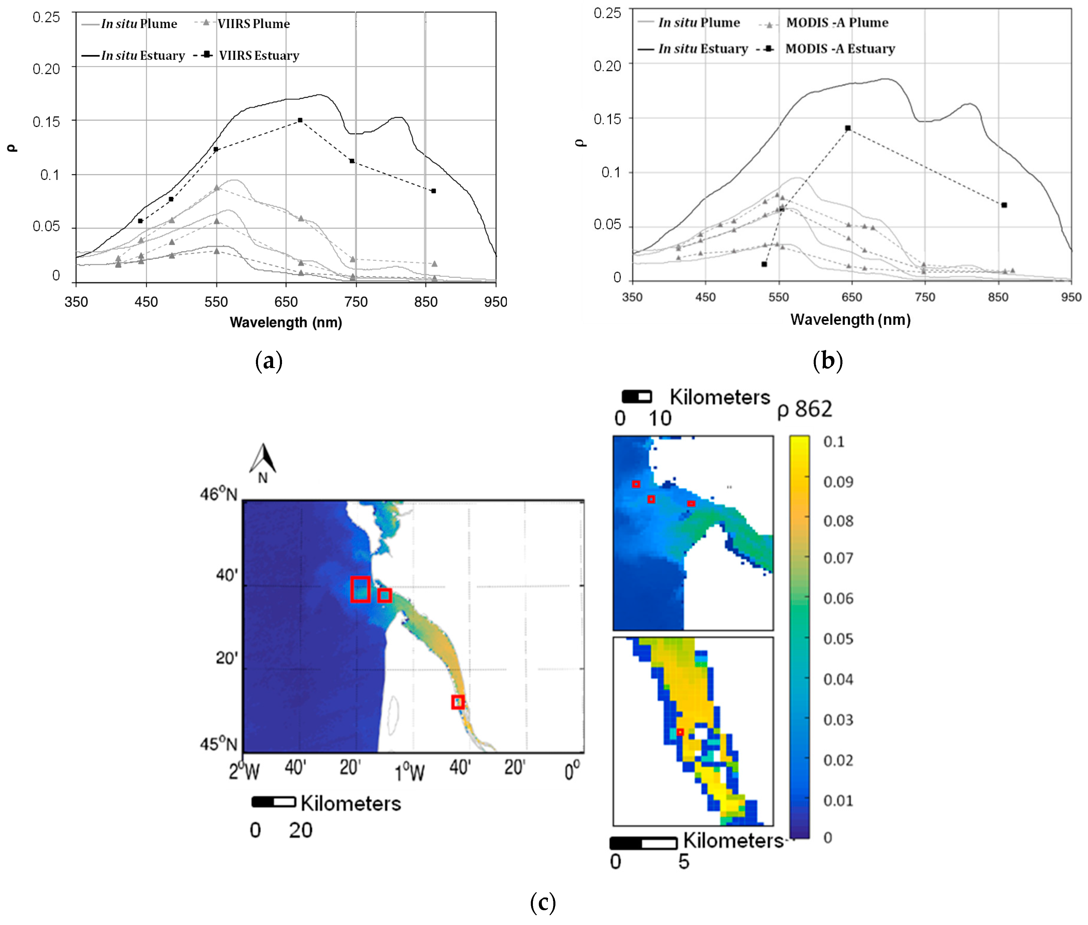
Figure 9 presents a comparison between in situ–measured and satellite-derived reflectance spectra corresponding to VIIRS and MODIS Aqua images acquired on 12 June 2012, 15 July 2014, 16 July 2014. Satellite data were atmospherically corrected using the SWIR option as well. A good match was obtained for the plume area, but in the estuary, the satellite-derived reflectance was systematically lower than values measured in situ at the Pauillac station. This is due to the size sampling differences (satellite vs. in situ) and the effect of the land reflectance in land/water border pixels. Water pixels located near the shore may be contaminated by the land signal, causing erroneous water reflectance estimates. This underestimation in the case of VIIRS (Figure 9a) is lower than in the case of MODIS, where a particularly sudden decrease is observed for the lower wavelengths. This is caused by the use of the MODIS band B5 (1240 nm), which causes an overcorrection in the shorter wavelength band.

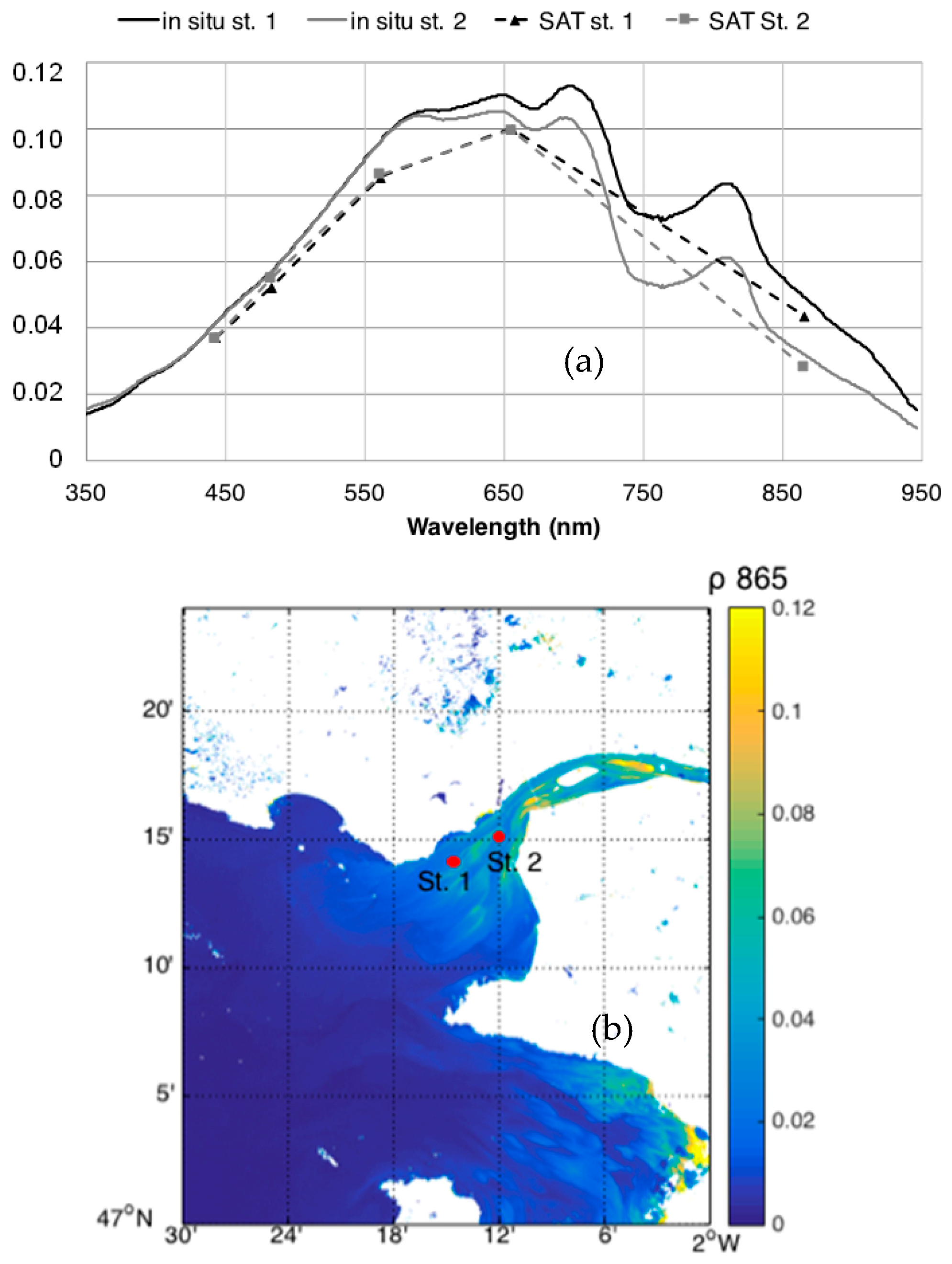
In Figure 10, the reflectance spectra measured in situ on 11 April 2016 at 10:26 (Station 1) and at 11:16 (Station 2) are compared to the OLI-derived values (image acquired at 10:53). There is a closer match between the water reflectance values measured at Station 2 than at Station 1. This could be due to the lower time difference between the image acquisition and the in situ measurement for Station 2 (23 min) than for Station 1 (27 min), together with the significant small-scale variability of the SPM concentration in this specific area given that measurements were conducted during the ebb tide. In general, satellite products appear to underestimate the ‘true’, i.e., field-measured, water reflectance. Valid match-ups with MODIS and VIIRS were not obtained on the same day.

The comparison between in situ and satellite data products resulted in a good match between the green-red and red-NIR bands, with some discrepancies. In general, the trends observed for the satellite data were lower in the higher reflectance values. This is due to the difference in the amount of data (in situ stations n = 29 vs. satellite pixels n = ~20,000) and to cloud shadow and land effects on coastal pixels. Regarding the OLI red-green bands’ (655 vs. 561 nm) comparison, a break was observed between the 0–0.15 and the 0.15–0.2 intervals. If the fit would have been made for values of ρ 655 <0.08, the red and black curves in Figure 7 and Figure 8 would have had a better correspondence for the lower reflectance values, so better results would have been obtained if the comparison was achieved by intervals (e.g., 0–0.08, 0.8–0.2). However, showing the entire data range provides a better understanding of the type of data obtained in situ and from satellite remote sensing measurements, and since the in situ data matches the satellite data, the atmospheric correction was considered to provide realistic reflectance results. The switching bounds were determined using field data, so a better match between the two types of data (in situ vs. satellite) would not affect the switching bound values selected.

Differences observed between in situ and satellite data, in Figure 9 and Figure 10, could be due to several reasons: (1) an overcorrection of the atmospheric contribution in the SWIR method; (2) the spatial difference between the satellite pixel and field measurements (250/750 m² pixel versus ~1 m²); (3) the near-shore location of the station in the estuary. Option 3 appears to be the most plausible, as the pixel selected for the comparison did not correspond exactly to the location of the Pauillac field station: the next pixel away from the shore was selected to avoid the land effect. Thus, the reflectance values at this location are different to the ones measured in situ at Pauillac. In the case of MODIS (Figure 9b), there is an obvious overcorrection inside the estuary, due most probably to the low pixel resolution for this area combined with the selection of the 1240 SWIR band. This effect was also observed in the highly turbid waters of the La Plata river by [52].

3.2. OLI-VIIRS Comparison

Water reflectance values in the green, red and NIR OLI bands (561, 655 and 865 nm) were re-sampled by neighborhood, averaged to a grid of 750 m resolution and then compared to VIIRS-derived values at 551, 671 and 862 nm bands using a common grid. This comparison was achieved for the image acquired on 12 April 2013 (

Table 7. Slope, offset and determination coefficient derived from the comparison of OLI and VIIRS bands from one image acquired on 12 April 2013 (time difference between OLI and VIIRS data acquisition = 3 h).

Bands Region Compared	Slope	Offset	r2
green
Gironde	0.83	0.013	0.71
Bourgneuf-Loire	0.64	0.03	0.67
red
Gironde	0.66	0.017	0.6
Bourgneuf-Loire	0.99	−0.005	0.42
NIR
Gironde	0.29	0.008	0.038
Bourgneuf-Loire	0.87	0.008	0.13

). A fair correspondence was found in the Gironde area for this cloud-free image with a large range of water reflectance values, taking into account the significant overpass time difference between both sensors (~3 h) and the large tidal dynamics occurring in this region, as well as the bandwidth differences between the two satellite sensors. The best correspondence was obtained in the green bands (slope = 0.83, r² = 0.71), followed by the red bands (slope = 0.66, r² = 0.6), and the NIR bands (slope = 0.29, r² = 0.38), even though substantial scatter was present. In the case of the Bourgneuf-Loire area, the best correspondence was obtained between red bands (slope = 0.99, r² = 0.42), followed by the NIR bands with a better slope, but with more scatter (slope = 0.82, r² = 0.1), and the green bands (slope = 0.64, r² = 0.67). Differences between both areas were possibly due firstly to the different optical characteristics and dynamics occurring in both areas, and secondly to a failure of the VIIRS atmospheric correction inside the Gironde Estuary. This exercise was not conducted for MODIS images, because comparisons have already been carried out in similarly turbid waters [19].

Comparisons between OLI and VIIRS products were not found in the literature. However, there is an increasing interest in the exploitation of VIIRS products for coastal studies as this satellite sensor is considered to provide continuity to MODIS. In this study, the VIIRS performance was assessed in highly turbid coastal waters; it showed good results in coastal waters, but the bands’ spatial resolution was too coarse to be used inside the estuary. Nevertheless, the results presented here are promising, as this sensor is still being calibrated, its performance is being tested [59] and methods are currently being developed to use the high-resolution bands in coastal waters [60]. The water reflectance values derived from satellite data were slightly lower than the values measured in situ. This is mainly due to the difference in sampling size, as OLI images have a resolution of 30 m, while the water volume sampled in situ was much lower (~10 L). Research [57] showed good agreement between OLI and in situ spectra in low- to high-turbidity waters. This study confirms their findings in study areas with different SPM characteristics with respect to the North Sea [21].

In summary, the SWIR atmospheric correction appears to be the most appropriate for the selected study areas, including low- to high-turbidity waters (Figure 5a). ACOLITE software corrections provided satisfactory water reflectance values for OLI images, in good agreement with MACCS reflectance products (Figure 6a), as already highlighted in previous studies (e.g., [42]). In relation to VIIRS, there is a good correspondence between in situ and satellite-derived water reflectance for both study areas (Figure 8 and Figure 9, Table 7), although additional in situ–satellite match-ups would be necessary to draw further conclusions. The problem with the atmospheric corrections of MODIS data is the use of the 1240 nm band, which can provide reflectance values above zero in highly turbid waters, causing an overcorrection to the visible bands [52,61].

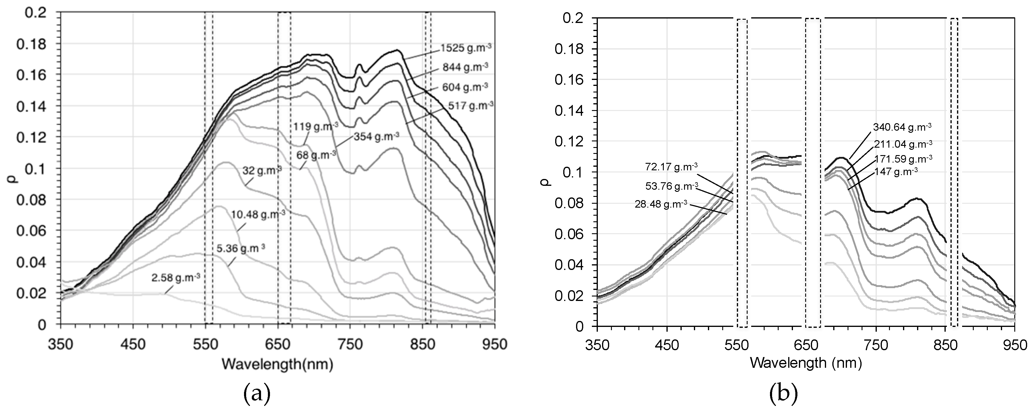
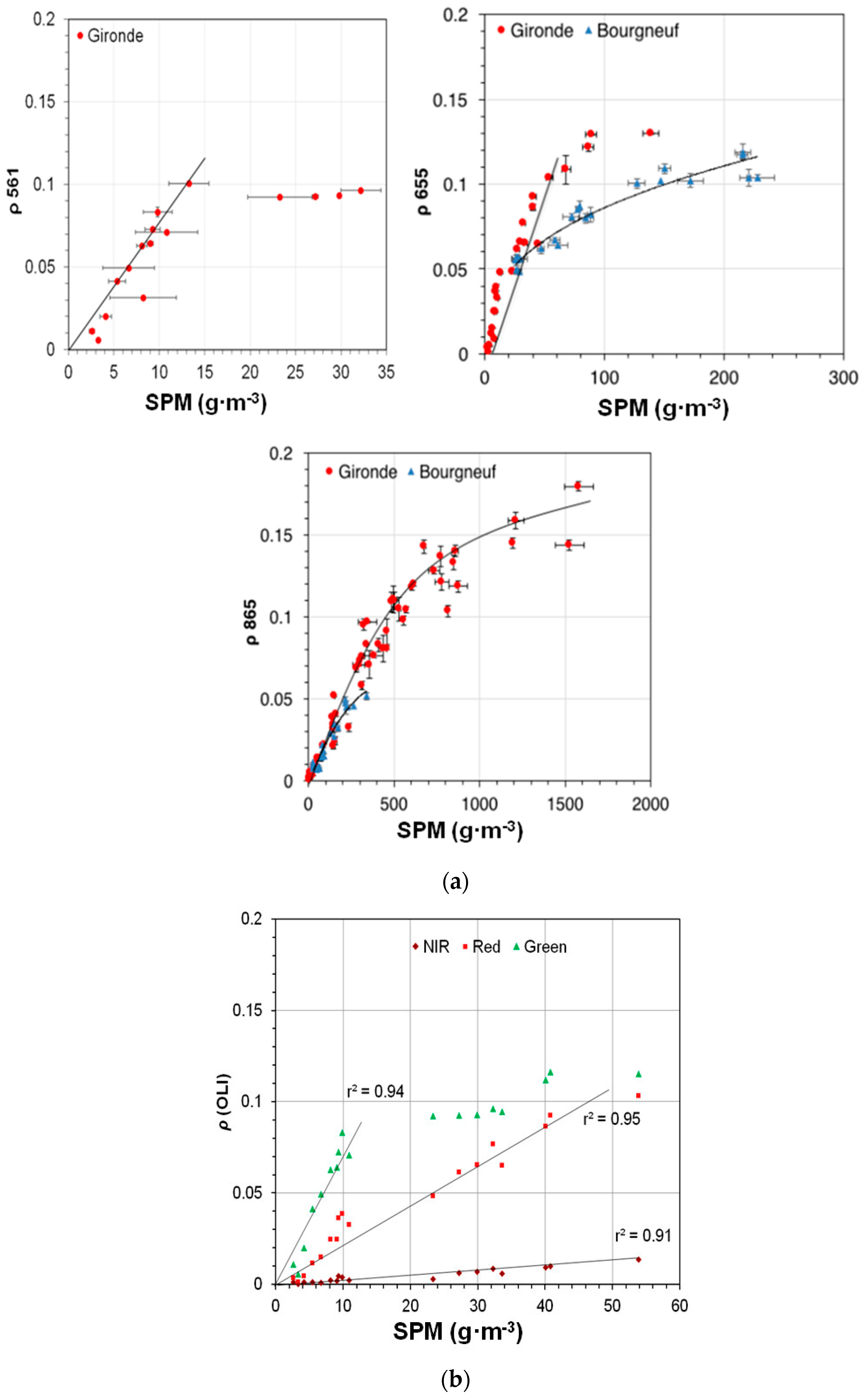
3.3. Multi-Conditional SPM Algorithm

Figure 11 presents the application of the switching SPM model (Table 2) combined with the smoothing procedure (Equations (3)–(6), Table 3) to the OLI image of the Gironde Estuary, acquired on 2 February 2015. The transect along the plume and estuarine area proves that the developed switching and smoothing methods allow a smooth transition between the SPM concentration remotely sensed from the offshore low-turbidity waters to the highly turbid waters inside the estuary. Note that the SPM NIR band values are highly noisy for concentrations lower than 50 g·m⁻³.

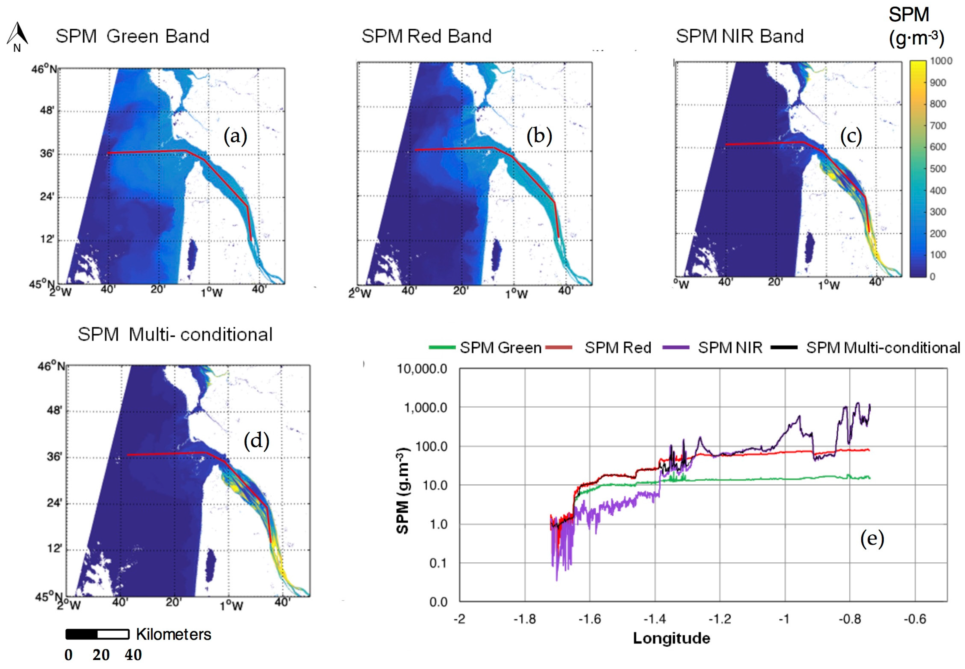
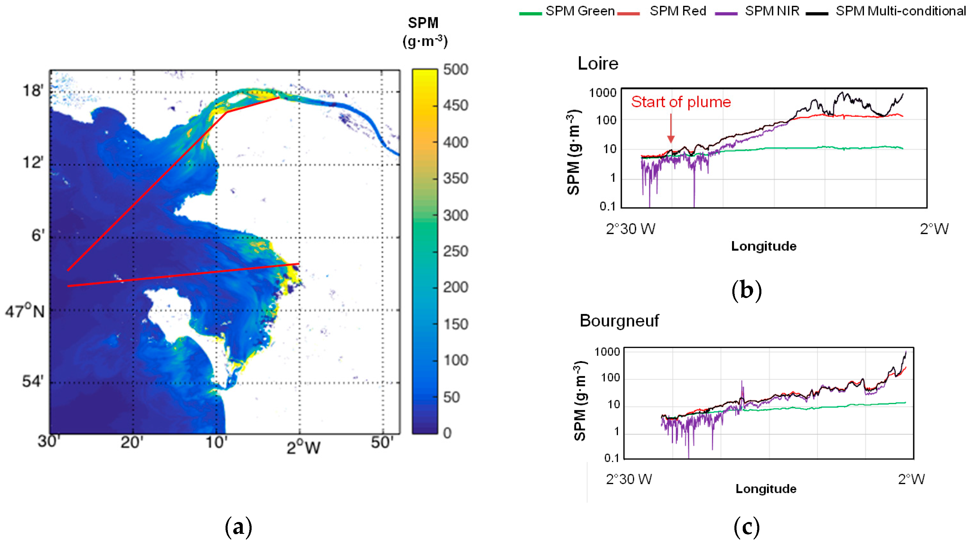
Figure 12 shows the application of the SPM multi-conditional algorithm to a cloud-free image acquired on 12 April 2016 over the Bourgneuf-Loire area using the procedure presented in Section 2. The smooth transition between the remotely sensed SPM concentration is clearly observed along both the Loire and Bourgneuf transects. As shown in Figure 12b,c, the SPM multi-conditional algorithm (black line) starts estimating SPM using the green band equation in the clear water area (green line) for both the Loire and Bourgneuf transects. Then, as the SPM concentration increases, due to the river plume in the Loire transect and to the mudflat SPM re-suspension in the Bourgneuf area, the multi-conditional algorithm switches to the red band–estimated SPM (red line). Then, as the red band reflectance increases due to the near-shore SPM concentration increase, the algorithm switches to the SPM calculated with the NIR band equation. The figure clearly shows a high variability in SPM estimation using the NIR band equation (purple line) in clear waters (2°30′W–2°20′W), proving the importance of using equations appropriate for each concentration SPM range.

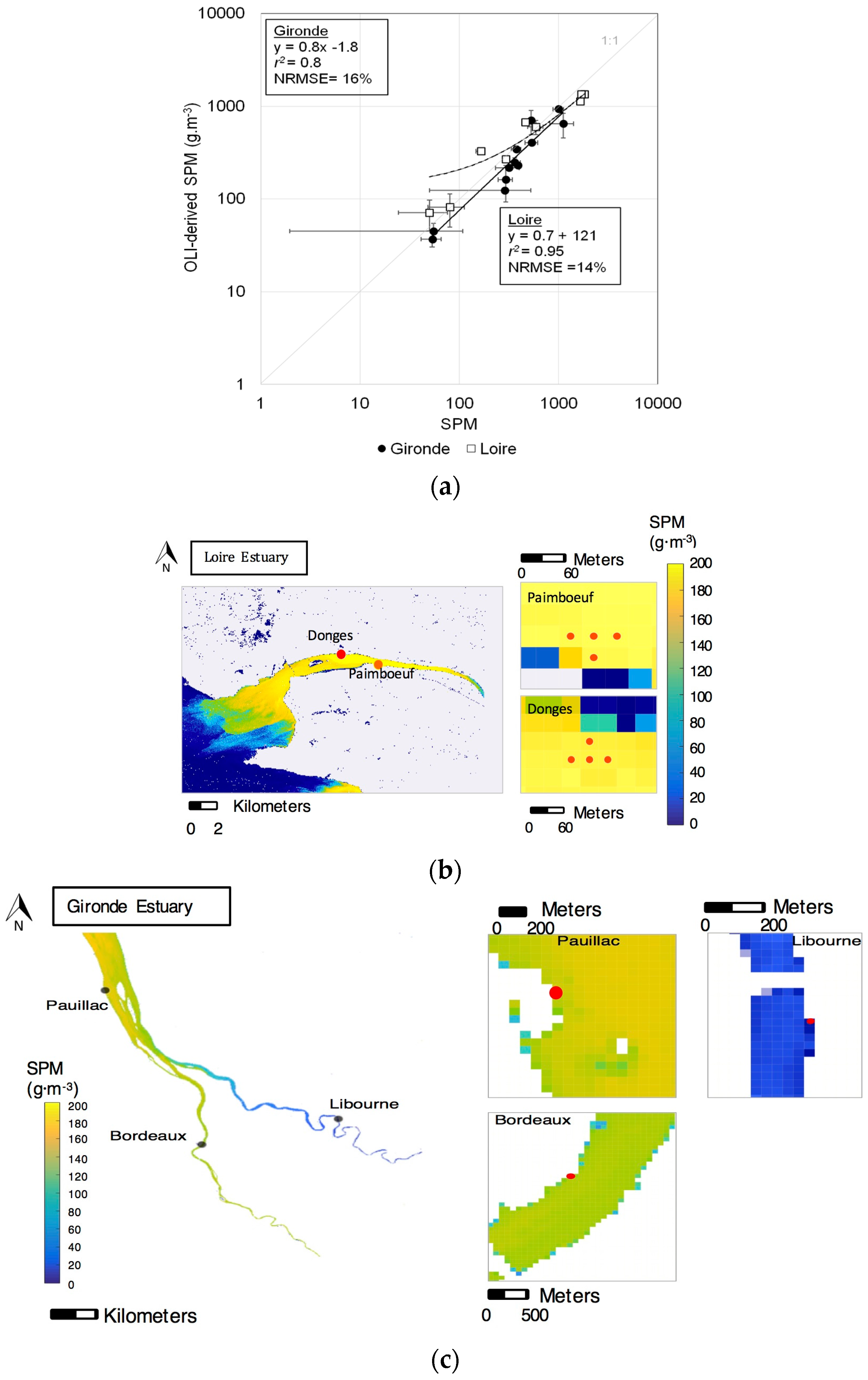
Match-ups between in situ–measured SPM (MAGEST and SYVEL network stations) and OLI-derived SPM concentrations were then analyzed (Figure 13,

Table 8. Slope, adjusted r², percent NRMSE (%) and offset resulting from the match-ups between in situ measurements from the MAGEST (Gironde) and SYVEL (Loire) network stations and the OLI-derived SPM concentration obtained using the different empirical and semi-empirical models shown in Table 2 and Table A2 (appendix).

	Exponential 1 Band	Exponential Ratio	Polynomial 1 Band	Polynomial Ratio	Nechad et al. (2010) [16] NIR	Doxaran et al. (2009) [18]	Gernez et al. (2015) [42]	SPM Multi-Conditional
Gironde
Slope	0.65	1.1	0.8	1.1	0.9	1.4	0.6	0.8
r2	0.8	0.7	0.8	0.74	0.76	0.6	0.6	0.8
NRMSE (%)	20	22.3	16.4	19.8	17	36.5	44.7	16
offset	66	16	−3	33	−19	−185	−24	−1.8
Loire
Slope	0.66	0.9	3.53	0.3	0.67	0.3	0.2	0.67
r2	0.72	0.4	0.76	0.5	0.95	0.4	0.5	0.95
NRMSE (%)	29.7	48	158	40	14	39	46.8	14
offset		58	−3	75	−19	46.3	56	121

) to prove that the multi-conditional algorithm provides accurate SPM concentrations. The dates to the OLI images used for satellite—in situ match-ups are shown in Table 6, together with tidal ranges and tide times (low and high tides) in the Gironde Estuary (Pauillac) and Loire Estuary (Donges) at those dates. The in situ SPM concentrations for the Gironde Estuary were derived from the turbidity measurements (in FNU) at the stations and the turbidity-SPM relationship was established with in situ measurements taken in the Gironde Estuary. In general, OLI provided good SPM estimates at the Pauillac and Libourne stations (r² = 0.8 and 0.95, NMRSE = 16% and 14%, respectively, for Gironde and Loire). Previous match-ups using the MAGEST network measurements and SPOT 5 satellite data provided good results with higher pixel resolutions than OLI, showing the capacity of these stations for satellite imagery validation [42]. Additionally, the SPM concentration calculated using different models (refer to Table A2 in the appendix), including the models of [18,42], were matched to in situ SPM measurements. The resulting match-ups (Table 8) show that the multi-conditional algorithm provided, for both the Gironde and the Loire areas, the best of fit (r² = 0.8, 0.67) and low error (16%, 14%) combination when compared to SPM estimated using other models. The combination of several models adapted to each concentration range is the main reason for this result, together with the selection of the best-fitted models. As proved by other studies [35,36,37], the selection of a specific model combining different bands is an improvement when estimating the SPM concentration in coastal waters.

Table 8 shows the in situ-satellite match-up results using different SPM models. In the case of the Gironde area, the fit, slope, NRMSE (%) and offset when using the band-ratio and single-band exponential and polynomial regressions were similar. Slightly better results were obtained with the exponential NIR-red band ratio models (r² = 0.7, slope = 1.1, NRMSE = 22.3%, offset = 16) compared to the exponential NIR band model (r² = 0.8, slope = 0.65, NRMSE = 20%, offset = 66), but the polynomial single-band model performed better when using the single NIR band (r² = 0.8, slope = 0.8, NRMSE = 16.4%, offset = −3), compared to the band ratio (r² = 0.74, slope = 0.9, NRMSE = 19.8%, offset = 33). The SPM concentration estimates did not improve when using equations published in other studies for the same study areas [18,42] providing larger NMRSEs (36.5%, 44.7%) and offsets (−185, −24), compared to the results obtained with the multi-conditional algorithm (slope = 0.8, r² = 0.8, NRMSE = 16%, offset = −1.8). In the case of the Bourgneuf-Loire area, the combination of the re-calibrated NIR and red band semi-empirical models from Reference [16] with the multi-conditional algorithm provided the best fit and lowest error (slope = 0.67, r² = 0.95, NRMSE = 14%, offset = 121). In this case, the performance of the algorithm will improve with a re-calibration of the models with additional in situ data.

The configuration of the pixels selected for the match-ups is shown in Figure 13. OLI-derived SPM estimates provided good match-up results with the in situ measurements. In the case of the Bourgneuf-Loire area, instead of using one pixel for the match-ups, as in the case of Gironde, an average of four pixels was used, as it provided the best results. Vertical error bars show the standard deviation of the four pixels selected, in the case of the Loire area (see Figure 13b), and of the three nearby pixels in the case of the Gironde area (shown as red rectangles), even if a single pixel was used for the match-ups (red circle) in Figure 13c. Horizontal error bars correspond to the temporal SPM variability ±10 min from the satellite overpass time. There appears to be an underestimation by the algorithm at SPM concentrations above 100 g·m⁻³ and a slight overestimation below 500 g·m⁻³ (and above 100 g·m⁻³) in the Bourgneuf-Loire area, while the Gironde algorithm seems to overestimate values above 500 g·m⁻³. This tendency was also observed by [42] using SPOT 4 data, where the same pixel configuration was used for the Loire match-ups. The imprecision observed for these match-ups is due to several factors, such as the accuracy of the SPM algorithms, the errors and uncertainties in field measurements, the spatial differences between the sampling station and satellite pixel location, as well as uncertainties related to atmospheric corrections. Different SPM models including band ratios, such as those developed by [18,42] for these areas, were applied to the images, but the match-up results did not improve (see Table 8).

Figure 14 compares the SPM concentrations derived from OLI, VIIRS and MODIS (Aqua) satellite data recorded on the same day over the Gironde Estuary. Water reflectances at 655 (OLI), 671 (VIIRS), 645 nm (MODIS aqua) show a similar trend along the transect. VIIRS products provided higher values than OLI in general, up to the most upstream section of the Estuary, where there was a sharp decrease. It corresponded to a failure of the atmospheric correction, due to the low VIIRS spatial resolution for this particular area. This failure was also observed along the MODIS transect, where the most upstream pixels are missing, resulting in a sudden SPM concentration decrease. Generally, the MODIS and OLI transects overlap up to the most upstream section of the estuary, where SPM concentrations are overestimated by MODIS. This is due to the proximity of the land on the last transect pixels, which, as seen in Figure 13d, results in a rapid decrease of the SPM concentration. In this particular region, the reflectance at 859 nm showed a fast increase for MODIS, which was not observed in the OLI 865 band. Hence, particular attention needs to be paid to the near-shore pixels, where the atmospheric correction may provide inaccurate water reflectance estimates, resulting in inaccurate SPM retrievals. For practical reasons, the same switching bounds applied to OLI were used for VIIRS and MODIS Aqua. However, the fine adjustment of the switching bounds to each sensor’s spectral bands could provide better results. Despite the fact that the MODIS atmospheric corrections provided underestimated water reflectance values, the transect comparison showed a good match between the three SPM maps.

Overall, the multi-conditional SPM algorithm provides a smooth transition between SPM models for three different sensors over an area that goes from low- to high-turbidity surface waters. The band-switching technique allows keeping the optimal sensitivity of ρ to SPM variations and avoiding the saturation of ρ in (highly) turbid waters. The study areas were characterized by a high amount of cloudy days, and taking into account that OLI images are only available every 16 days, it was difficult to obtain numerous cloud-free images to apply the SPM algorithm. Again, the purpose of this study was not to provide the best SPM models for each area, but to develop a method and test it on selected satellite data recorded for optimal conditions (cloud-free, clear atmosphere) representative of a wide range of SPM concentrations in coastal and estuarine waters. Similar methods have already been developed [35,36], but the procedure presented in the present study (1) automatically selects the model switching bounds based on in situ measurements; (2) fully applies the method to real satellite data provided by three different sensors; and (3) validates the results based on match-ups with field data.

4. Conclusions and Perspectives

In this study we have shown that satellite imagery from MODIS, VIIRS and OLI satellites can be used to reliably estimate SPM in coastal waters over a very wide concentration range (1–2000 g·m⁻³) using a novel multi-conditional algorithm. In situ SPM and water reflectance measurements were used to calibrate switching SPM algorithms based on multiple SPM vs. ρ relationships. For each specific SPM range (<10, 10–50, and >50 g·m⁻³), the ρ in specific spectral bands (green, red and NIR, respectively) was found to be more sensitive to changes in the SPM concentration, and the corresponding best-fitted SPM vs. ρ relationship was selected. These relationships were established empirically and semi-empirically and calibrated for clear to highly turbid waters in two study site areas: the Gironde and the Bourgneuf-Loire area estuaries. The selected models for each SPM range and each band were chosen based on goodness-of-fit tests (r²) and NRMSE (%) results from the validation exercises. In the case of the Gironde estuary, the best-performing models were a single-band, second-order polynomial relationship for the NIR band (r² = 0.97; NRMSE = 9.11%) and a linear relationship for the red (r² = 0.81; NRMSE = 7.23%) and green bands (r² = 0.81; NRMSE = 16.41%). In the case of the Bourgneuf-Loire area, the best-performing model was the semi-empirical relationship published by [16], re-calibrated with the in situ dataset, for both the NIR (r² = 0.93, NRMSE = 7.81%) and red bands (r² = 0.82, NRMSE = 18.22%).

The bounds for switching between models were based on water reflectance values derived from the saturation points of the most sensitive bands. The bounds were selected by means of band comparisons from field water reflectance measurements: ρ (green) vs. ρ (red) and ρ (red) vs. ρ (NIR). The field data points were modeled using a logarithmic regression curve. The actual value of the saturation point, which is also the switching point, was computed as the point where the first derivative of that regression curve (i.e., the slope or tangent) equals 1, as this is the middle point between a completely horizontal (complete saturation) and a completely vertical line. The switching points selected were based on the red band water reflectance values, being the middle band between the green and the NIR. Then, the models were weighted to ensure a smooth transition between different SPM concentrations. The smoothing bounds were derived from the 95% confidence levels of the regression curve following the same procedure as for the switching value calculation. The switching values for each system are reported in Table 3.

To obtain accurate satellite-derived SPM maps, appropriate atmospheric corrections are required in coastal waters. Several atmospheric correction algorithms were compared, and match-ups between satellite and field measurements showed that SWIR-based atmospheric correction algorithms performed best. Alternative approaches such as the MACCS method initially developed for land applications also provide satisfactory results. Despite some inaccuracies in water reflectance retrieval, the SPM concentration can be reliably estimated using the three sensors (MODIS, VIIRS and OLI) in low (SPM ~ 1 g·m⁻³) to highly turbid waters (SPM > 2000 g·m⁻³). However, VIIRS and MODIS images fail inside narrow estuaries (here the Gironde) due to low spatial resolution.

The multi-conditional algorithm presented in this study successfully provided a smooth transition between different SPM models, and was then successfully applied to multi-sensor satellite data. It was proved to provide a smooth transition between different SPM models. Results clearly highlighted the need for switching the SPM algorithm in coastal and estuarine waters where (i) the water reflectance in the green and then red spectral regions rapidly saturated with the increasing SPM concentration, while (ii) water reflectance in the NIR is associated with a low signal-to-noise ratio and significantly underestimates the SPM concentration in clear to moderately turbid waters (Figure 9 and Figure 10). A comparison with in situ data showed that the reflectance measurements undertaken in the field corresponded satisfactorily with the satellite-derived water reflectance (Figure 9), except for the MODIS products inside the estuary. Moreover, the match-up exercise using the SYVEL (r² = 0.95, NRMSE = 14%, slope = 0.7) and MAGEST (r² = 0.8, NRMSE = 16%, slope = 0.8) autonomous stations provided satisfactory results, proving that the selection of the algorithms was appropriate. Still, additional in situ measurements in these areas would improve the calibration of the models and provide better validation results.

The switching bound selection method presented here can be easily applied to any turbid coastal water area associated with wide turbidity ranges, without the need for in situ measurements. The bounds can be directly selected by comparing the water reflectance in the green, red and NIR wavebands directly derived from satellite data to detect the saturation points and infer the switching values (Figure 7 and Figure 8). This study offers the appropriate methodology to study long-term dynamics and trends using satellite imagery in turbid coastal waters. When applied to multi-sensor satellite data, it can significantly contribute to the understanding of the impact of anthropogenic pressures on coastal environments, monitoring water quality, gaining knowledge of estuarine processes and even studying the impact of recent climate change. The multi-sensor approach presented here can be appropriately applied to the latest generation of ocean color sensors (namely Sentinel2/MSI and Sentinel3/OLCI) to study SPM dynamics in the coastal ocean at higher spatial and temporal resolutions.

References

1. Tassan, S. Local algorithm using SeaWiFS data for retrieval of phytoplankton pigments, suspneded sediment and yellow substance in coastal waters. Appl. Opt. 1994, 33, 2369–2378. [Google Scholar] [CrossRef] [PubMed]
2. Warrick, J.A.; Mertes, L.A.K.; Washburn, L.; Siegel, D.A. Dispersal forcing of southern California river plumes, based on field and remote sensing observations. Geo-Mar. Lett. 2004, 24, 46–52. [Google Scholar] [CrossRef]
3. Miller, R.L.; del Castillo, C.E.; McKee, B.A. Remote Sensing of Coastal Aquatic Environments. Technologies, Techniques and Applications; Springer: New York, NY, USA, 2005. [Google Scholar]
4. Doxaran, D.; Froidefond, J.; Castaing, P.; Babin, M. Estuarine, Coastal and Shelf Science. Science 2009, 81, 321–332. [Google Scholar]
5. Doxaran, D.; Leymarie, E.; Nechad, B.; Ruddick, K.G.; Dogliotti, A.I.; Knaeps, E. An improved correction method for field measurements of particulate light backscattering in turbid waters State of the Art. Opt. Express 2013, 24, 3615–3637. [Google Scholar] [CrossRef] [PubMed]
6. Petus, C.; Chust, G.; Gohin, F.; Doxaran, D.; Froidefond, J.-M.; Sagarminaga, Y. Estimating turbidity and total suspended matter in the Adour River plume (South Bay of Biscay) using MODIS 250-m imagery. Cont. Shelf Res. 2010, 30, 379–392. [Google Scholar] [CrossRef]
7. Lorthiois, T.; Doxaran, D.; Chami, M. Daily and seasonal dynamics of suspended particles in the Rhône River plume based on remote sensing and field optical measurements. Geo-Mar. Lett. 2012, 32, 89–101. [Google Scholar] [CrossRef]
8. Vanhellemont, Q.; Neukermans, G.; Ruddick, K. Synergy between polar-orbiting and geostationary sensors: Remote sensing of the ocean at high spatial and high temporal resolution. Remote Sens. Environ. 2013, 146, 49–62. [Google Scholar] [CrossRef]
9. Eom, J.; Choi, J.-K.; Won, J.-S.; Ryu, J.-H.; Doxaran, D.; Ruddick, K.; Lee, S. Spatiotemporal Variation in Suspended Sediment Concentrations and Related Factors of Coastal Waters Based on Multispatial Satellite Data in Gyeonggi Bay, Korea. J. Coast. Res. 2016, in press. [Google Scholar] [CrossRef]
10. Hudson, A.S.; Talke, S.A.; Jay, D.A. Using Satellite Observations to Characterize the Response of Estuarine Turbidity Maxima to External Forcing. Estuaries Coasts 2016. [Google Scholar] [CrossRef]
11. Kubryakov, A.; Stanichny, S.; and Zatsepin, A. River plume dynamics in the Kara Sea from altimetry-based lagrangian model, satellite salinity and chlorophyll data. Remote Sens. Environ. 2016, 176, 177–187. [Google Scholar] [CrossRef]
12. Restrepo, J.D.; Park, E.; Aquino, S.; and Latrubesse, E.M. Coral reefs chronically exposed to river sediment plumes in the southwestern Caribbean: Rosario Islands, Colombia. Sci. Total Environ. 2016, 553, 316–329. [Google Scholar] [CrossRef] [PubMed]
13. Ody, A.; Doxaran, D.; Vanhellemont, Q.; Nechad, B.; Novoa, S.; Many, G.; Bourrin, F.; Verney, R.; Pairaud, I.; Gentili, B. Potential of high spatial and temporal ocean color satellite data to study the dynamics of suspended particles in a micro-tidal river plume. Remote Sens. 2016, 8, 245. [Google Scholar] [CrossRef] [Green Version]
14. Tan, J.; Cherkauer, K.A.; Chaubey, I.; Troy, C.D.; Essig, R. Water quality estimation of River plumes in Southern Lake Michigan using Hyperion. J. Gt. Lakes Res. 2016, 42, 524–535. [Google Scholar] [CrossRef]
15. Doxaran, D.; Castaing, P.; Lavender, S.J.; Castaign, P.; Lavender, S.J. Monitoring the maximum turbidity zone and detecting finescale turbidity features in the Gironde estuary using high spatial resolution satellite sensor (SPOT HRV, Landsat ETM) data. Int. J. Remote Sens. 2006, 27, 2303–2321. [Google Scholar] [CrossRef]
16. Nechad, B.; Ruddick, K.G.; Park, Y. Calibration and validation of a generic multisensor algorithm for mapping of total suspended matter in turbid waters. Remote Sens. Environ. 2010, 114, 854–866. [Google Scholar] [CrossRef]
17. Forget, P.; Ouillon, S. Surface suspended matter off the Rhone river mouth from visible satellite imagery. Oceanol. Acta 1998, 21, 739–749. [Google Scholar] [CrossRef]
18. Doxaran, D.; Froidefond, J.; Castaing, P.; Babin, M. Dynamics of the turbidity maximum zone in a macrotidal estuary ( the Gironde, France ): Observations from field and MODIS satellite data. Estuar. Coast. Shelf Sci. 2009, 81, 321–332. [Google Scholar] [CrossRef]
19. Vanhellemont, Q.; Ruddick, K. Advantages of high quality SWIR bands for ocean colour processing: Examples from Landsat-8. Remote Sens. Environ. 2015, 161, 89–106. [Google Scholar] [CrossRef]
20. Neukermans, G.; Ruddick, K.; Bernard, E.; Ramon, D.; Nechad, B.; Deschamps, P.Y. Mapping total suspended matter from geostationary satellites: A feasibility study with SEVIRI in the Southern North Sea. Opt. Express 2009, 17, 14029–14052. [Google Scholar] [CrossRef] [PubMed]
21. Neukermans, G.; Ruddick, K.G.; Greenwood, N. Diurnal variability of turbidity and light attenuation in the southern North Sea from the SEVIRI geostationary sensor. Remote Sens. Environ. 2012, 124, 564–580. [Google Scholar] [CrossRef]
22. Gordon, H.R.; Wang, M. Retrieval of water-leaving radiance and aerosol optical thickness over the oceans with SeaWiFS: A preliminary algorithm. Appl. Opt. 1994, 33, 443–452. [Google Scholar] [CrossRef] [PubMed]
23. Ruddick, K.G.; Ovidio, F.; Rijkeboer, M. Atmospheric correction of SeaWiFS imagery for turbid coastal and inland waters: Comment. Appl. Opt. 2000, 39, 893–895. [Google Scholar] [CrossRef]
24. Hu, C.; Carder, K.L.; Muller-Karger, F.E. Atmospheric correction of SeaWiFS imagery over turbid coastal waters: A practical method. Remote Sens. Environ. 2000, 74, 195–206. [Google Scholar] [CrossRef]
25. Wang, M.; Shi, W. Estimation of ocean contribution at the MODIS near-infrared wavelengths along the east coast of the U.S.: Two case studies. Geophys. Res. Lett. 2005, 32, L13606. [Google Scholar] [CrossRef]
26. Gohin, F. Annual cycles of chlorophyll-a, non-algal suspended particulate matter, and turbidity observed from space and in-situ in coastal waters. Ocean Sci. 2011, 7, 705–732. [Google Scholar] [CrossRef]
27. Nechad, B.; Alvera-Azcaràte, A.; Ruddick, K.; Greenwood, N. Reconstruction of MODIS total suspended matter time series maps by DINEOF and validation with autonomous platform data. Ocean Dyn. 2011, 61, 1205–1214. [Google Scholar] [CrossRef]
28. Van der Woerd, H.; Pasterkamp, R. Mapping of the North Sea turbid coastal waters using SeaWiFS data. Can. Remote Sens. 2004, 30, 44–53. [Google Scholar] [CrossRef]
29. Doxaran, D.; Froidefond, J.; Lavender, S.; Castaing, P. Spectral signature of highly turbid waters Application with SPOT data to quantify suspended particulate matter concentrations. Remote Sens. Environ. 2002, 81, 149–161. [Google Scholar] [CrossRef]
30. Moore, G.F.; Aiken, J.; Lavender, S.J. The atmospheric correction of water colour and the quantitative retrieval of suspended particulate matter in Case II waters: Application to MERIS. Int. J. Remote Sens. 1999, 20, 1713–1733. [Google Scholar] [CrossRef]
31. Doxaran, D.; Froidefond, J.M.; Castaing, P. A reflectance band ratio used to estimate suspended matter concentrations in sediment-dominated coastal waters. Int. J. Remote Sens. 2002, 23, 5079–5085. [Google Scholar] [CrossRef]
32. Dogliotti, A.I.; Ruddick, K.G.; Nechad, B.; Doxaran, D.; Knaeps, E. A single algorithm to retrieve turbidity from remotely-sensed data in all coastal and estuarine waters. Remote Sens. Environ. 2015, 156, 157–168. [Google Scholar] [CrossRef]
33. Chen, J.; D’Sa, E.; Cui, T.; Zhang, X. A semi-analytical total suspended sediment retrieval model in turbid coastal waters: A case study in Changjiang River Estuary. Opt. Express 2013, 21, 13018–13031. [Google Scholar] [CrossRef] [PubMed]
34. Shen, F.; Verhoef, W.; Zhou, Y.; Salama, M.S.; Liu, X. Satellite estimates of wide-range suspended sediment concentrations in Changjiang (Yangtze) estuary using MERIS data. Estuaries Coasts 2010, 33, 1420–1429. [Google Scholar] [CrossRef]
35. Feng, L.; Hu, C.; Chen, X.; Song, Q. Influence of the Three Gorges Dam on total suspended matters in the Yangtze Estuary and its adjacent coastal waters: Observations from MODIS. Remote Sens. Environ. 2014, 140, 779–788. [Google Scholar] [CrossRef]
36. Han, B.; Loisel, H.; Vantrepotte, V.; Mériaux, X.; Bryère, P.; Ouillon, S.; Dessailly, D.; Xing, Q.; Zhu, J. Development of a semi-analytical algorithm for the retrieval of suspended particulate matter from remote sensing over clear to very turbid waters. Remote Sens. 2016, 8, 211. [Google Scholar] [CrossRef]
37. Doxaran, D.; Devred, E.; Babin, M. A 50% increase in the mass of terrestrial particles delivered by the Mackenzie River into the Beaufort Sea (Canadian Arctic Ocean) over the last 10 years. Biogeosciences 2015, 12, 3551–3565. [Google Scholar] [CrossRef] [Green Version]
38. Masson, M.; Schäfer, J.; Blanc, G.; Pierre, A. Seasonal variations and annual fluxes of arsenic in the Garonne, Dordogne and Isle Rivers, France. Sci. Total Environ. 2007, 373, 196–207. [Google Scholar] [CrossRef] [PubMed]
39. Castaing, P.; Allen, G.P. Mechanisms controlling seaward escape of suspended sediment from the Gironde: A macrotidal estuary in France. Mar. Geol. 1981, 40, 101–118. [Google Scholar] [CrossRef]
40. Froidefond, J.M.; Castaing, P.; Mirmand, M.; Ruch, P. Analysis of the turbid plume of the Gironde (France) bases on SPOT radiometric data. Remote Sens. Environ. 1991, 36, 149–163. [Google Scholar] [CrossRef]
41. Allen, G.P.; Sauzay, G.; Castaing, P.; Jouanneau, J.M. Transport and deposition of suspended sediment in the Gironde estuary, France. Estuar. Process. 1977, 2, 63–81. [Google Scholar]
42. Gernez, P.; Lafon, V.; Lerouxel, A.; Curti, C.; Lubac, B.; Cerisier, S.; Barillé, L. Toward Sentinel-2 high resolution remote sensing of suspended particulate matter in very turbid waters: SPOT4 (Take5) experiment in the loire and gironde estuaries. Remote Sens. 2015, 7, 9507–9528. [Google Scholar] [CrossRef]
43. Gernez, P.; Barille, L.; Lerouxel, A.; Mazeran, C.; Lucas, A.; Doxaran, D. Remote sensing of suspended particulate matter in turbid oyster-farming ecosystems. J. Geophys. Res. C Oceans 2014, 119, 7277–7294. [Google Scholar] [CrossRef]
44. Ruddick, K.G.; De Cauwer, V.; Park, Y.-J.; Moore, G. Seaborne measurements of near infrared water-leaving reflectance: The similarity spectrum for turbid waters. Limnol. Oceanogr. 2006, 51, 1167–1179. [Google Scholar] [CrossRef]
45. Mueller, J.L.; Davis, C.; Amone, R.; Frouin, R.; Carder, K.; Lee, Z.P.; Steward, R.G.; Hooker, S.; Mobley, C.D.; McLean, S. Above-water radiance and remote sensing reflectance measurement and analysis protocols. In Ocean Optics for Satellite Ocean Color Sensor Validation; Revision 2; Fargion, G.S., Mueller, J.L., Eds.; NASA: Greenbelt, MD, USA, 2000; pp. 98–107. [Google Scholar]
46. Tilstone, G.H.; Moore, G.F.; Sorensen, K.; Doerffer, R.; Røttgers, R.; Ruddick, K.G.; Pasterkamp, R.; Jorgensen, P.V. Regional Validation of MERIS Chlorophyll Products in North Sea Coastal Water. Available online: http://citeseerx.ist.psu.edu/viewdoc/download?doi=10.1.1.556.8868&rep=rep1&type=pdf (accessed on 4 January 2017).
47. Van der Linde, D.W. Protocol for the Determination of Total Suspended Matter in Oceans and Coastal Zones; Technical Note No. I.98.; CEC-JRC: Ispra, Italy, 1998. [Google Scholar]
48. Irons, J.R.; Dwyer, J.L.; Barsi, J.A. The next Landsat satellite: The Landsat Data Continuity Mission. Remote Sens. Environ. 2012, 122, 11–21. [Google Scholar] [CrossRef]
49. Oudrari, H.; McIntire, J.; Xiong, X.; Butler, J.; Ji, Q.; Schwarting, T.; Lee, S.; Efremova, B. JPSS-1 VIIRS radiometric characterization and calibration based on pre-launch testing. Remote Sens. 2016, 8, 41. [Google Scholar] [CrossRef]
50. Xiong, X.; Chiang, K.; Sun, J.; Barnes, W.L.; Guenther, B.; Salomonson, V.V. NASA EOS Terra and Aqua MODIS on-orbit performance. Adv. Space Res. 2009, 43, 413–422. [Google Scholar] [CrossRef]
51. Vanhellemont, Q.; Ruddick, K. Turbid wakes associated with offshore wind turbines observed with Landsat 8. Remote Sens. Environ. 2014, 145, 105–115. [Google Scholar] [CrossRef]
52. Dogliotti, A.; Ruddick, K. Improving water reflectance retrieval from MODIS imagery in the highly turbid waters of La Plata River. In Proceedings of the VI International Conference Current Problems in Optics of Natural Waters (ONW’2011), St. Petersburg, Russia, 6–9 September 2011; pp. 3–10.
53. Hagolle, O.; Huc, M.; Pascual, D.V.; Dedieu, G. A multi-temporal and multi-spectral method to estimate aerosol optical thickness over land, for the atmospheric correction of FormoSat-2, LandSat, VENμS and Sentinel-2 images. Remote Sens. 2015, 7, 2668–2691. [Google Scholar] [CrossRef]
54. Guenther, B.; de Luccia, F.; Mccarthy, J.; Moeller, C.; Xiong, X.; Murphy, R.E. Performance Continuity of the A-Train MODIS Observations: Welcome to the NPP VIIRS. Available online: https://www.star.nesdis.noaa.gov/jpss/documents/meetings/2011/AMS_Seattle_2011/Poster/A-TRAIN%20%20Perf%20Cont%20%20MODIS%20Observa%20-%20Guenther%20-%20WPNB.pdf (accessed on 4 January 2017).
55. Jiang, L.; Wang, M. Improved near-infrared ocean reflectance correction algorithm for satellite ocean color data processing. Opt. Express 2014, 22, 443–452. [Google Scholar] [CrossRef] [PubMed]
56. Etcheber, H.; Schmidt, S.; Sottolichio, A.; Maneux, E.; Chabaux, G.; Escalier, J.-M.; Wennekes, H.; Derriennic, H.; Schmeltz, M.; Quéméner, L.; et al. Monitoring water quality in estuarine environments: Lessons from the MAGEST monitoring program in the Gironde fluvial-estuarine system. Hydrol. Earth Syst. Sci. 2011, 15, 831–840. [Google Scholar] [CrossRef]
57. Vanhellemont, Q.; Bailey, S.; Franz, B.; Shea, D.; Directorate, O.; Environment, N. Atmospheric Correction of Landsat-8 Imagery Using Seadas. In Proceedings of the Sentinel 2 for Science Workshop, Frascati, Italy, 20–23 May 2014.
58. Bru, D. Corrections Atmosphériques Pour Capteurs À Très Haute Résolution Spatiale En Zone Littorale. Ph.D. Thesis, University of Bordeaux, Bordeaux Cedex, France, 2015. [Google Scholar]
59. Wang, M.; Liu, X.; Tan, L.; Jiang, L.; Son, S.; Shi, W.; Rausch, K.; Voss, K. Impacts of VIIRS SDR performance on ocean color products. J. Geophys. Res. Atmos. 2013, 118, 10347–10360. [Google Scholar] [CrossRef]
60. Vandermeulen, R.A.; Arnone, R.; Ladner, S.; Martinolich, P. Enhanced satellite remote sensing of coastal waters using spatially improved bio-optical products from SNPP-VIIRS. Remote Sens. Environ. 2015, 165, 53–63. [Google Scholar] [CrossRef]
61. Knaeps, E.; Ruddick, K.G.; Doxaran, D.; Dogliotti, A.I.; Nechad, B.; Raymaekers, D.; Sterckx, S. A SWIR based algorithm to retrieve total suspended matter in extremely turbid waters. Remote Sens. Environ. 2015, 168, 66–79. [Google Scholar] [CrossRef]
Figure 1. Maps of the study areas: Bourgneuf Bay and Loire Estuary (a) and Gironde Estuary and plume area (b). Red squares show the location of the in situ measurements performed during the optical cruises. Black squares show the location of the monitoring stations used for match-ups between satellite and in situ data.
Remotesensing 09 00061 g001
Figure 2. Selected water reflectance spectra (ρ = Rrs × π) for different SPM concentration (g·m−3) measured in the Gironde Estuary (a) and Bourgneuf Bay (b). Vertical bars locate the green, red and NIR bands of the considered satellite sensors.
Remotesensing 09 00061 g002
Figure 3. Scatter plots showing the comparison between SPM concentration and water reflectance convoluted for OLI bands 561, 655 and 865 nm measured in situ in (a) the Gironde Estuary (SeaSWIR 2012–2013, and Rivercolor 2014) and Bourgneuf Bay (2013). (b) In situ ρ weighted by sensitivity of red, green and NIR OLI spectral bands vs. in situ SPM concentration for the 0–50 g·m−3 range, measured during the two field campaigns in the Gironde Estuary.
Remotesensing 09 00061 g003
Figure 4. Scatterplots of reflectance (ρ = Rrs × π) at 865, 655 and 561 nm for the in situ measurements. (a) Corresponds to the ρ 561-ρ 655 compartive plot and (b) to the ρ 655-ρ 865 comparative plot. The red circles and the blue triangles represent the in situ reflectance values measured in the Gironde Estuary and Bourgneuf Bay, respectively. The solid red and blue lines correspond to the logarithmic regression and the 95% confidence levels for each regression are represented as dashed lines. The circled black crosses (⊗) correspond to the point where the tangent line on the regression curve has a slope = 1 and the black dashed line is the tangent at that point. At the intersection with the y axis, the switching points for each region are indicated, SGH (high switching value for the Gironde area) and SBH (high switching value for the Bourgneuf Bay area). The lower bound switching value is derived from the red-green band regression and expressed as SGL.
Remotesensing 09 00061 g004aRemotesensing 09 00061 g004b
Figure 5. Comparison between NIR (left column) and SWIR (right column) atmospheric corrections applied to OLI data along a transect in the Gironde area on 7 March 2014. OLI bands at (a) 561 nm; (b) 655 nm; and (c) 865 nm (expressed as   ρ = R rs   ×   π ) atmospherically corrected using the NIR and the SWIR options are shown. A transect (red line) over the plume and estuarine waters illustrates the comparison between the reflectance values derived using both atmospheric corrections.
Remotesensing 09 00061 g005
Figure 6. (a) Comparison between water reflectance at 561, 655 and 865 nm provided by the ACOLITE-SWIR and MACCS atmospheric corrections in the Gironde area (estuary and plume) for the OLI image acquired on 7 March 2014. The plots on the right represent the reflectance values provided by both products along a transect (red line) over the study area. (b) Same results presented as scatter-plots along the transect displayed on Figure 6a for the images dates shown on Table 5. The corresponding best-fitted linear relationships, r2 coefficients and NRMSE (%) are indicated.
Remotesensing 09 00061 g006
Figure 7. Scatter plots between OLI-derived water reflectance values in bands 865, 655 and 561 nm, extracted from four images 11 August 2013, 7 March 2014, 30 August 2014 and 2 February 2015) acquired over the Gironde Estuary (a) and four images acquired over the Bourgneuf-Loire area (b) 12 April 2013, 8 December 2013, 2 August 2013, 17 May 2014. The best-fitted logarithmic regression lines are shown in red. Overplot of the water reflectance values measured in the field (black circles) and corresponding regression lines and 95% confidence intervals (solid and dashed black lines, respectively).
Remotesensing 09 00061 g007
Figure 8. Scatter plots between VIIRS-derived water reflectance values at 862, 671 and 551 (862 vs. 671 and 671 vs. 551) extracted from the image acquired on 7 March 2014 over the Gironde Estuary (a) and over Bourgneuf Bay and the Loire Estuary on 12 April 2013 (b) and atmospherically corrected using the SWIR bands. The fitted logarithmic regression line of the satellite data is shown in red, the in situ data acquired during the field campaign conducted in 2013 is represented using black dots; the regression line fitted to the in situ data and the 95% confidence intervals are shown, respectively, as solid and dashed black lines.
Remotesensing 09 00061 g008
Figure 9. (a) Water reflectance spectra (ρ) measured in the field (12 June 2012, 15 July 2014, 16 July 2014) compared to VIIRS-derived (a) and MODIS-derived (b) water reflectance in the Gironde plume (grey lines) and estuary (black lines). (c) Location of the stations on the ρ 862 VIIRS map. There was a maximum time difference of 20 min between the in situ and the satellite data.
Remotesensing 09 00061 g009
Figure 10. (a) Water reflectance spectra (ρ) measured in situ in the Loire Estuary on 11 April 2016 compared to OLI-derived ρ values (SAT); (b) Location of the stations on the ρ 865 OLI map. There was a maximum time difference of 20 min between the in situ and the satellite data.
Remotesensing 09 00061 g010
Figure 11. SPM maps derived from the L8/OLI red (a), the NIR (b), and green bands (c) using the equations shown in Table 2, and the resulting map created with the multi-conditional SPM algorithm (d) and an OLI image acquired on 2 February 2015. Spatial evolution of SPM concentration provided by the four maps along the transect (e).
Remotesensing 09 00061 g011
Figure 12. (a) SPM map of the Bourgneuf Bay and Loire Estuary derived from OLI satellite image acquired on 12 April 2016 applying the SPM multi-conditional algorithm. The image was atmospherically corrected using the SWIR option of the ACOLITE software. Resulting SPM concentration transects along the Loire Estuary (b) and Bourgneuf Bay (c) retrieved using the three SPM single-band models (green, red and NIR bands) and with the multi-conditional algorithm.
Remotesensing 09 00061 g012
Figure 13. (a) Match-ups between in situ measurements from the MAGEST (Gironde) and SYVEL (Loire) network stations and the OLI-derived SPM concentration obtained using the multi-conditional SPM algorithm. The black solid and dashed black lines show, respectively, the best-fitted linear relationships for the Gironde Estuary stations, the dashed black line shows the correlation for the Loire Estuary stations. Vertical bars show the standard deviation of the four pixels selected for match-up in the case of the Loire area (see (b)), and of the three nearby pixels in the case of the Gironde area (shown as red rectangles), even if a single pixel was used for the match-ups (red circle) in (c). Horizontal error bars correspond to temporal SPM variability, ±10 min from satellite overpass time. (b) Map with the location of the SYVEL network stations and pixels used for the comparison match-ups (average of four pixels = at the Paimboeuf and Donges stations). The map was derived using the OLI image acquired on 8 December 2013 and the SPM multi-conditional algorithm. (c) Map with the location of the Pauillac, Bordeaux and Libourne MAGEST network stations: Pauillac, Bordeaux and Libourne. The map was derived from the OLI image acquired on 7 March 2014 applying the SPM multi-conditional algorithm.
Remotesensing 09 00061 g013
Figure 14. SPM maps derived from OLI, VIIRS and MODIS (Aqua) satellite data applying the SPM multi-conditional algorithm. Resulting ρ 655 (OLI), ρ 671 (VIIRS) and ρ 645 nm (MODIS aqua) (used as switching bands between SPM models) and SPM concentrations (multi-conditional algorithm) along the same transect. The grey sections indicate the switching and smoothing intervals.
Remotesensing 09 00061 g014