One-Class Classification of Airborne LiDAR Data in Urban Areas Using a Presence and Background Learning Algorithm


1
Key Laboratory of 3D Information Acquisition of Education Ministry, School of Resources, Environment and Tourism, Capital Normal University, Beijing 100048, China
2
State Key Laboratory of Vegetation and Environmental Change, Institute of Botany, Chinese Academy of Sciences, Beijing 100093, China
3
Sierra Nevada Research Institute, School of Engineering, University of California, Merced, CA 95343, USA
4
Guangdong Key Laboratory for Urbanization and Geo-simulation, School of Geography and Planning, Sun Yat-sen University, Guangzhou 510275, China
*
Authors to whom correspondence should be addressed.
Remote Sens. 2017, 9(10), 1001; https://doi.org/10.3390/rs9101001
Submission received: 10 August 2017
/
Revised: 6 September 2017
/
Accepted: 25 September 2017
/
Published: 27 September 2017
Abstract
:Automatic classification of light detection and ranging (LiDAR) data in urban areas is of great importance for many applications such as generating three-dimensional (3D) building models and monitoring power lines. Traditional supervised classification methods require training samples of all classes to construct a reliable classifier. However, complete training samples are normally hard and costly to collect, and a common circumstance is that only training samples for a class of interest are available, in which traditional supervised classification methods may be inappropriate. In this study, we investigated the possibility of using a novel one-class classification algorithm, i.e., the presence and background learning (PBL) algorithm, to classify LiDAR data in an urban scenario. The results demonstrated that the PBL algorithm implemented by back propagation (BP) neural network (PBL-BP) could effectively classify a single class (e.g., building, tree, terrain, power line, and others) from airborne LiDAR point cloud with very high accuracy. The mean F-score for all of the classes from the PBL-BP classification results was 0.94, which was higher than those from one-class support vector machine (SVM), biased SVM, and maximum entropy methods (0.68, 0.82 and 0.93, respectively). Moreover, the PBL-BP algorithm yielded a comparable overall accuracy to the multi-class SVM method. Therefore, this method is very promising in the classification of the LiDAR point cloud.
1. Introduction
Airborne light detection and ranging (LiDAR) is becoming a particularly important technology for the acquisition of accurate three-dimensional (3D) spatial data [1], with applications including land cover surveys [2], forestry parameter estimation [3], and 3D city modeling [4]. Since LiDAR data are discrete unstructured points, classification of LiDAR point cloud is an essential procedure before further data processing and model construction. However, LiDAR point cloud classification in urban scenes remains a challenging task because of the complexity of the geometric relationships between objects.
In recent years, many supervised classification methods have been proposed to address this problem. For example, Charaniya et al. (2004) [5] transformed LiDAR point cloud into imagery and then used Gaussian mixture modeling (GMM) to classify objects. Point-based supervised classification methods based on Random Forests [6], decision trees [7], AdaBoost [8], and JointBoost [9] have also yielded satisfactory results in LiDAR point cloud classification. Support vector machine (SVM), which achieves remarkable performance in dealing with high dimension data, has recently gained high interest in the processing of full-waveform LiDAR data [10,11]. In traditional supervised classification methods, the completeness and representativeness of training sets are of vital importance to the classification accuracy. However, in many applications it is highly labor-intensive and time-consuming to collect sufficient training samples. There are also circumstances that we only concern about one specific class, regardless of other classes. In such cases, it is hard or not necessary to collect training sets for classes other than the target class, and hence traditional supervised classification methods might be inaccurate due to incomplete training sets.
A feasible solution to deal with these circumstances is to use one-class classification methods. In one-class classification, points belonging to a specific class of interest are denoted as positive data (i.e., presence data), while those belonging to other classes are referred to as negative data (i.e., absence data). One-class classifier aims to generate a decision model from an input training dataset that usually consists of positive data only, so as to recognize the positive data in a test dataset. A number of one-class classification methods have been developed. For example, one-class support vector machine (OCSVM) seeks a hyperplane to separate most of the samples from the origin with the maximum margin in the feature space [12], and has proved to be useful in the one-class classification of remote sensing images [13]. However, due to the lack of negative training samples, OCSVM normally suffers from an over-fitting problem. Improvement can be achieved with the aid of samples to be classified, which are defined as unlabeled data. For example, Liu et al. (2003) [14] investigated a biased SVM (BSVM) method in which the unlabeled data were considered as a set of noisy negative samples, and the training examples were weighted to handle the noise rates. BSVM can provide satisfactory results in one-class classification, while the difficulty in tuning parameters and the complexity in model selection have become its major obstacles [15,16]. Aside from the BSVM, methods based on Bayes’ rule have also gained great attention in one-class classification with positive and unlabeled data [17]. For example, Elkan and Noto (2008) [18] proposed a positive and unlabeled learning (PUL) algorithm, which can be implemented by any traditional binary classifiers to solve the one-class classification problems. PUL has shown promise in land-cover mapping using remote sensing images [19,20,21]. A balanced size of training samples and unlabeled samples are required to achieve the best performance [22]. However, no direct approach has been provided to optimize the sample size. Another well-known one-class classification method is the maximum entropy (MaxEnt) approach proposed by Jaynes (1957) [23]. MaxEnt estimates the target distribution by finding the most uniform distribution (i.e., maximum entropy), subject to the constraints derived from the training data [24,25]. An appropriate threshold is needed when converting the model output into positive and negative classes [26]. However, threshold selection is commonly difficult when dealing with one-class data since the false-positive and false-negative predictions cannot be balanced [27]. In addition, MaxEnt is sensitive to the input parameters such as the regularization coefficient, sampling bias and evaluating models, which can hinder its adoption by non-expert users [28,29].
Recently, Li et al. (2011) [30] proposed a new presence and background learning (PBL) algorithm that has great advantage in one-class classification. This algorithm does not require complicated model selection and can generate very high accuracy results in niche modelling. However, it has rarely been tested in airborne LiDAR classification. Therefore, this study mainly aims to investigate the possibility of using the PBL algorithm to classify LiDAR data in an urban area. The commonly used OCSVM, BSVM, MaxEnt, and SVM methods are used for comparison.
2. Materials and Methods
2.1. Dataset
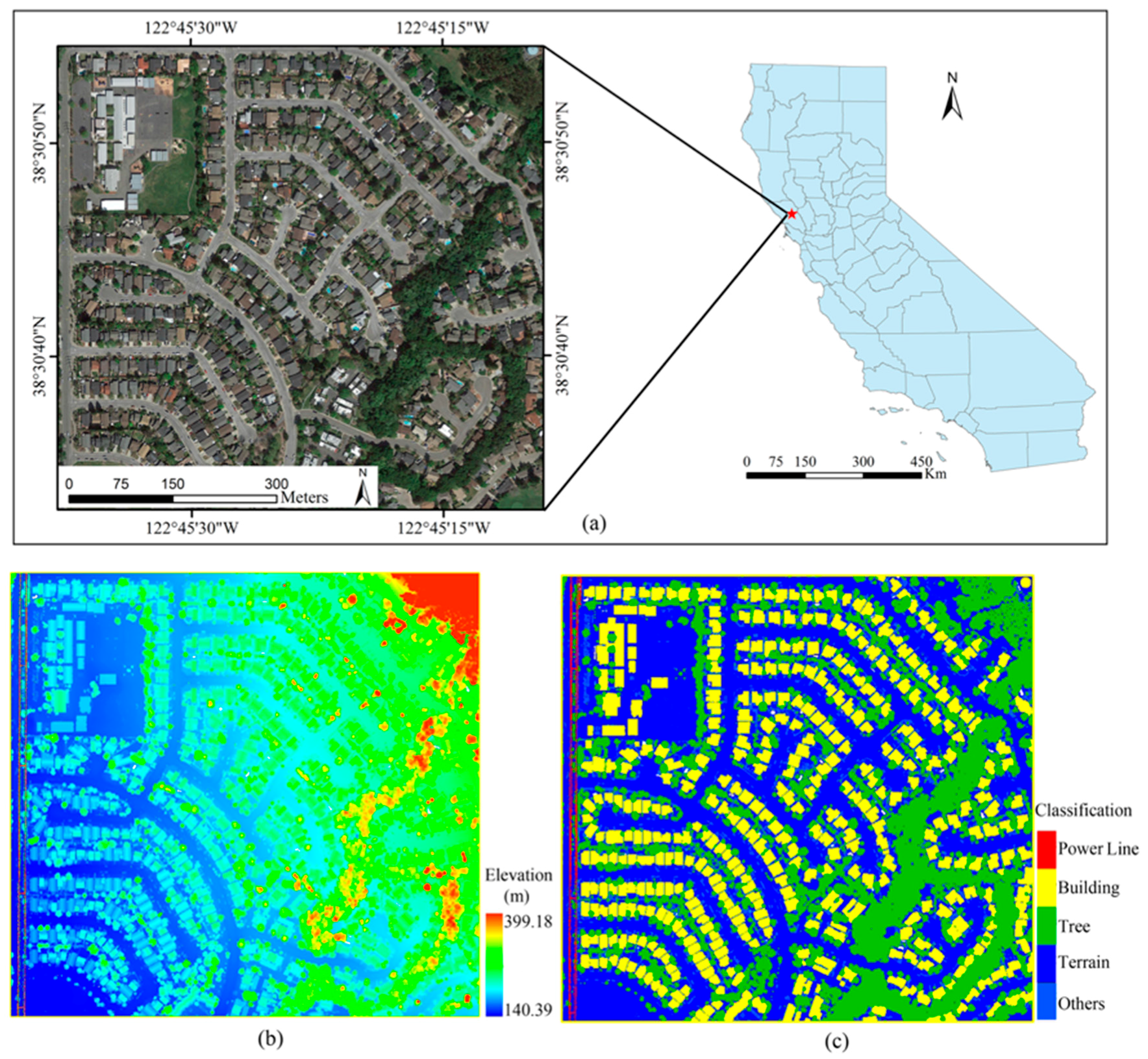
The study area is located in Santa Rosa, CA, USA (38°30′N, 122°45′W), covering an area of about 700 m 650 m (Figure 1). The elevation of the study area varies from 140 m to 399 m. Within the study area, the major land cover types are buildings, trees, pavement, bare soil, water bodies, power lines, shrubs, and grassland. The airborne LiDAR dataset covering the study area was provided by the University of Maryland and the Sonoma County Vegetation Mapping and LiDAR Program under grant NNX13AP69G from NASA’s Carbon Monitoring System. This dataset was collected in 2013 using two LiDAR systems, one carrying a Leica ALS50 and the other a Leica ALS70. The systems flew at 900 m above the ground with a 30° field of view (FOV), and recorded up to 5 echoes per pulse. The average swath width of a single pass was around 400 m with about 50% swath overlap. In total, 4,615,428 points were collected, and the average point density was 10.14 pts/m2.
In order to evaluate the classification accuracy, we semi-automatically generated ground truth classes using the software TerraScanTM with the aid of a high-resolution orthophoto from GoogleTM Earth. The five ground truth classes consisted of buildings, trees, power lines, terrain (merging pavement, bare soil, and grassland), and others (including shrubs and cars).
2.2. Features of Interest
In the present study, four kinds of features were used in the classification, including height-based features, eigen-based features, echo-based features, and multi-scale features.
2.2.1. Height-Based Features
A significant breakthrough of the LiDAR sensor is the ability to acquire highly accurate height information. LiDAR-derived height data, such as digital surface models (DSM), digital elevation models (DEM), and normalized DSM (nDSM) can make it possible to identify certain objects [1,31,32], such as low vegetation and terrain in urban area [5,33]. In this study, the normalized height (denoted as ) representing the height value in nDSM and the height variance (denoted as ) in a local spherical neighborhood were applied in the classification. The first step for extracting the normalized height is to identify the ground points. This procedure was performed using a progressive triangulated irregular network (TIN) densification filtering algorithm as implemented in the software LAStools [34]. Then, we used the ordinary Kriging method to interpolate 1 m DSM and DEM from the first returns and ground returns, respectively, and calculated the nDSM as the difference between DSM and DEM following standard industrial procedure. The height variance was repeatedly computed at multiple scales as described in Section 2.2.4.
2.2.2. Eigen-Based Features
Eigen-based features are effective estimators for the local spatial distribution of a set of points. Given a set of n 3D points within a spherical neighborhood, the covariance matrix can be calculated using the following equation:
where is the mean of the points, i.e., . The eigenvectors () and eigenvalues () can be derived using the eigen-decomposition method, which is shown in Equation (2).
In geometry, eigenvectors are associated with the normal vector and coefficients of the best-fitting plane for the points within the local neighborhood, and eigenvalues are helpful to measure whether the points are linearly, planarly, or spherically distributed [35]. Therefore, eigen-based features derived from the eigenvectors and eigenvalues can contribute to the improvement of classification accuracy in urban areas [10,36]. In this experiment, we derived two eigen-based features from the eigenvectors to aid in the classification, i.e., corresponding to the angle between the local normal vector and the vertical direction, and corresponding to the residual of the local plane fitting. We also derived four eigen-based features, linearity , planarity , sphericity , and change of curvature k, from the eigenvalues following the definitions in Chehata et al. (2009) [6] and Ni et al. (2017) [37], i.e., , , and .
2.2.3. Echo-Based Features
Due to the diversity of illuminated surfaces, the emission pulses from a LiDAR sensor may indicate different backscatter characteristics. Generally, the laser pulse can penetrate the canopy of vegetation and hence the points of canopy will indicate multiple returns, whereas terrain and buildings are commonly recorded as a single return. Therefore, the information on different objects can be revealed from the number of returns [38,39]. In this study, two echo-based features were selected for the classification, i.e., corresponding to the total number of echoes, and corresponding to the ratio of the echo number to .
2.2.4. Multi-Scale Features
As stated above, most of our features aimed to measure the local geometric characteristics of points within a spherical neighborhood. The radius r of the spherical neighborhood determines a certain scale at which the local distribution characteristics will be measured. Recent research has demonstrated that different local distribution characteristics will be obtained via a series of r [40]. For example, at the scale of a few centimeters, points belonging to power-lines distribute like a 1D line, whereas those belonging to trees distribute like a mixture of 1D branches and 2D leaves. At a larger scale such as 3 m, the points belonging to power-lines still distribute like a 1D line, while those belonging to trees now indicate a scattered distribution in 3D space. Combinations of the distribution characteristics at different scales can provide effective information to discriminate between different classes.
In order to evaluate the local geometric characteristics under different scales, the features stated in the previous section including , , , , k, , and were repeatedly computed at each scale of interest. Taking into account the point density and the object size in the study area, we empirically determined the scales as 1.5 m, 2.5 m, and 3.5 m. Practically, the points near the object boundaries may have too few neighborhoods to evaluate valid feature values at a small scale. In that case, the feature values in the closest available larger scale were used to complete the missing values.
2.3. Classification Schemes
2.3.1. PBL-BP Classification
PBL is a general one-class classification scheme that models the probability of an individual sample x being positive (denoted as ) from the input positive and unlabeled training samples. Due to the absence of reliable negative samples, traditional supervised learning methods are inefficient for doing this. Let denote that x is collected as a labeled sample and denote that x is collected as an unlabeled sample. Then, the model trained using positive and unlabeled data can be denoted as , where refers to the presence-background strategy. According to the conditional probability method and the random sampling strategy, the quantitative relationship between the trained model and the desired model can be expressed as:
where c is a constant that can be estimated from validation data O. In practice, a reliable way to estimate c is to average the predicted probabilities for all :
where n is the cardinality of dataset O.
In summary, the main idea behind the PBL method is to generate a desired model in two steps. Firstly, the initial probability is predicted by a binary classifier that is trained using positive and unlabeled samples. Then, the desired model can be generated by calibrating the initial probability with a constant c, which is estimated from validation data, through a non-linear transformation. It is worth mentioning that PBL is not a specific classifier, but a general framework that can be implemented by any classifier that is able to correctly predict the conditional probability. More details about the PBL algorithm can be found in Li et al. (2011) [30].
Since the back propagation (BP) neural network can correctly evaluate the posterior probability [41,42], in this study PBL-BP was applied to perform the classification. Two hidden layers were used during the training of the BP neural network, and the transfer functions were tan-sigmoid and log-sigmoid, respectively. The number of nodes in hidden layers was determined empirically. For each class, we randomly selected 1000 positive samples and 5000 unlabeled samples. Then, the features of interest were extracted and normalized into the range [0, 1]. Note that we did not carry out the procedure of feature selection, hence the applied features shared the same weights during the process of training. Additionally, we extracted 75% of the collected samples to train the classifier, and 25% as validation data to estimate the constant c. Given that the initial synaptic weights are randomly determined, the output of the BP neural network will be different for each case. In order to achieve a reliable model, the BP neural network was trained ten times with the same network structure, parameters, and training data. Afterwards, these outputs were averaged to construct the final decision model.
We also used PBL-BP to produce a multi-class classification result through a one-against-all strategy [43]. The PBL-BP algorithm was independently performed for each class, and the outputs of posterior probabilities were combined. Afterwards, each sample was labeled as the class corresponding to the maximum posterior probability.
2.3.2. Other One-Class Classification Methods
Besides the PBL-BP algorithm, this study also classified the LiDAR data in the study area using the OCSVM, BSVM, and MaxEnt algorithms. Classification results from these methods were quantitatively compared with those of PBL-BP, so as to comprehensively evaluate the effectiveness of PBL-BP in the extraction of a single class from LiDAR point clouds.
The OCSVM algorithm was implemented in the LIBSVM package released by Chang and Lin (2001) [44]. OCSVM requires only positive samples as a training set, irrespective of negative and unlabeled samples. We used the Gaussian radial basis function (RBF) kernel to facilitate dealing with the high-dimension features [12,45]. Two parameters needed to be determined during the training: the RBF kernel width γ and the rejection fraction ʋ. Following the guideline of LIBSVM, we evaluated γ ranges from 2−10, 2−9, …, 210 and ʋ ranges from 0.1, 0.2, …, 0.9. In view of the fact that OCSVM normally encounters the over-fitting problem, we randomly selected 750 positive samples per class for generating the classifier, and applied both positive and negative data for validation, so as to achieve the best performance.
The BSVM algorithm was implemented in the SVMlight package [46]. For the same reason as with the OCSVM algorithm, we chose the Gaussian RBF kernel to build the desired model. For each class, 1000 positive samples and 5000 unlabeled samples were randomly collected. The training process included the determination of three parameters: the RBF kernel width γ, the weights of negative errors c, and the factor j representing the bias of weight between positive errors and negative errors. In our experiment, we manually set γ from 2−4, 2−3, …, 24, c from 2−7, 2−3, …, 20, and j from 21, 22, …, 26. According to the empirical approach proposed by Liu et al. (2003) [14] and Li et al. (2011) [30], we extracted 75% of the collected samples as training data and 25% as validation data, and performed classifier selection criterion to evaluate the best γ, c and j. Afterwards, we used these parameters together with the initial training set to generate the final decision model.
The MaxEnt algorithm was implemented using the MAXENT software [47]. We randomly selected 1000 positive samples and 5000 unlabeled samples for each class and extracted 75% of them as training data. To reduce over-fitting, the regularization multiplier was set to 2.00 [29]. The outputs of MaxEnt are logistic values; hence, a threshold is required to convert the output values into binary classes. Following the guidelines in [26,28], we extracted 25% of the selected samples as validation data, and set the threshold as the logistic value, which is equivalent to a 5% omission rate of the validation data. Other user-defined parameters were set to the default values.
2.3.3. SVM Classification
To systematically investigate the performance of PBL-BP, we compared its multi-class classification results with that from the SVM method, which was implemented by LIBSVM package. SVM solves the classification problem by seeking optimal separating hyperplanes that maximize the distances between different classes, and is extensively used in remote sensing analysis [48,49]. For non-linearly separable problems, the kernel function is introduced to transform the original samples into a high dimensional feature space where the samples can be linearly separated. In this experiment, an RBF kernel was used since it has proved to be effective in LiDAR point cloud classification [10,36,50].
The input for SVM consisted of the training samples of all classes. For each class, 1000 training samples were randomly collected in the study area. Two parameters were involved in the training of the classifier: the RBF kernel width γ and the penalty parameter C. We evaluated both γ and C in the range of 2−10, 2−9, …, 210 using 5-fold cross-validation [51]. Afterwards, the evaluated parameters were used to perform the classification.
2.4. Accuracy Assessment
The classification results were quantitatively evaluated based on the ground truth classes using a confusion matrix, which is widely applied in the performance assessment of an algorithm [44]. In the confusion matrix, true positive (TP) denotes the number of correctly labeled positive samples, and true negative (TN) denotes the number of correctly labeled negative samples. Meanwhile, false positive (FP) refers to the number of negative samples that were incorrectly labeled as positive samples, and false negative (FN) refers to the number of positive samples that were incorrectly labeled as negative samples. From the confusion matrix, we can calculate the producer’s accuracy (PA), which represents the probability of a sample belonging to a specific class was correctly labeled, the user’s accuracy (UA), which measures the correct rate of the samples that were labeled as a specific class, and overall accuracy (OA), which indicates the proportion of correctly classified samples among the total number of samples. In one-class classification problems, a high OA is not necessarily equivalent to an accurate result for a specific class, whereas UA and PA are necessarily to be high for an accurate classification [15,52,53]. Therefore, we used the F-score, which is defined as the harmonic mean of UA and PA, for assessing the accuracies of one-class classification results. The PA, UA, OA, and F-score can be derived as follows:
3. Results
3.1. One-Class Classification Results
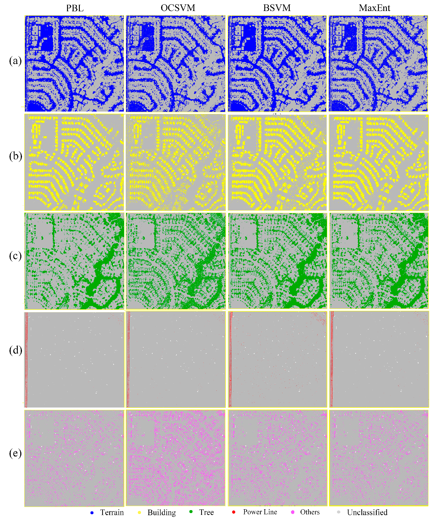
Figure 2 illustrates the one-class classification results of PBL-BP, OCSVM, BSVM and MaxEnt for each class in the study area. Accuracy assessment using ground truth classes revealed that the PBL-BP algorithm successfully extracted all of the classes in the scene (Table 1). The highest accuracies were obtained in the classification of terrain, with an F-score of 0.98. Both PA and UA for terrain were high (98.04% and 98.10%, respectively). A small number of trees were incorrectly classified as power lines, and the mislabeled points for buildings were mainly distributed within the gable roofs that showed similar features to trees. There was confusion between trees and shrubs in the classification map, and the F-score of trees (0.92) was relatively lower than those of the other classes. The mean F-score for all of the classes from the PBL-BP classification results was 0.94, indicating that the results had high agreement with ground truth classes.
Quantitative assessment of the classification results indicated that PBL-BP outperformed the other one-class classifiers (Table 1). In general, OCSVM produced lots of salt and pepper noise in the classification maps. Both OCSVM and BSVM obtained poor classification results for class other since many instances of trees and terrain were wrongly labeled as belonging to that class. There was a significant confusion between power lines and trees in the BSVM classification map. The mean F-scores for all of the classes from the classification results of OCSVM and BSVM were 0.68 and 0.82, which were 0.26 and 0.12 lower than those from PBL-BP, respectively. The classification maps of MaxEnt and PBL-BP were similar, with mean F-scores of 0.93 and 0.94, respectively.
3.2. Multi-Class Classification Results
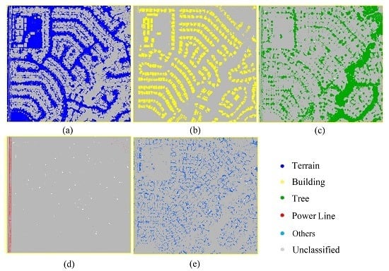
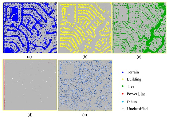
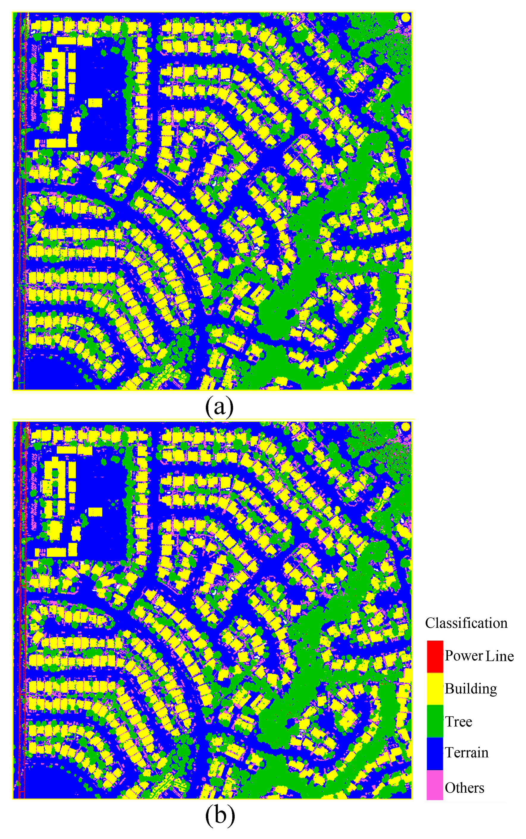
PBL-BP produced a multi-class classification result (Figure 3a) with an OA of 96.97% (Table 2). When compared with the one-class classification results, the error of power line decreased, while the omission of the power line increased since the pylons tended to be classified as trees. There were mainly two types of error in the multi-class classification map: (1) a large number of points belonging to class other (approximately 10.1%) were incorrectly classified as terrain and trees; and (2) some small objects on building roofs were incorrectly classified as trees.
Figure 3b shows the classification results of SVM. As can be seen, its classification map was very similar to PBL-BP, and both results showed a high consistency with the ground truth data. The quantitative assessment of the classification results is given in Table 3. SVM obtained high PAs for all classes, while the UAs for classes other and power lines were low (69.30% and 84.75%, respectively). The OA of PBL-BP was 96.97%, whereas that of SVM was 96.07%, indicating that PBL-BP achieved slightly better results than SVM.
4. Discussion
One outcome of interest from this research is the effectiveness of PBL-BP algorithm for the one-class classification of a LiDAR point cloud. According to our experimental results, methods learning from both positive and unlabeled samples (PBL-BP, MaxEnt and BSVM) commonly yielded more accurate results than those learning from only positive samples (OCSVM). This is consistent with findings reported by Castelli et al. (1996) [54], who concluded that unlabeled samples can provide useful information to improve classification accuracy. In the classification, BSVM achieved high PAs, but the UAs were commonly low, indicating that BSVM cannot effectively solve the over-fitting problem. A possible reason for this may be the difficulties in tuning free parameters. BSVM weights the unlabeled samples to construct a reliable decision rule, but the weights are hard to tune as there is no direct approach to evaluate the actual rate of noises in the unlabeled data [19]. MaxEnt is one of the state-of-the-art methods learning from positive and unlabeled samples, and achieved high accuracies in the classification. However, it suffers from several drawbacks. One major drawback of MaxEnt is that its outcome depends critically on the input parameters [55,56]. Additionally, assuming a distribution model of the data can sometimes be problematic [29]. Our experiment results indicated that MaxEnt outperformed BSVM, which is different from the findings reported by Mack and Waske (2017) [57] and Stenzel et al. (2017) [58]. This phenomenon might have resulted from the different thresholds that were used to transform the model outputs into binary classes. Studies have found that the default threshold performed relatively poorly as compared with a threshold obtained from alternative threshold selection strategies, and might be insufficient to balance false positive and false negative classifications [17,57]. Although threshold selection strategies can improve the classification results, the addition of such a procedure has the disadvantage of increasing the complexity of model selection. By contrast, PBL does not involve complicated parameter tuning and model selection, and can produce more reliable and accurate classification results than the other one-class classifiers. Therefore, PBL is very promising for solving one-class classification problems of LiDAR data.
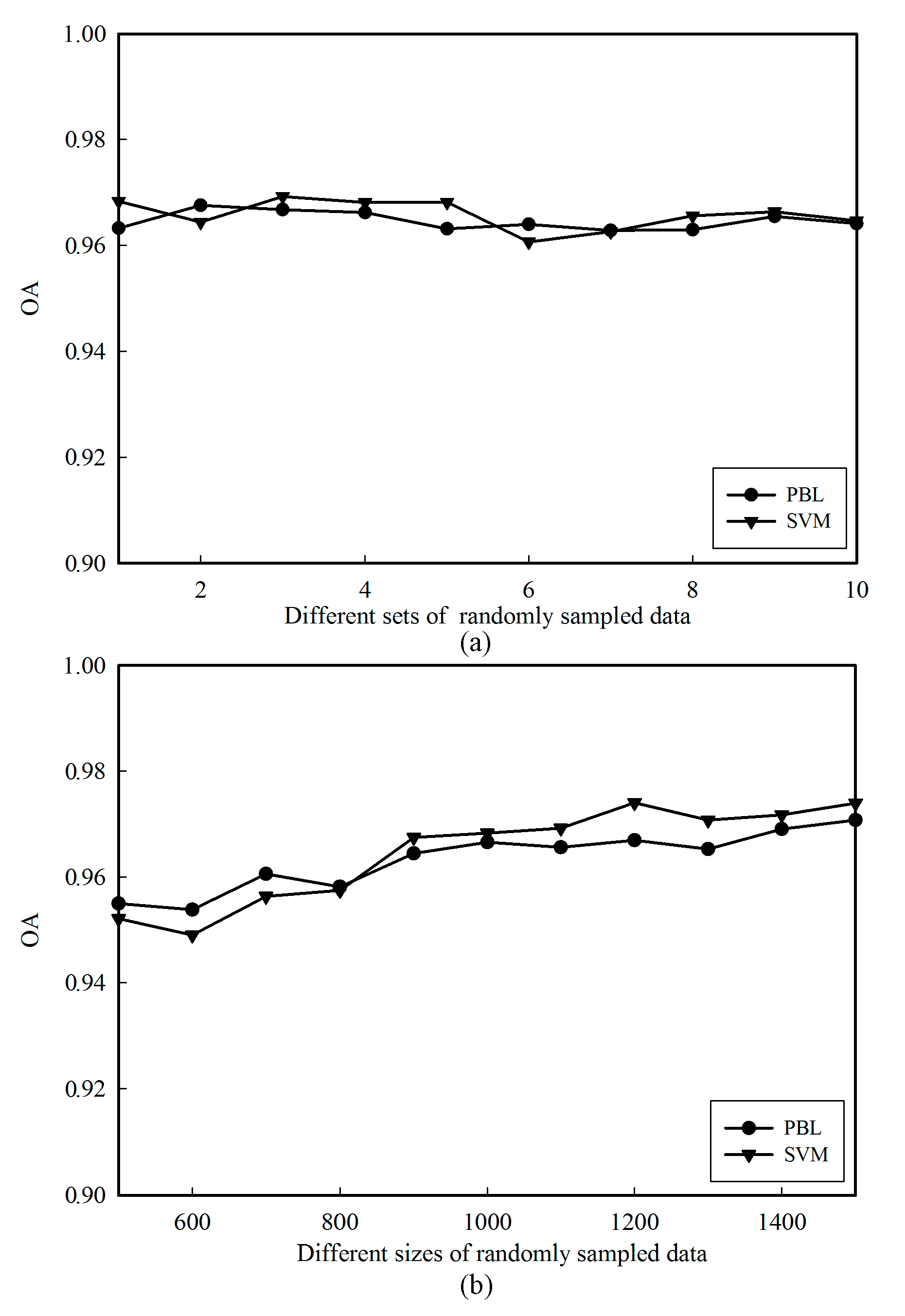
In addition, this study revealed the potential of the PBL-BP algorithm in multi-class classification of LiDAR point cloud, for the first time. Previous findings have indicated that the classification accuracy can be influenced greatly by the training samples [49,59]. To provide more information on the performance of PBL-BP, comparative experiments were conducted from two aspects: (1) training sets, and (2) sample sizes. To evaluate the impact of training sets on the classification results, we ran PBL-BP and SVM ten times using different randomly sampled training data. In terms of sample sizes, we trained PBL-BP and SVM with different sizes of randomly sampled data. The sizes of training samples for each class were in the range of [500, 1500], incrementing 100 samples each time. The classification results (Figure 4) demonstrate that both of their OAs tend to increase with the sample sizes, which is consistent with findings reported in [59]. Although PBL-BP provided a slightly lower mean OA when compared with SVM (96.39% and 96.51%, respectively), the differences are very small (approximately 0.12%). Therefore, it is reasonable to conclude that the PBL-BP algorithm can provide a comparable performance to the SVM method.
PBL can be particularly useful in practical applications where the extraction of a specific class is needed. Although traditional supervised classification methods can be used to achieve this goal, the adoption of such methods requires training samples of all classes in the study area, which are commonly highly labor-intensive and time-consuming to collect. The cost of acquiring training samples for classes of no interest may be very high, especially for urban scenes that contain a variety of objects [60]. Meanwhile, traditional supervised classification methods are normally focused on the overall classification accuracy rather than the class of interest [45,61]. However, maximizing the overall classification accuracy is not necessarily equivalent to optimizing the accuracy of a specific class [49]. In contrast, PBL is focused tightly on the specific class of interest, and requires only the positive and unlabeled samples for training. It is not necessary to collect any negative samples and hence the cost of collecting training data can be significantly reduced. Since PBL can reduce the requirement for training data without any substantial loss in accuracy, it may be a better choice to classify a specific class of interest from LiDAR data as compared with traditional supervised classification methods.
Previous research has demonstrated that the selection of the classifier is critical to the successful classification of complex urban scenes and the optimum choice will vary with different data [49]. In other words, the performance of classifiers is data-dependent, and one classifier might be able to handle some specific datasets but be incapable of dealing with other datasets [62]. Since it is hard to choose a best classifier in a practical classification task, ensemble methods that combine the predictions of several individual classifiers have become a new prospect for improving classification results [8,9,63,64]. However, predictions resulted by different classifiers are less comparable, hence an appropriate rule is needed to combine them [65,66]. PBL is a flexible framework that can calibrate the initial predictions of any binary classifiers through a non-linear transformation. After the calibration, the predictions become uniform and comparable and hence can be combined to generate the decision model. Therefore, PBL may also be useful in applications where ensemble classifications are to be carried out, which will be further investigated in the near future.
The PBL is based on the assumption that samples are selected completely in random. In other words, positive training samples are randomly collected from all positive data, and unlabeled training samples are randomly collected from the whole study area. In a real-world application, however, a commonly used method of collecting training samples is to visually estimate the classes and draw polygons around the areas covering a number of training samples, which will lead to a strong spatial autocorrelation in the training data. In such cases, the training samples are highly clustered and this assumption may not be satisfied. Moreover, studies have found that the purity and quality of positive samples and the proportion of positive samples to unlabeled samples are important factors that influence PUL classification accuracy [22]. Although the theoretical principles underlying PUL and PBL are similar, a more reliable sampling design is adopted in PBL [30]. Therefore, the effect of these factors on PBL classification results is still unclear. Further study is still needed to identify how biases and errors of training samples collection influence the PBL classification results.
5. Conclusions
This study investigated the classification of LiDAR data using a novel one-class classification method, i.e., PBL algorithm. The classification result was systematically compared with OCSVM, BSVM, and MaxEnt to evaluate the performance of PBL-BP in the extraction of a single class (e.g., buildings, trees, terrain, power lines and other) in an urban area. The PBL classification results had high agreement with the ground truth classes, with a mean F-score of 0.94 for all classes, which was 0.26 and 0.12 higher than the results from OCSVM and BSVM, respectively. The results also demonstrated that PBL outperformed the state-of-the-art MaxEnt method, while significantly reducing the effort in parameter tuning and model selection.
Moreover, this study estimated the performance of PBL in multi-class classification with different training sets and sample sizes. Results implied that PBL can produce comparable accuracy with SVM with an OA of above 96%, and hence shows great potential for LiDAR point cloud classification, especially when the training classes are incomplete. Future studies will be focused on the use of PBL in generating an ensemble model to further improve the classification accuracy. The influence of sampling biases and errors on the classification results also needs to be further studied.
Acknowledgments
We acknowledge the University of Maryland and the Sonoma County Vegetation Mapping and LiDAR Program for providing the LiDAR data. We are grateful to the editor and the anonymous reviewers for their insightful suggestions on this work.
Author Contributions
Zurui Ao, Wenkai Li and Qinghua Guo designed the experiment; Zurui Ao performed the experiment and analyzed the results. Zurui Ao, Yanjun Su, Qinghua Guo and Jing Zhang contributed towards writing the manuscript.
Conflicts of Interest
The authors declare no conflict of interest.
References
- Niemeyer, J.; Rottensteiner, F.; Soergel, U. Contextual classification of LiDAR data and building object detection in urban areas. ISPRS J. Photogramm. Remote Sens. 2014, 87, 152–165. [Google Scholar] [CrossRef]
- Tian, S.; Zhang, X.; Tian, J.; Sun, Q. Random forest classification of wetland landcovers from multi-sensor data in the arid region of Xinjiang, China. Remote Sens. 2016, 8, 954. [Google Scholar] [CrossRef]
- Su, Y.; Guo, Q.; Collins, B.M.; Fry, D.L.; Hu, T.; Kelly, M. Forest fuel treatment detection using multi-temporal airborne LiDAR data and high-resolution aerial imagery: A case study in the sierra nevada mountains, California. Int. J. Remote Sens. 2016, 37, 3322–3345. [Google Scholar] [CrossRef]
- Wu, B.; Yu, B.; Wu, Q.; Yao, S.; Zhao, F.; Mao, W.; Wu, J. A graph-based approach for 3d building model reconstruction from airborne LiDAR point clouds. Remote Sens. 2017, 9, 92. [Google Scholar] [CrossRef]
- Charaniya, A.P.; Manduchi, R.; Lodha, S.K. Supervised Parametric Classification of Aerial LiDAR Data. In Proceedings of the CVPRW, Washington, DC, USA, 27 June–2 July 2004; p. 30. [Google Scholar]
- Chehata, N.; Guo, L.; Mallet, C. Airborne LiDAR feature selection for urban classification using random forests. Int. Arch. Photogramm. Remote Sens. 2009, 38, 207–212. [Google Scholar]
- Alexander, C.; Tansey, K.; Kaduk, J.; Holland, D.; Tate, N.J. Backscatter coefficient as an attribute for the classification of full-waveform airborne laser scanning data in urban areas. ISPRS J. Photogramm. Remote Sens. 2010, 65, 423–432. [Google Scholar] [CrossRef]
- Lodha, S.K.; Fitzpatrick, D.M.; Helmbold, D.P. Aerial LiDAR Data Classification Using Adaboost. In Proceedings of the 3DIM, Montreal, QC, Canada, 21–23 August 2007; pp. 435–442. [Google Scholar]
- Guo, B.; Huang, X.; Zhang, F.; Sohn, G. Classification of airborne laser scanning data using jointboost. ISPRS J. Photogramm. Remote Sens. 2015, 100, 71–83. [Google Scholar] [CrossRef]
- Mallet, C.; Bretar, F.; Roux, M.; Soergel, U.; Heipke, C. Relevance assessment of full-waveform LiDAR data for urban area classification. ISPRS J. Photogramm. Remote Sens. 2011, 66, S71–S84. [Google Scholar] [CrossRef]
- Zhou, M.; Li, C.; Ma, L.; Guan, H. Land cover classification from full-waveform LiDAR data based on support vector machines. Int. Arch. Photogramm. Remote Sens. Spat. Inf. Sci. 2016, XLI-B3, 447–452. [Google Scholar]
- Schölkopf, B.; Platt, J.C.; Shawe-Taylor, J.; Smola, A.J.; Williamson, R.C. Estimating the support of a high-dimensional distribution. Neural Comput. 2001, 13, 1443–1471. [Google Scholar] [CrossRef] [PubMed]
- Zhang, J.; Li, P.; Wang, J. Urban built-up area extraction from landsat TM/ETM+ images using spectral information and multivariate texture. Remote Sens. 2014, 6, 7339–7359. [Google Scholar] [CrossRef]
- Liu, B.; Dai, Y.; Li, X.; Lee, W.S.; Yu, P.S. Building Text Classifiers Using Positive and Unlabeled Examples. In Proceedings of the ICDM, Melbourne, FL, USA, 22 November 2003; pp. 179–186. [Google Scholar]
- Baldeck, C.A.; Asner, G.P. Single-species detection with airborne imaging spectroscopy data: A comparison of support vector techniques. IEEE J. STARS 2015, 8, 2501–2512. [Google Scholar] [CrossRef]
- Liu, Z.; Shi, W.; Li, D.; Qin, Q. Partially supervised classification: based on weighted unlabeled samples support vector machine. Int. J. Data Warehous. 2008, 2, 42–56. [Google Scholar] [CrossRef]
- Mack, B.; Roscher, R.; Waske, B. Can I Trust My One-Class Classification. Remote Sens. 2014, 6, 8779–8802. [Google Scholar] [CrossRef]
- Elkan, C.; Noto, K. Learning Classifiers from Only Positive and Unlabeled Data. In Proceedings of the 14th ACM SIGKDD International Conference on Knowledge Discovery and Data Mining, Las Vegas, NV, USA, 24–27 August 2008; pp. 213–220. [Google Scholar]
- Li, W.; Guo, Q.; Elkan, C. A positive and unlabeled learning algorithm for one-class classification of remote-sensing data. IEEE Trans. Geosci. Remote Sens. 2011, 49, 717–725. [Google Scholar] [CrossRef]
- Guo, Q.; Li, W.; Liu, D.; Chen, J. A framework for supervised image classification with incomplete training samples. Photogramm. Eng. Remote Sens. 2012, 78, 595–604. [Google Scholar] [CrossRef]
- Wan, B.; Guo, Q.; Fang, F.; Su, Y.; Wang, R. Mapping us urban extents from modis data using one-class classification method. Remote Sens. 2015, 7, 10143–10163. [Google Scholar] [CrossRef]
- Chen, X.; Yin, D.; Chen, J.; Cao, X. Effect of training strategy for positive and unlabeled learning classification: Test on Landsat imagery. Remote Sens. Lett. 2016, 7, 1063–1072. [Google Scholar] [CrossRef]
- Jaynes, E.T. Information theory and statistical mechanics. Phys. Rev. 1957, 106, 620. [Google Scholar] [CrossRef]
- Phillips, S.J.; Dudík, M.; Schapire, R.E. A Maximum Entropy Approach to Species Distribution Modeling. In Proceedings of the Twenty-First International Conference on Machine Learning, Banff, AB, Canada, 4–8 July 2004; p. 83. [Google Scholar]
- Phillips, S.J.; Anderson, R.P.; Schapire, R.E. Maximum entropy modeling of species geographic distributions. Ecol. Model. 2006, 190, 231–259. [Google Scholar] [CrossRef]
- Li, W.; Guo, Q. A maximum entropy approach to one-class classification of remote sensing imagery. Int. J. Remote Sens. 2010, 31, 2227–2235. [Google Scholar] [CrossRef]
- Baldwin, R.A. Use of maximum entropy modeling in wildlife research. Entropy 2009, 11, 854–866. [Google Scholar] [CrossRef]
- Merow, C.; Smith, M.J.; Silander, J.A. A practical guide to MaxEnt for modeling species’ distributions: What it does, and why inputs and settings matter. Ecography 2013, 36, 1058–1069. [Google Scholar] [CrossRef]
- Radosavljevic, A.; Anderson, R.P. Making better MaxEnt models of species distributions: Complexity, overfitting and evaluation. J. Biogeogr. 2014, 41, 629–643. [Google Scholar] [CrossRef]
- Li, W.; Guo, Q.; Elkan, C. Can we model the probability of presence of species without absence data? Ecography 2011, 34, 1096–1105. [Google Scholar] [CrossRef]
- Bretar, F.; Chauve, A.; Bailly, J.-S.; Mallet, C.; Jacome, A. Terrain surfaces and 3d landcover classification from small footprint full-waveform LiDAR data: Application to badlands. Hydrol. Earth Syst. Sci. 2009, 13, 1531–1544. [Google Scholar] [CrossRef]
- Huang, Y.; Yu, B.; Zhou, J.; Hu, C.; Tan, W.; Hu, Z.; Wu, J. Toward automatic estimation of urban green volume using airborne LiDAR data and high resolution remote sensing images. Front. Earth Sci. 2013, 7, 43–54. [Google Scholar] [CrossRef]
- Zhu, X.; Toutin, T. Land cover classification using airborne LiDAR products in Beauport, Québec, Canada. Int. J. Image Data Fusion 2013, 4, 252–271. [Google Scholar] [CrossRef]
- LAStools-Efficient Tools for LiDAR Processing, Version 140430. 2014. Available online: https://rapidlasso.com/lastools/ (accessed on 6 August 2017).
- Lin, C.-H.; Chen, J.-Y.; Su, P.-L.; Chen, C.-H. Eigen-feature analysis of weighted covariance matrices for LiDAR point cloud classification. ISPRS J. Photogramm. Remote Sens. 2014, 94, 70–79. [Google Scholar] [CrossRef]
- Zhang, J.; Lin, X.; Ning, X. Svm-based classification of segmented airborne LiDAR point clouds in urban areas. Remote Sens. 2013, 5, 3749–3775. [Google Scholar] [CrossRef]
- Ni, H.; Lin, X.; Zhang, J. Classification of ALS point cloud with improved point cloud segmentation and random forests. Remote Sens. 2017, 9, 288. [Google Scholar] [CrossRef]
- Singh, K.K.; Vogler, J.B.; Shoemaker, D.A.; Meentemeyer, R.K. LiDAR-landsat data fusion for large-area assessment of urban land cover: Balancing spatial resolution, data volume and mapping accuracy. ISPRS J. Photogramm. Remote Sens. 2012, 74, 110–121. [Google Scholar] [CrossRef]
- Brennan, R.; Webster, T. Object-oriented land cover classification of LiDAR-derived surfaces. Can. J. Remote Sens. 2006, 32, 162–172. [Google Scholar] [CrossRef]
- Brodu, N.; Lague, D. 3D terrestrial LiDAR data classification of complex natural scenes using a multi-scale dimensionality criterion: Applications in geomorphology. ISPRS J. Photogramm. Remote Sens. 2012, 68, 121–134. [Google Scholar] [CrossRef] [Green Version]
- Richard, M.D.; Lippmann, R.P. Neural network classifiers estimate bayesian a posteriori probabilities. Neural Comput. 1991, 3, 461–483. [Google Scholar] [CrossRef]
- Yuan, H.; Van Der Wiele, C.F.; Khorram, S. An automated artificial neural network system for land use/land cover classification from landsat tm imagery. Remote Sens. 2009, 1, 243–265. [Google Scholar] [CrossRef]
- Allwein, E.L.; Schapire, R.E.; Singer, Y. Reducing multiclass to binary: A unifying approach for margin classifiers. J. Mach. Learn. Res. 2000, 1, 113–141. [Google Scholar]
- Chang, C.-C.; Lin, C.-J. LIBSVM: A library for support vector machines. ACM Trans. Intell. Syst. Technol. 2011, 2, 1–27. [Google Scholar] [CrossRef]
- Sanchez-Hernandez, C.; Boyd, D.S.; Foody, G.M. One-class classification for mapping a specific land-cover class: SVDD classification of fenland. IEEE Trans. Geosci. Remote Sens. 2007, 45, 1061–1073. [Google Scholar] [CrossRef]
- Joachims, T. Making large-Scale SVM Learning Practical. In Advances in Kernel Methods—Support Vector Learning; Schölkopf, B., Burges, C., Smola, A., Eds.; MIT-Press: Cambridge, MA, USA, 1999. [Google Scholar]
- Phillips, S.J. A Brief Tutorial on Maxent. 2017. Available online: http://biodiversityinformatics.amnh.org/open_source/maxent/ (accessed on 6 August 2017).
- Song, X.; Fan, G.; Rao, M. Svm-based data editing for enhanced one-class classification of remotely sensed imagery. IEEE Trans. Geosci. Remote Sens. Lett. 2008, 5, 189–193. [Google Scholar] [CrossRef]
- Foody, G.M.; Mathur, A.; Sanchez-Hernandez, C.; Boyd, D.S. Training set size requirements for the classification of a specific class. Remote Sens. Environ. 2006, 104, 1–14. [Google Scholar] [CrossRef]
- Luo, S.; Wang, C.; Xi, X.; Zeng, H.; Li, D.; Xia, S.; Wang, P. Fusion of airborne discrete-return LiDAR and hyperspectral data for land cover classification. Remote Sens. 2015, 8, 3. [Google Scholar] [CrossRef]
- Duan, K.; Keerthi, S.S.; Poo, A.N. Evaluation of simple performance measures for tuning svm hyperparameters. Neurocomputing 2003, 51, 41–59. [Google Scholar] [CrossRef]
- Foody, G. Thematic map comparison: Evaluating the statistical significance of differences in classification accuracy. Photogramm. Eng. Remote Sens. 2004, 70, 627–633. [Google Scholar] [CrossRef]
- Li, W.; Guo, Q. A New accuracy assessment method for one-class remote sensing classification. IEEE Trans. Geosci. Remote Sens. 2014, 52, 4621–4632. [Google Scholar]
- Castelli, V.; Cover, T.M. The relative value of labeled and unlabeled samples in pattern recognition with an unknown mixing parameter. IEEE Trans. Inf. Theory 1996, 42, 2102–2117. [Google Scholar] [CrossRef]
- Phillips, S.J. Transferability, sample selection bias and background data in presence-only modelling: A response to peterson et al. (2007). Ecography 2008, 31, 272–278. [Google Scholar] [CrossRef]
- Warren, D.L.; Seifert, S.N. Ecological niche modeling in MaxEnt: The importance of model complexity and the performance of model selection criteria. Ecol. Appl. 2011, 21, 335–342. [Google Scholar] [CrossRef] [PubMed]
- Mack, B.; Waske, B. In-depth comparisons of MaxEnt, biased SVM and one-class SVM for one-class classification of remote sensing data. Remote Sens. Lett. 2017, 8, 290–299. [Google Scholar] [CrossRef]
- Stenzel, S.; Fassnacht, F.E.; Mack, B.; Schmidtlein, S. Identification of high nature value grassland with remote sensing and minimal field data. Ecol. Indic. 2017, 74, 28–38. [Google Scholar] [CrossRef]
- Millard, K.; Richardson, M. On the importance of training data sample selection in random forest image classification: A case study in peatland ecosystem mapping. Remote Sens. 2015, 7, 8489–8515. [Google Scholar] [CrossRef]
- Silva, J.; Bacao, F.; Caetano, M. Specific land cover class mapping by semi-supervised weighted support vector machines. Remote Sens. 2017, 9, 181. [Google Scholar] [CrossRef]
- Silva, J.; Bacao, F.; Dieng, M.; Foody, G.M.; Caetano, M. Improving specific class mapping from remotely sensed data by cost-sensitive learning. Int. J. Remote Sens. 2017, 38, 3294–3316. [Google Scholar] [CrossRef]
- Liu, Y.; Guo, Q.; Tian, Y. A software framework for classification models of geographical data. Comput. Geosci. 2012, 42, 47–56. [Google Scholar] [CrossRef]
- Foody, G.; Boyd, D.; Sanchez-Hernandez, C. Mapping a specific class with an ensemble of classifiers. Int. J. Remote Sens. 2007, 28, 1733–1746. [Google Scholar] [CrossRef]
- Ko, C.; Sohn, G.; Remmel, T.K.; Miller, J. Hybrid ensemble classification of tree genera using airborne LiDAR data. Remote Sens. 2014, 6, 11225–11243. [Google Scholar] [CrossRef]
- Garg, A.; Pavlovic, V.; Huang, T.S. Bayesian Networks as Ensemble of Classifiers. In Proceedings of the IEEE 16th International Conference on Pattern Recognition, Quebec City, QC, Canada, 11–15 August 2002; Volume 2, pp. 779–784. [Google Scholar]
- Ko, C.; Sohn, G.; Remmel, T.K.; Miller, J.R. Maximizing the diversity of ensemble random forests for tree genera classification using high density LiDAR data. Remote Sens. 2016, 8, 646. [Google Scholar] [CrossRef]
Figure 1.
(a) The location and overview of the study area; (b) light detection and ranging (LiDAR) point cloud colored by point heights; (c) ground truth classes interpreted manually.
Figure 1.
(a) The location and overview of the study area; (b) light detection and ranging (LiDAR) point cloud colored by point heights; (c) ground truth classes interpreted manually.

Figure 2.
One-class classification results of presence and background learning algorithm implemented by back propagation neural network (PBL-BP), one-class support vector machines (OCSVM), biased SVM (BSVM) and maximum entropy (MaxEnt): (a) Terrain; (b) Building; (c) Tree; (d) Power Line; (e) Others.

Figure 3.
Multi-class classification results of presence and background learning algorithm implemented by back propagation neural network (PBL-BP) and support vector machine (SVM): (a) PBL-BP; (b) SVM.
Figure 3.
Multi-class classification results of presence and background learning algorithm implemented by back propagation neural network (PBL-BP) and support vector machine (SVM): (a) PBL-BP; (b) SVM.

Figure 4.
Comparison of overall accuracies (OAs) obtained from the presence and background learning algorithm implemented by back propagation neural network (PBL-BP) and support vector machine (SVM) using different randomly sampled training data: (a) different sets of randomly sampled data; (b) different sizes of randomly sampled data.


Table 1.
Accuracy assessment for One-class classification results of PBL-BP, OCSVM, BSVM and MaxEnt.
Table 1.
Accuracy assessment for One-class classification results of PBL-BP, OCSVM, BSVM and MaxEnt.
| Classes | Performance Metrics | PBL-BP | OCSVM | BSVM | MaxEnt |
|---|---|---|---|---|---|
| Terrain | UA (%) | 98.11 | 97.03 | 95.80 | 100.00 |
| PA (%) | 98.04 | 71.48 | 99.57 | 96.29 | |
| F-score | 0.98 | 0.82 | 0.97 | 0.98 | |
| Building | UA (%) | 94.03 | 70.56 | 82.94 | 86.17 |
| PA (%) | 90.63 | 79.72 | 96.79 | 98.57 | |
| F-score | 0.92 | 0.74 | 0.89 | 0.91 | |
| Tree | UA (%) | 96.01 | 66.26 | 82.92 | 87.56 |
| PA (%) | 92.49 | 74.59 | 98.09 | 97.38 | |
| F-score | 0.94 | 0.70 | 0.89 | 0.92 | |
| Power Line | UA (%) | 95.89 | 91.03 | 65.10 | 90.50 |
| PA (%) | 95.94 | 88.93 | 99.66 | 98.67 | |
| F-score | 0.96 | 0.89 | 0.78 | 0.94 | |
| Others | UA (%) | 91.73 | 16.18 | 45.49 | 86.48 |
| PA (%) | 92.00 | 48.81 | 82.89 | 98.22 | |
| F-score | 0.92 | 0.24 | 0.58 | 0.91 |
Table 2.
Confusion matrix for the PBL-BP multi-class classification result.
| Prediction | Terrain | Building | Tree | Power Line | Others | |
|---|---|---|---|---|---|---|
| Reference | ||||||
| Terrain | 2,301,098 | 37 | 792 | 0 | 1142 | |
| Building | 1396 | 917,961 | 49,115 | 7 | 3024 | |
| Tree | 5987 | 31,905 | 1,018,900 | 458 | 19,167 | |
| Power Line | 0 | 129 | 697 | 10,873 | 0 | |
| Others | 12,428 | 2795 | 10,582 | 3 | 226,807 | |
| PA (%) | 99.91 | 94.49 | 94.66 | 92.94 | 89.78 | |
| UA (%) | 99.15 | 96.34 | 94.33 | 95.87 | 90.67 | |
| OA (%) | 96.97 | |||||
Table 3.
Confusion matrix for support vector machine (SVM) classification result.
| Prediction | Terrain | Building | Tree | Power Line | Others | |
|---|---|---|---|---|---|---|
| Reference | ||||||
| Terrain | 2,241,724 | 0 | 5 | 0 | 61,340 | |
| Building | 0 | 935,627 | 27,062 | 89 | 8725 | |
| Tree | 11 | 31,467 | 1,008,098 | 2002 | 34,839 | |
| Power Line | 0 | 0 | 71 | 11,628 | 0 | |
| Others | 11,044 | 2319 | 2435 | 0 | 236,817 | |
| PA (%) | 97.34 | 96.31 | 93.65 | 99.39 | 93.75 | |
| UA (%) | 99.51 | 96.51 | 97.15 | 84.75 | 69.30 | |
| OA (%) | 96.07 | |||||
© 2017 by the authors. Licensee MDPI, Basel, Switzerland. This article is an open access article distributed under the terms and conditions of the Creative Commons Attribution (CC BY) license (http://creativecommons.org/licenses/by/4.0/).
Share and Cite
MDPI and ACS Style
Ao, Z.; Su, Y.; Li, W.; Guo, Q.; Zhang, J. One-Class Classification of Airborne LiDAR Data in Urban Areas Using a Presence and Background Learning Algorithm. Remote Sens. 2017, 9, 1001. https://doi.org/10.3390/rs9101001
AMA Style
Ao Z, Su Y, Li W, Guo Q, Zhang J. One-Class Classification of Airborne LiDAR Data in Urban Areas Using a Presence and Background Learning Algorithm. Remote Sensing. 2017; 9(10):1001. https://doi.org/10.3390/rs9101001
Chicago/Turabian StyleAo, Zurui, Yanjun Su, Wenkai Li, Qinghua Guo, and Jing Zhang. 2017. "One-Class Classification of Airborne LiDAR Data in Urban Areas Using a Presence and Background Learning Algorithm" Remote Sensing 9, no. 10: 1001. https://doi.org/10.3390/rs9101001
Note that from the first issue of 2016, this journal uses article numbers instead of page numbers. See further details here.