Validation of the Significant Wave Height Product of HY-2 Altimeter


1
National Ocean Technology Center, State Oceanic Administration, Tianjin 300112, China
2
National Satellite Ocean Application Service, State Oceanic Administration, Beijing 100081, China
3
Qingdao University, Qingdao 266003, China
*
Author to whom correspondence should be addressed.
Remote Sens. 2017, 9(10), 1016; https://doi.org/10.3390/rs9101016
Submission received: 14 August 2017
/
Revised: 22 September 2017
/
Accepted: 29 September 2017
/
Published: 30 September 2017
(This article belongs to the Special Issue Ocean Radar)
Abstract
:HY-2 was launched by China on August 2011, which has provided continuous wave height measurements to monitor ocean dynamic environments for more than 5 years. Before using these data, however, the measurements need to be validated. Based on the in situ buoy data from the National Data Buoy Center (NDBC) and the Jason-2 altimeter data, the HY-2 Ku-band significant wave height (SWH) measurements were validated. The comparisons showed that a linear regression with NDBC measurements can be used to improve the accuracy of the HY-2 SWH measurements. Compared with the NDBC SWH data, the validation results of the HY-2 SWH data show an RMS (root mean square) of 0.33 m, which is similar to that of the Jason-1 and Jason-2 data; the RMS of the HY-2 SWH is 0.30 m, which, corrected via linear regression, is similar to that of the corrected Jason-1 and Jason-2 data (0.27 m and 0.23 m, respectively). Therefore, the accuracy of the HY-2 SWH products is close to that of the Jason-1/2 SWH data.
1. Introduction
Traditional ocean wave observation is mainly performed via buoys, survey ships, and tide stations, and the coverage is very limited. These methods, however, cannot meet the needs of the current high-speed development of the economy and of scientific research. Altimetry effectively solves this problem, as it can provide large-scale, near-synchronous, high-spatial- and high-temporal-resolution observations. Altimeters have provided continuous wave height measurements for more than 20 years. Moreover, altimeter data have been widely used. The change from experimental ocean satellites to operational ocean satellites was significant [1]. Satellite altimeter operation benefits from continuously improving measurement accuracy and calibration and validation methods.
With the improvement of accuracy in altimeter observations and data processing methods, the altimeter data have been widely used in various fields, such as ocean circulation, ocean tides, middle scale eddies, upwelling currents, frontal eddies, and geodetic leveling [2,3]. Moreover, the application of altimeter SWH measurements to numerical ocean models has grown dramatically. The ERS-2 (since January 1996) and ENVISAT fast delivery altimeter SWH data were assimilated in ECMWF numerical wave models [4]. The positive impact of the satellite altimeter SWH data assimilation in numerical wave models has been estimated on the coastal scale or global scale [4,5,6]. Altimeter sea surface height anomaly (SSHA) data can be assimilated to the Princeton ocean model (POM), which improved the sea surface dynamic height and the results of the deep current field in the East China Sea [1]. The merged SWH data from HY-2, Jason-1/2, and ENVISAT can be used to analyze the characteristics of SWH in China’s seas and adjacent waters [7].
The success of assimilating multi-satellite data at global and regional scales depends upon two main conditions. The first one is the improvement of the accuracy of the altimeter observations and data processing methods. The second one is to determine the accuracy and the errors of the SWH measurements from various altimeters. Calibration and validation plans are usually conducted after operational satellite altimeters are launched. Based on these plans, these sea surface height (SSH), SWH, and backscattering coefficient measurements are calibrated and validated during dedicated commissioning phase operations [8,9]. Long-term monitoring of the quality of estimated geophysical parameters is then needed, since electronic drift and sensor degradations can affect the quality of measurements. The results of ENVISAT RA-2 wind and wave validation performed within the ESA RA-2 cross-calibration and validation team (CCVT) activities during the ENVISAT commissioning phase, as well as SWH and wind measurements from ERS-1/2, TOPEX/POSEIDON, and Jason-1/2, the results of long-term validation and proposed corrections, have been presented [9,10,11]. Since HY-2 was launched, there have been several published works evaluating HY-2 SWH accuracy; these works have consistently demonstrated its accuracy [12,13,14,15,16]. Some works focused on the preliminary calibration of HY-2 SWH shortly after its launch [7,12,13,17]. Some works focused on the HY-2 SWH correction method [15,16]. A conclusion can be drawn that HY-2 tends to overestimate the low sea state and underestimate wave heights throughout the remaining range of heights, especially for the high sea state [12,16]. The overall negative bias is 0.2 m and the RMS is 0.3 m [15]. All of these studies employed a 50 km spatial and 0.5 h temporal window for collocation, but the error caused by the spatial window was not discussed.
In this study, the HY-2 Ku band SWH data were validated by the SWH data from the NDBC buoy and cross-validated by Jason-2 Ku band SWH data for a long-term period. A linear regression formula was provided to ensure that the SWH data from HY-2A can work with other satellite altimetry data. Moreover, the uncertainty of HY-2 SWH measurements was estimated by coincident NDBC SWH measurements. Section 2 describes the data matching methods, statistics parameters, and the regression method used. Section 4 discusses the uncertainty of HY-2 SWH measurements and the error spatial variation. Finally, Section 5 states conclusions.
2. Materials and Methods
2.1. Materials
HY-2 was launched by China on 16 August 2011. It flies at an altitude of 971 km and an orbital inclination angle of 99.34°, an angle that allows for measurement closer to the poles. Its remote sensing loads include a microwave scatterometer, a radar altimeter, a scanning microwave radiometer, and a three-frequency microwave radiometer. The radar altimeter is used to detect the sea surface height (SSH), the SWH, and the sea surface wind speed (SSW).
In this paper, the HY-2 SWH data are Level 2 IGDR (interim geophysical data record) products distributed by the National Satellite Ocean Application Service (NSOAS), the State Oceanic Administration of China. The IGDR data mainly include the SWH, SSH, SSW, and relevant correction parameters, which were used to calculate the SSH. More than 4 years of HY-2 IGDR data (Cycle 1 to Cycle 110, from 1 October 2011 to 19 December 2015) are used here. During Cycle 40, the HY-2 satellite changes its altimeter sensor from the main one (Alt-A) to the backup one (Alt-B). Then, there are only 65 pass data in Cycle 40 (from Pass 1 to Pass 61) and only 305 pass data in Cycle 41 (from Pass 81 to Pass 386).
In order to validate the HY-2 Ku band SWH data, the Jason-2 data were collected for comparison. Jason-2 took over and continued the TOPEX/Poseidon and Jason-1 missions in 2008, in cooperation with CNES, Eumetsat, NASA, and NOAA. The Jason-2 has an orbit inclination angle of 66.04°, so all comparisons are located from 66.04° N to 66.04° S. In this paper, the Jason-2 SWH data are Level 2 GDR (geophysical data record) products distributed by CNES-AVISO. The Jason-2 altimeter data are collected from Cycle 119 to Cycle 268, a time span that is almost the same as that of the HY-2 data mentioned above. Data from both HY-2 and Jason-2 are used the Ku band SWH measurements.
The buoy data are generally assumed to be of high quality and have been used for validation altimeter SWH data [7,10,12,13,14,15,16,17,18,19,20]. The buoy data used here is regarded as “truth”; that is to say, any error is negligible. The buoy SWH data are obtained from the U.S. National Data Buoy Centre (NDBC), provided by NOAA, from October 2011 to 19 December 2015.
2.2. Methods
Using a spatial and temporal window, the collocation data set is established for the altimeter SWH validation. The ocean wave field varies temporally and spatially. Buoy measurements are the temporal variation of the wave field in a fixed buoy location; meanwhile, the altimeter measurements are the spatial variation in the wave field in a synchronous time. So the choice of the spatial and temporal window plays a key role in SWH validation, which can affect the final SWH accuracy.
Collocation criteria of 30 min for the temporal window and 50 km for the spatial window have been widely adopted since 1988 [19]. The validation of T/P, ENVISAT, Jason-1, and Jason-2 SWH measurements also used this criteria. In this paper, the spatial and temporal window is the same window used to compare the accuracy of the HY-2 altimeter with that of NDBC and Jason-2 in the SWH range of 0.5–11 m. For NDBC comparisons, the collocated data are selected when the distance approach of the altimeter ground track is less than 50 km, within a 0.5 h time window. Altimeter-collocated data are estimated as the distance between the altimeter and buoy is less than 50 km, and the along-track average of the altimeter data. For altimeter cross-comparisons, pairs of satellite data are selected when the time window selected as 0.5 h and 50 km each side of the crossing point, in order to filter time and space variability effects.
Results are presented as scatter plots and in tables, providing the number of data analyzed, the mean bias value, the RMS of HY-2 SWH and other altimeter or buoy SWH, the slope, and the intercept of the linear regression line between HY-2 SWH (x-axis) and other measurements (y-axis). Since the buoy/Jason-2 SWH data is treated as true, regressing the altimeter data onto the buoy data/Jason-2 is a good choice, regarding the HY-2 altimeter data as a dependent variable and the buoy/Jason-2 data as an independent variable. The slope and the intercept can eventually be used to directly correct the HY-2 SWH (the corrected SWH equals slope multiplied by measurement plus intercept).
3. Validation with NDBC and Jason-2
3.1. Validation with NDBC
There are more than 300 NDBC buoys, which can provide ocean wave data, but mostly near the coast. Thus, we first used the range between the buoy and the coast to filter the NDBC buoys. Excluding buoys that are too close to the coast, the buoys that range more than 50 km were kept down. Secondly, using the spatial-time window method mentioned in Section 2, the collocated NDBC buoys were attained. Finally, 50 NDBC buoys were found, which can be used to validate the HY-2 SWH products. The locations of the 50 buoys are shown in Figure 1.
The number of collocated data is 4838 for the NDBC comparisons within the 0.5 h time window and 50 km spatial window.
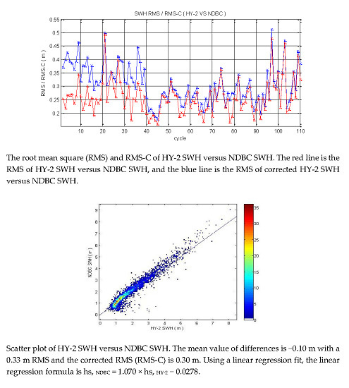
The accuracy of the HY-2 SWH is shown in Figure 2, Figure 3 and Figure 4, and statistical results are given in Table 1, Line 2. Compared with the NDBC buoy SWH, HY-2 SWH are lower in whole sea states, but in low sea states, the HY-2 SWH are higher.
The mean value of differences is −0.10 m with a 0.33 m RMS and the corrected RMS (RMS-C) is 0.30 m. Using a linear regression fit, the linear regression formula is hs, NDBC = 1.070 × hs, HY-2 − 0.0278. The linear regression corrected HY-2 SWH against NDBC SWH is shown in Table 1, Line 2, and the RMS from 0.33 to 0.30 m. The results of correction indicate that the linear regression formula is useful for increasing the accuracy of HY-2 altimeter SWH data.
3.2. Validation with JASON-2
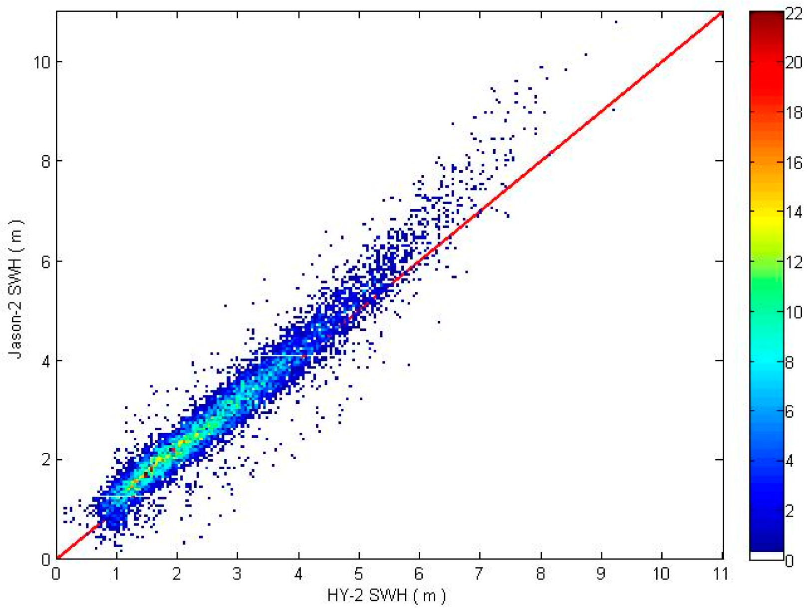
The number of collocated data is 8716 for the Jason-2 SWH comparisons (as shown in Figure 5) within the 0.5 h time window and the 50 km spatial window in the SWH range of 0.5–11 m.
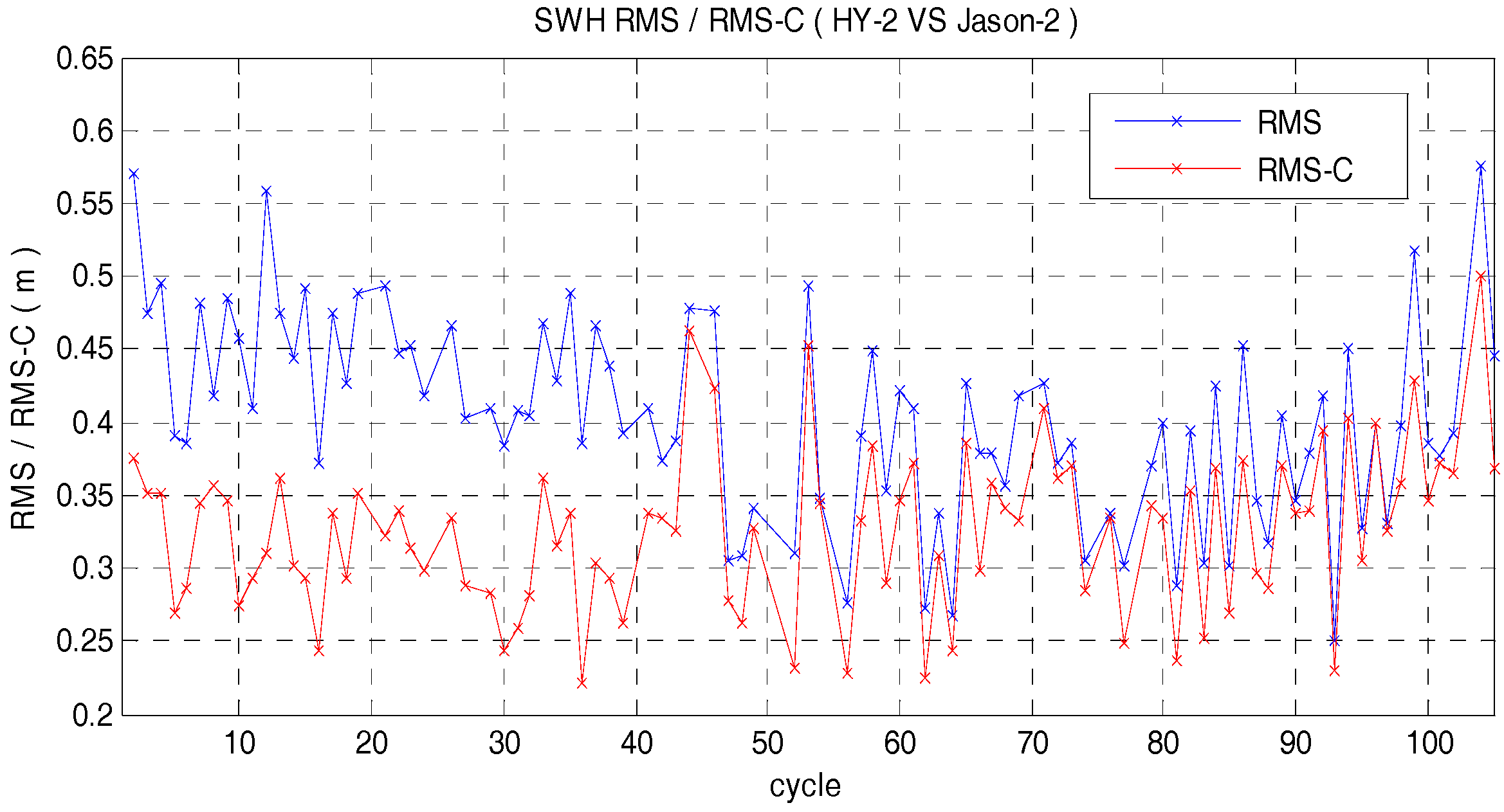
The accuracy of HY-2 SWH is shown in Figure 6, Figure 7 and Figure 8, and statistical results are given in Table 1, Line 3. Compared with Jason-2 SWH data, the mean value of differences is −0.21 m, with a 0.42 m RMS and a corrected RMS of 0.36 m. Using a linear regression fit, the linear regression formula was hs, J2 = 1.030 × hs, HY-2 + 0.1280, where hs, J2 is the Jason-2 SWH. The linear regression corrected HY-2 SWH against Jason-2 SWH is shown in Table 1, Line 5, and the RMS is reduced to 0.36 m.
4. Discussion
Using NDBC data and Jason-2 data, HY-2 IGDR SWH data were validated. Table 1 provides the statistical results for HY-2 SWH comparisons. As indicated in Table 1, the RMS was similar in the two comparisons, about 0.3~0.4 m; the two RMSs were similar, and the linear regression formula was also similar. Thus, validations of NDBC and Jason-2 comparisons with HY-2 have good consistency. The RMS of the Jason-1 SWH was 0.35 m when the NDBC SWH was used to validate Jason-1, and the RMS of Jason-2 SWH was 0.37 m at the Ocean Surface Topography Science Team 2008 meeting [17]. The HY-2 RMS was 0.33 m when validated by NDBC SWH, which is very similar to the accuracy of the Jason-1/2 SWH. Yang et al. used the NDBC to validate the HY-2 SWH data, and the correction formula was hs, NDBC = 1.0698 × hs, HY-2 + 0.1397 [7], which presents a slope similar to that of our ALT-A result: hs, NDBC = 1.071 × hs, HY-2 + 0.0700. The overall negative bias of HY-2 SWH has been shown to be about 0.2~0.3 m, and the RMS shown to be about 0.3~0.4 m compared with the NDBC SWH [12,13,14,15,16], which is similar to our work (Table 1).
Queffeulou has done long-term quality status validations with international operational altimeters, showing that the corrected ERS-1 RMS is 0.28 m, that the corrected ERS-2 RMS is 0.27 m, and that the corrected POSEIDON of T/P RMS is 0.25 m when compared with Buoy SWH [10]. The final report of Cross-Validation of ENVISATRA-2 Significant Wave Height, Sigma0 and Wind Speed shows that the RMS of the corrected ENVISAT RA-2 SWH is 0.32 m, and the RMS of Jason-1 is 0.27 m [20]. The RMS of corrected HY-2 data compared with NDBC data is 0.30 m (Table 1 Line 2), which indicates that the accuracy of HY-2 SWH is similar to that of the international operational altimeters, and the linear regression formula is useful in the correction of HY-2 SWH.
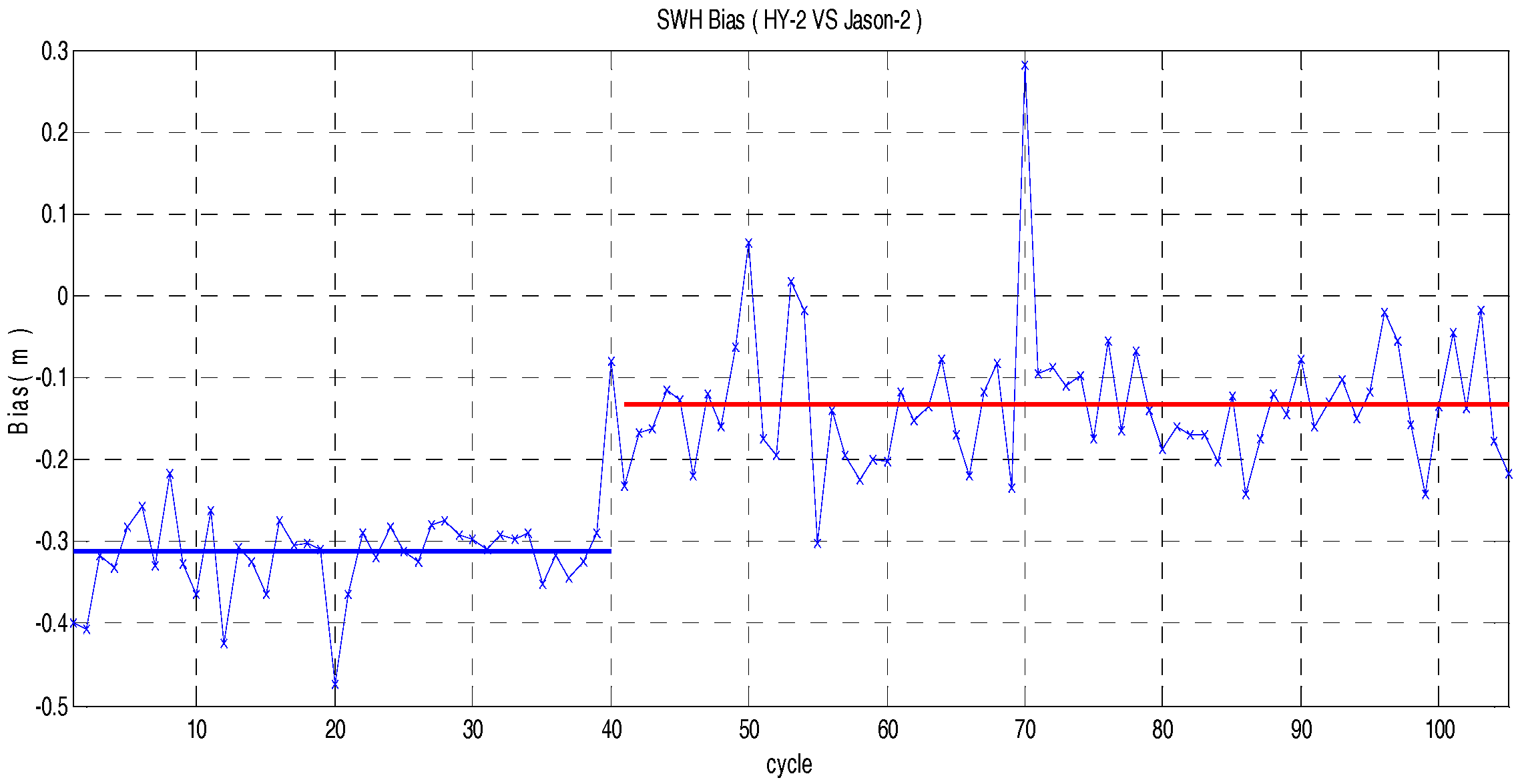
By comparing NDBC with Jason-2, it is obvious that the HY-2 SWH is lower than others in whole sea state situations (see Figure 4 and Figure 8). The bias of HY-2 SWH clearly jumps during Cycles 40 and 41 (see Figure 2 and Figure 6), which was caused by altimeter sensor switching from primary (ALT-A) to backup (ALT-B); the ALT-A and ALT-B have different accuracies and linear regression; the accuracy of ALT-A is lower than ALT-B, as shown in Table 1, Line 3, and Line 4, almost 0.10 m in RMS; but after the linear regression, the accuracy is almost the same.
4.1. HY-2 SWH Uncertainty Analysis
The uncertainty of HY-2 SWH was estimated by coincident NDBC SWH. The RMS between the HY-2 and the NDBC included the uncertainty in HY-2 measurements (∆HY2), the uncertainty in NDBC measurements (∆NDBC), and the uncertainty due to spatial and temporal decorrelation (∆S,∆T) [21].
Evidently, ∆S and ∆T will equal to 0 in the ideal case that the data from HY-2 and NDBC are totally coincident. Thus, Equation (1) can be rewritten as
where the term of RMS (HY2-NDBC) (0, 0) is the RMS when the measurements of HY-2 and NDBC are totally coincident.
In order to make an estimation of ∆HY2, it is necessary to obtain the value of RMS (HY2-NDBC) (0, 0). In this paper, the temporal window was set to less than 0.5 h. The spatial interval effect can be estimated by forming a data set of the SWH uncertainty as a function of different spatial intervals.
The buoy data used here is regarded as “truth”; that is to say, the error of buoy SWH is negligible. Therefore, the RMS (HY2-NDBC) (0, 0) can be treated as the error of HY-2 SWH.
Consequently, using the correction formula (as shown in Figure 9), the uncertainty of HY-2 SWH can be written as
The accuracy of HY-2 SWH is 0.17 ± 0.04 m, which evaluated the uncertainty after being corrected by NDBC measurements. Twelve synchronal experiments in South China Sea were launched to validate the accuracy of the HY-2 SWH from October to November in 2011. The position of the buoy was exactly at the HY-2 altimeter ground point [12]. The bias was 0.22 m with an RMS of 0.27 m. Using the linear regression formula hs, buoy = 1.11 × hs, HY-2 − 0.413, the RMS of HY-2 SWH was reduced to 0.17 m, which is the same as the uncertainty of the HY-2 SWH evaluated by NDBC.
4.2. The Error Spatial Variation
Using the Jason-2 SWH data, the spatial variation in the HY-2 SWH error was evaluated. In order to reduce the error caused by spatial distance, the distance between HY-2 and Jason-2 was fixed to less than 3.5 km. The error bar figure of whole sea states is shown in Figure 10.
The range of RMS value (the vertical lines in Figure 10) is from 0.2 to 0.3 m, with no significant variation in latitude. The average sea state varies with latitude as shown in Figure 10, and the lower sea state is in the equatorial ocean region.
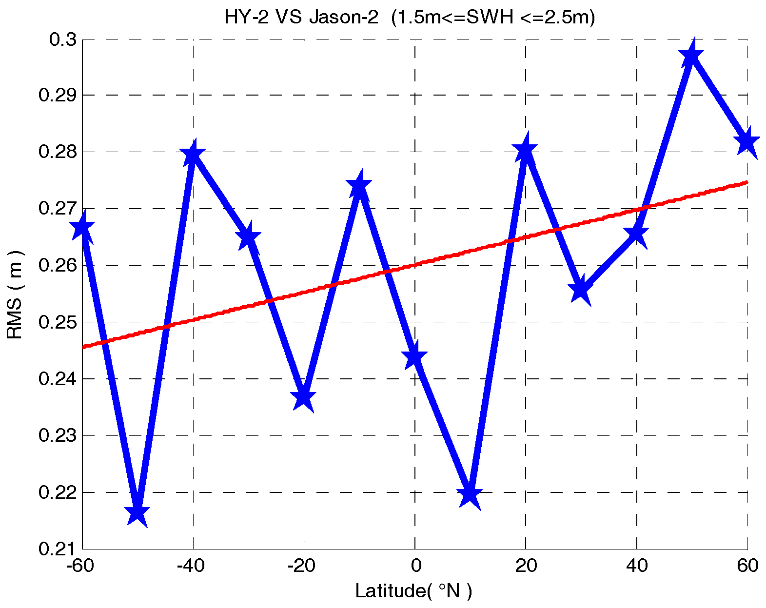
For analyzing the variation in the error bar with a latitude in the same sea state, the sea state in the middle wave (1.5 m <= SWH <= 2.5 m) was selected. The range of RMS values (the blue line in Figure 11) is from 0.2 to 0.3 m. In the middle wave sea state, the RMS value increases with the latitude from south to north, as shown in Figure 11.
5. Conclusions
Using the NDBC data and Jason-2 data, the accuracy of HY-2 SWH measurements was validated. The results show that the HY-2 SWH raw data have an accuracy similar to that of the international operational Jason-1/2 SWH data. Using a linear regression formula, the accuracy of the corrected HY-2 SWH is obviously improved, indicating the feasibility of using a linear regression formula to correct the HY-2 SWH. The value of HY-2 SWH is higher in lower sea state situations and lower in the whole sea situation.
Using error budget analysis, the accuracy of HY-2 SWH is 0.17 ± 0.04 m, which evaluated the uncertainty after being corrected by NDBC measurements. The accuracy of HY-2 SWH has no significant variation with latitude in whole sea states, but in the middle wave sea state, the RMS value of HY-2 SWH is increasing with the latitude from south to north.
Acknowledgments
The authors would like to thank a number of people for contributing to this work, including the NSOAS of State Oceanic Administration for providing HY-2 RA SWH products. The authors also thank USA NDBC and the AVISO for providing buoy data and Jason-2 GDR data, respectively. This work was funded by the National Key R&D Program of China (2016YFC1401003), the National Natural Science Foundation of China (41406204, 41501417 and 41506205) and the Marine Public Welfare Project of China (201305032-3).
Author Contributions
Chuntao Chen wrote the manuscript; Jianhua Zhu and Chuntao Chen devised and implemented the HY-2 SWH validation scheme; Mingsen Lin, Yili Zhao, He Wang and Jin Wang designed and analyzed the error budget. All authors contributed to the discussion and revision of the manuscript.
Conflicts of Interest
The authors declare no conflict of interest.
References
- Fang, M.Q. An East China Sea (ECS) Model with Multi-sensor Satellite Data Driving and Assimilation and Studies of Some Phenomena in the ECS. Ph.D. Thesis, Ocean University of China, Qingdao, China, 2003. [Google Scholar]
- Fu, L.L.; Cazenave, A. Satellite Altimetry and Earth Sciences. A Handbook of Techniques and Applications; Academic Press: Cambridge, MA, USA, 2001; pp. 407–435. [Google Scholar]
- Chen, C.T. Using Muti-Sensor Satellite Data to Study the Variability of Kuroshio. Ph.D. Thesis, Ocean University of China, Qingdao, China, 2010. [Google Scholar]
- Skandrani, C.; Lefevre, J.M.; Queffeulou, P. Impact of multi-satellite altimeter data assimilation on wave analysis and forecast. Mar. Geodesy 2004, 27, 511–533. [Google Scholar] [CrossRef]
- Abdalla, S.; Bidlot, J.R.; Janssen, P.A.E.M. Assimilation of ERS and ENVISAT wave data at ECMWF. In Proceedings of the ENVISAT ERS Symposium, Salzburg, Austria, 6–10 September 2004. [Google Scholar]
- Rusu, L.; Guedes, S.C. Impact of assimilating altimeter data on wave predictions in the western Iberian coast. Ocean Model. 2015, 96, 126–135. [Google Scholar] [CrossRef]
- Yang, J.S.; Xu, G.J.; Yin, L.B. Data fusion of significant wave height from HY-2A and other satellite altimeters. In Proceedings of the SPIE 8532, Remote Sensing of the Ocean, Sea Ice, Coastal Waters, and Large Water Regions, Edinburgh, UK, 19 October 2012. [Google Scholar]
- Robinson, M.C. ENVISAT Calibration and Validation Plan. Rev.02; Doc: PO-PL-ESA-GS-1092. 2000. Available online: https://earth.esa.int/support-docs/calval/CalVal.pdf (accessed on 1 May 2017).
- Yves, M.; Bruce, H. Jason-1 CAL VAL Plan; Ref: TP2-J0-PL-974-CN; 2 April 2001. Available online: ftp://podaac.jpl.nasa.gov/allData/jason1/L2/docs/calval4.0.pdf (accessed on 1 May 2017).
- Queffeulou, P. Long-term Quality Status of Wave Height and Wind Speed Measurements from Satellite Altimeters. In Proceedings of the Thirteenth International Offshore and Polar Engineering Conference, Honolulu, HI, USA, 25–30 May 2003. [Google Scholar]
- Queffeulou, P.; Bentamy, A.; Croizé-Fillon, D. Proceedings of the OSTST 2010 Meeting: Validation Status of a Global Altimeter Wind & Wave Data Base, Lisbon, Portugal, 18 October 2010; Available online: https://www.aviso.altimetry.fr/en/user-corner/science-teams/ostst-swt-science-team/ostst-2010-lisbon/ostst-2010-presentations.html (accessed on 1 May 2017).
- Chen, C.T.; Zhu, J.H.; Lin, M.S.; Zhao, Y.L.; Huang, X.Q.; Wang, H.; Zhang, Y.G.; Peng, H.L. The validation of the significant wave height product of HY-2 altimeter-primary results. Acta Oceanol. Sin. 2013, 32, 82–86. [Google Scholar] [CrossRef]
- Yang, J.; Xu, G.; Xu, Y.; Chen, X. Calibration of significant wave height from HY-2A satellite altimeter. In Proceedings of the Proc. SPIE 9221, Remote Sensing and Modeling of Ecosystems for Sustainability XI, San Diego, CA, USA, 17–21 August 2014; Volume 9221, p. 92210B. [Google Scholar]
- Ye, X.; Lin, M.; Xu, Y. Validation of Chinese HY-2 satelliteradar altimeter significant wave height. Acta Oceanol. Sin. 2015, 34, 60–67. [Google Scholar] [CrossRef]
- Liu, Q.; Babanin, A.V.; Guan, C.; Zieger, S.; Sun, J.; Jia, Y. Calibration and validation of HY-2 altimeter wave height. J. Atmos. Ocean. Technol. 2016, 33, 919–936. [Google Scholar] [CrossRef]
- Peng, H.; Lin, M. Calibration of HY-2A satellite significant wave heights with in situ observation. Acta Oceanol. Sin. 2016, 35, 79–83. [Google Scholar] [CrossRef]
- Wang, J.C.; Zhang, J.; Yang, J.G. The validation of HY-2 altimeter measurements of a significant wave height based on buoy data. Acta Oceanol. Sin. 2013, 32, 87–90. [Google Scholar] [CrossRef]
- Abdalla, S.; Janssen, P.; Bidlot, J. Jason-2 Wind and Wave Products: Monitoring, Validation and Assimilation, OSTST 2008 meeting. Mar. Geodesy 2010, 33, 239–255. [Google Scholar] [CrossRef]
- Frank, M. Expected Differences Between Buoy and Rader Altimeter Estimates of Wind Speed and Significant Wave Height and Their Implications on Buoy-Altimeter Comparisons. JGR 1988, 93, 2285–2302. [Google Scholar]
- Queffeulou, P. Cross-validation ENVISAT RA-2 Significant Wave Height, Sigma0 and Wind Speed. CCVT final report, France May 2003, IFREMER, BP, 70: 29280. Available online: https://www.researchgate.net/publication/268341138_Cross-validation_of_ENVISAT_RA-2_significant_wave_height_sigma0_and_wind_speed (accessed on 1 May 2017).
- Chen, G.; Xu, P.; Fang, C.Y. Numerical Simulation on the Choice of Space and Time Windows for Altimeter/Buoy Comparison of Significant Wave Height. In Proceedings of the 2000 IGARSS Geoscience and Remote Sensing Symposium, Honolulu, HI, USA, 24–28 July 2000. [Google Scholar]
Figure 1.
Map of collocated National Data Buoy Center (NDBC) buoys.
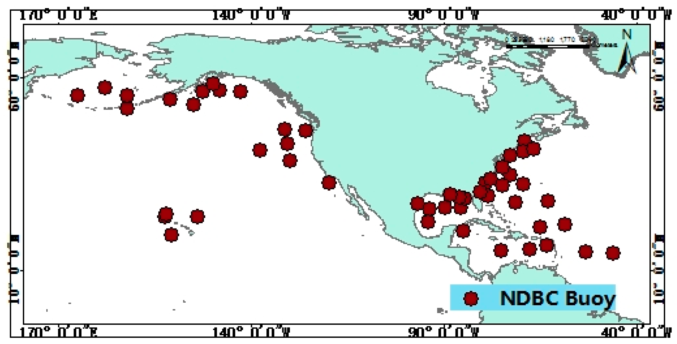
Figure 2.
The bias of HY-2 significant wave height (SWH) versus NDBC SWH.
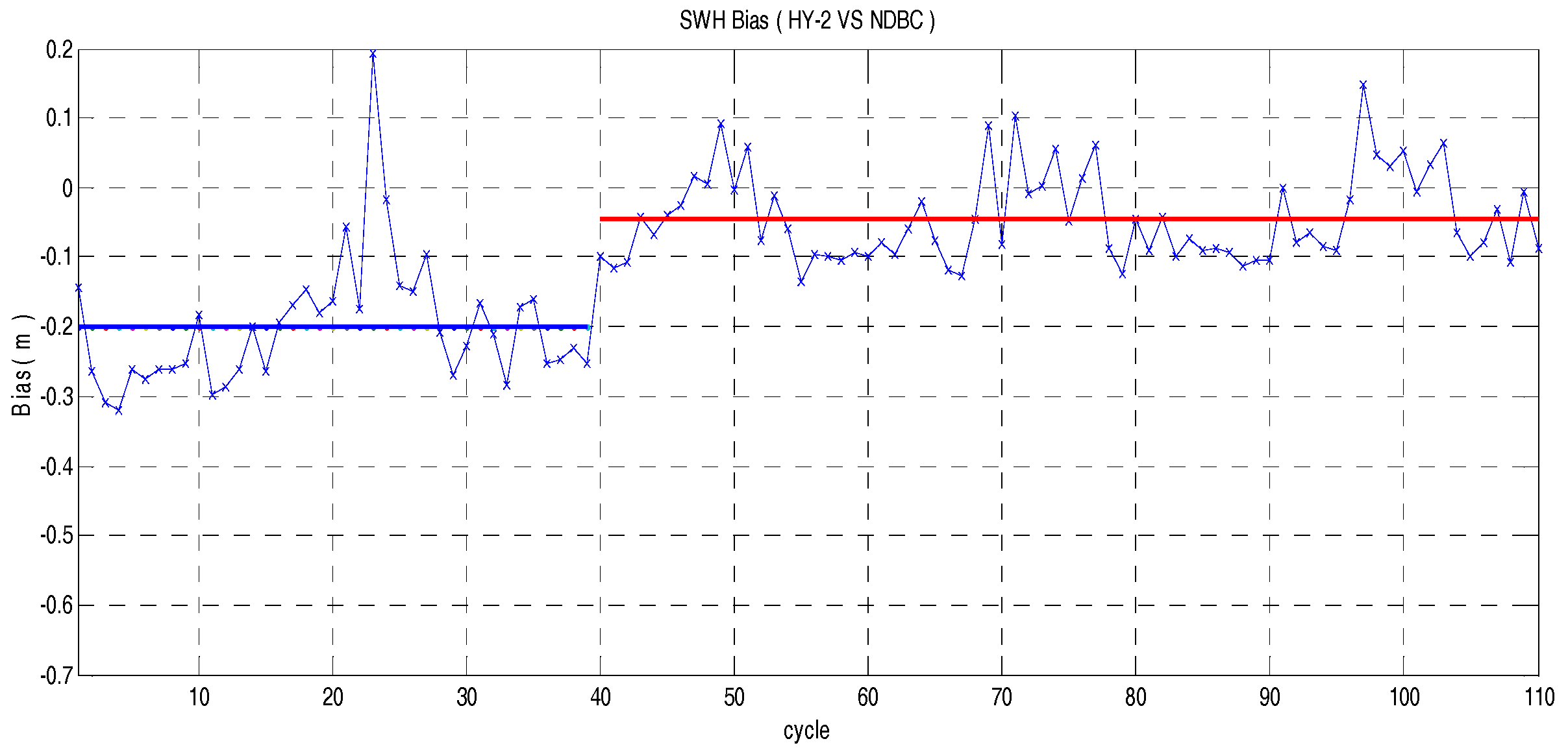
Figure 3.
The root mean square (RMS) and RMS-C of HY-2 SWH versus NDBC SWH. The red line is the RMS of HY-2 SWH versus NDBC SWH, and the blue line is the RMS of corrected HY-2 SWH versus NDBC SWH.
Figure 3.
The root mean square (RMS) and RMS-C of HY-2 SWH versus NDBC SWH. The red line is the RMS of HY-2 SWH versus NDBC SWH, and the blue line is the RMS of corrected HY-2 SWH versus NDBC SWH.
Figure 4.
Scatter plot of HY-2 SWH versus NDBC SWH.
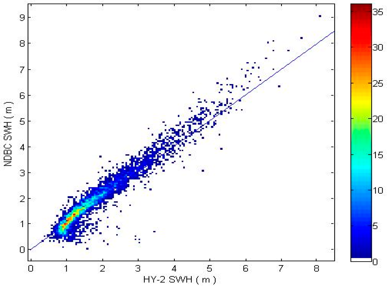
Figure 5.
Map of HY-2 versus Jason-2 crossing points.
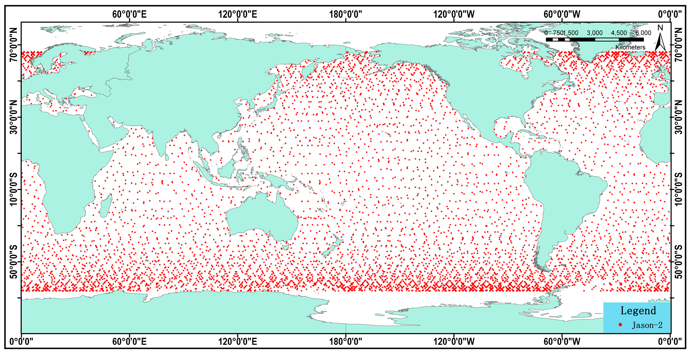
Figure 6.
The bias of HY-2 SWH versus Jason-2 SWH.

Figure 7.
The RMS and RMS-C of HY-2 SWH versus Jason-2 SWH.

Figure 8.
Scatter plot of HY-2 SWH versus Jason-2 SWH.

Figure 9.
The RMS variation with spatial distance between HY-2 and NDBC.
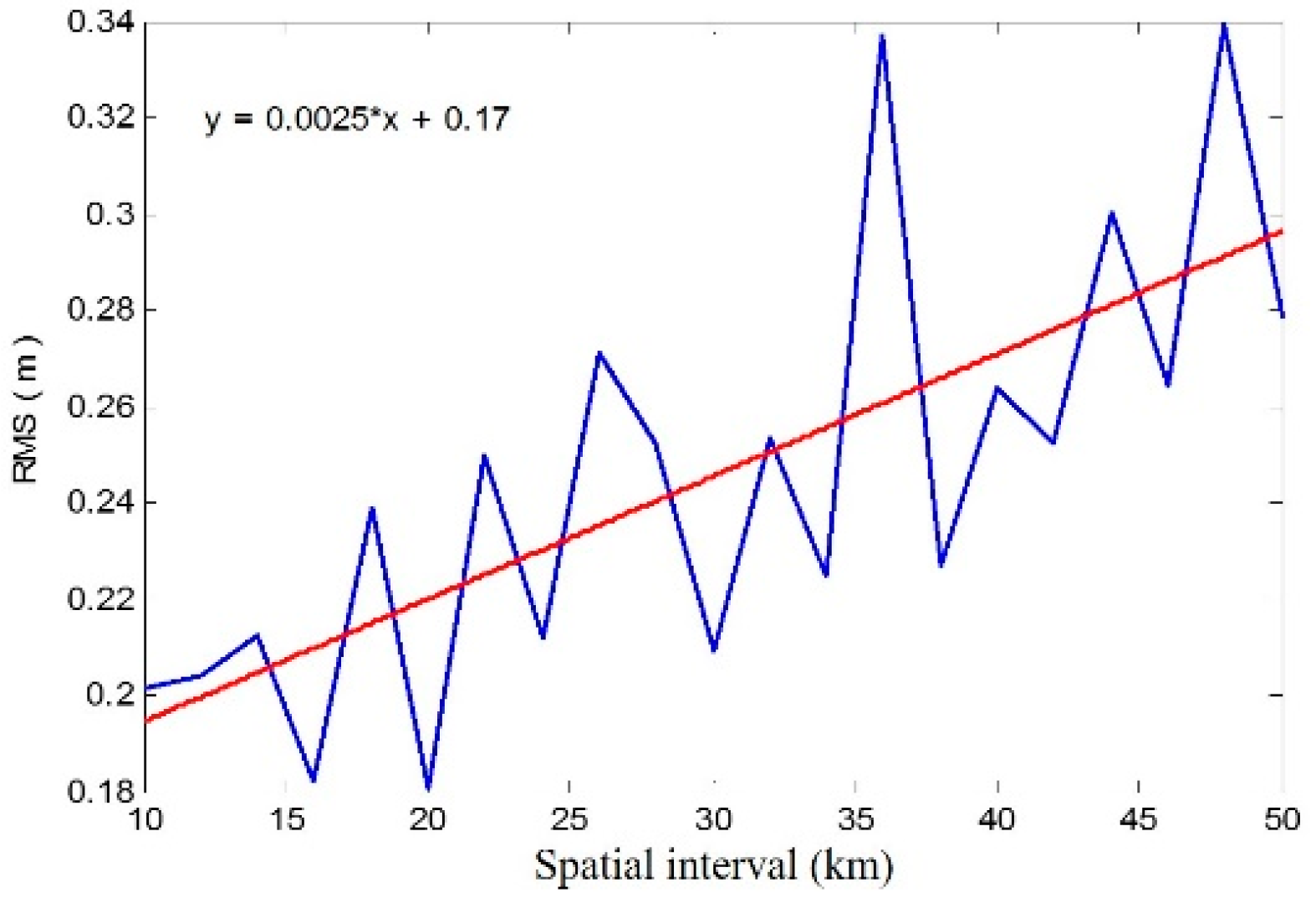
Figure 10.
The variation in the error bar with a latitude between HY-2 and Jason-2 in whole sea states. The curve indicates that the average value of Jason-2 SWH in the latitude ±5° range, and the vertical lines indicate the RMS values.
Figure 10.
The variation in the error bar with a latitude between HY-2 and Jason-2 in whole sea states. The curve indicates that the average value of Jason-2 SWH in the latitude ±5° range, and the vertical lines indicate the RMS values.
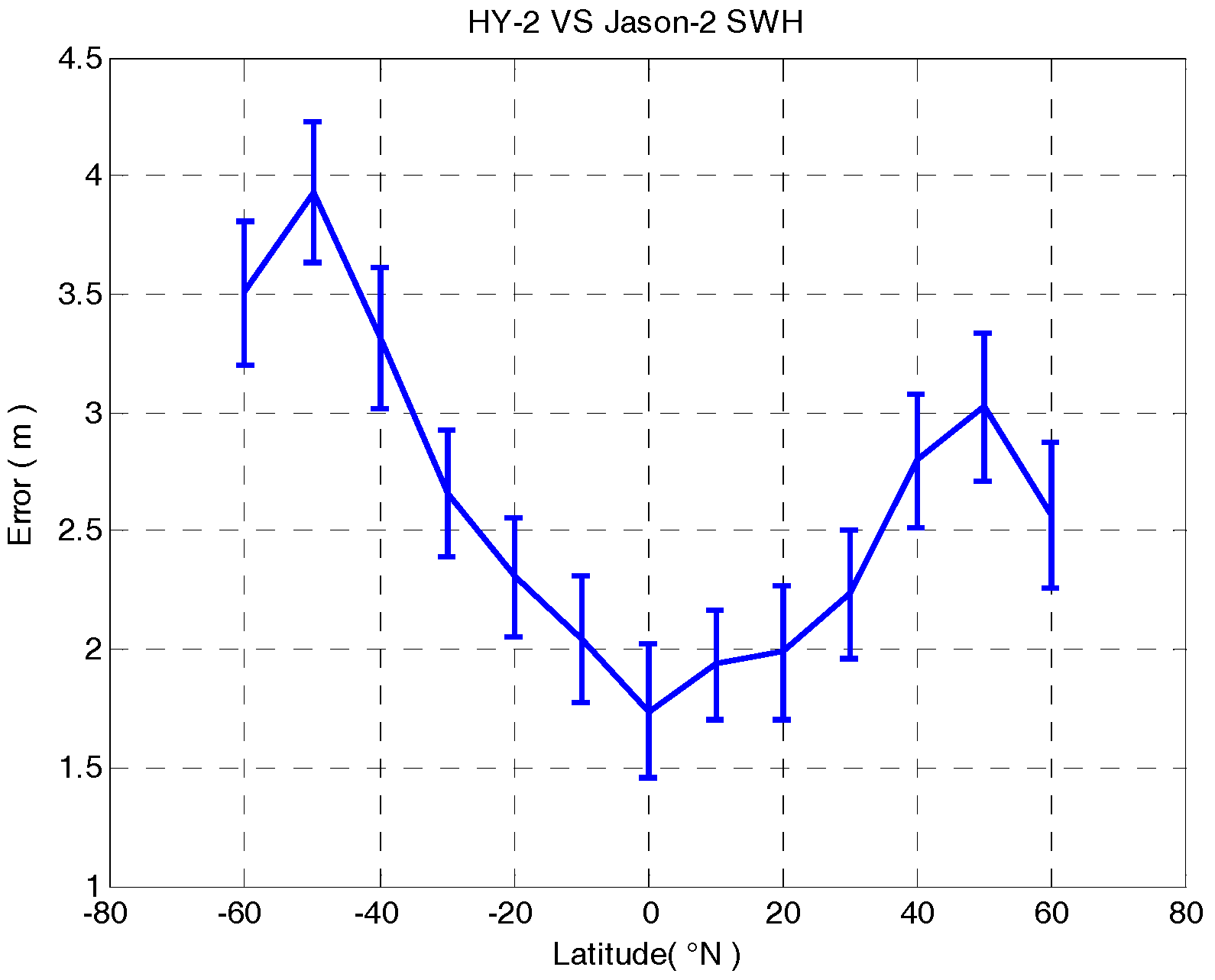
Figure 11.
The variation of error bar with latitude between HY-2 and Jason-2 in the middle wave (1.5 m <= SWH <= 2.5 m). The red line is a trend line.
Figure 11.
The variation of error bar with latitude between HY-2 and Jason-2 in the middle wave (1.5 m <= SWH <= 2.5 m). The red line is a trend line.


Table 1.
Statistical results for altimeter buoy SWH comparisons: bias, RMS, and RMS-C of differences between HY-2 SWH and others measurements, as well as linear regression slope and intercept.
Table 1.
Statistical results for altimeter buoy SWH comparisons: bias, RMS, and RMS-C of differences between HY-2 SWH and others measurements, as well as linear regression slope and intercept.
| Number | Bias (m) | RMS (m) | RMS-C (m) | Slope | Intercept | |
|---|---|---|---|---|---|---|
| NDBC | 4838 | −0.10 | 0.33 | 0.30 | 1.070 | −0.0278 |
| ALT-A | 1774 | −0.20 | 0.39 | 0.32 | 1.071 | 0.0700 |
| ALT-B | 3064 | −0.04 | 0.29 | 0.27 | 1.069 | −0.0817 |
| Jason-2 | 8714 | −0.21 | 0.42 | 0.36 | 1.030 | 0.1280 |
© 2017 by the authors. Licensee MDPI, Basel, Switzerland. This article is an open access article distributed under the terms and conditions of the Creative Commons Attribution (CC BY) license (http://creativecommons.org/licenses/by/4.0/).
Share and Cite
MDPI and ACS Style
Chen, C.; Zhu, J.; Lin, M.; Zhao, Y.; Wang, H.; Wang, J. Validation of the Significant Wave Height Product of HY-2 Altimeter. Remote Sens. 2017, 9, 1016. https://doi.org/10.3390/rs9101016
AMA Style
Chen C, Zhu J, Lin M, Zhao Y, Wang H, Wang J. Validation of the Significant Wave Height Product of HY-2 Altimeter. Remote Sensing. 2017; 9(10):1016. https://doi.org/10.3390/rs9101016
Chicago/Turabian StyleChen, Chuntao, Jianhua Zhu, Mingsen Lin, Yili Zhao, He Wang, and Jin Wang. 2017. "Validation of the Significant Wave Height Product of HY-2 Altimeter" Remote Sensing 9, no. 10: 1016. https://doi.org/10.3390/rs9101016
Note that from the first issue of 2016, this journal uses article numbers instead of page numbers. See further details here.