Quantifying and Reducing the DOA Estimation Error Resulting from Antenna Pattern Deviation for Direction-Finding HF Radar


The School of Electronic Information, Wuhan University, Wuhan 430072, China
*
Author to whom correspondence should be addressed.
Remote Sens. 2017, 9(12), 1285; https://doi.org/10.3390/rs9121285
Submission received: 16 October 2017
/
Revised: 4 December 2017
/
Accepted: 6 December 2017
/
Published: 11 December 2017
(This article belongs to the Special Issue Ocean Radar)
Abstract
:High-frequency (HF) radars are routinely used for remotely sensing ocean surface currents. However, the performance of the most widely used direction-finding HF radar is degraded due to the effect of the inevitable deviations of actual antenna pattern on the direction of arrival (DOA) estimation. In this paper, we quantify the DOA estimation error resulting from the deviation of the actual antenna pattern from the ideal one. Theoretical analysis and field experiment results suggest that the ratio of the deviations for the two loops dominates the DOA estimation error. Thus, eliminating the effect of the antenna pattern deviations on DOA estimation error is transformed into eliminating the effect of this ratio. From this, a calibration method based on the time-averaged local spatial coverage rate (TLSCR) is proposed to reduce the effect of the antenna pattern deviations on current extraction, which uses the ideal antenna pattern to estimate the DOA of the echoes. To validate this proposed calibration method, we assess the radar-derived radial velocities by comparing with in situ observations. The comparison results indicate that the proposed TLSCR calibration method can effectively reduce the DOA estimation error and improve the performance of the direction-finding HF radar in current observation.
1. Introduction
Shore-based high-frequency (HF) radars, working at a frequency between 3 MHz and 30 MHz, have now been widely used to remotely sense the coastal-ocean-surface current velocities [1]. These radars can observe current velocities out to a range of about 300 km offshore depending on the operating parameters of the radar system. Additionally, the current mapping results are provided in real time with a variety of temporal resolutions (normally around one hour) and spatial resolutions (from hundreds of meters to kilometers). These results are invaluable in many fields, including oceanographic and meteorological research [2,3,4], tsunami warning [5], search and rescue support [6], and monitoring of oil spills in real time [7].
There are two types of current-observing HF radar systems: direction-finding (e.g., the Coastal Ocean Dynamics Application Radar (CODAR; [8]) and Ocean State Measuring and Analyzing Radar, type S (OSMAR-S; [9])) and beam-forming (e.g., Wellen Radar (WERA; [10])). These two types of HF radar systems employ two distinct methods as well as two types of different antenna arrays to resolve the direction of arrival (DOA) of the sea echoes. The direction-finding radars adopt a small-aperture antenna consisting of a monopole and two orthogonal loops to form a quite broad beam for receiving the sea echoes [11]. The DOA of the sea echoes are determined by exploiting the directional properties of the compact antenna using the multiple signal classification (MUSIC) algorithm [12,13]. Beam-forming radars, using a distributed array of elements, electronically scan the ocean surface with a relatively narrow beam. The DOA of the sea echoes is identified by the delay and sum approach. This type of HF radar can achieve an excellent angular resolution to determine the bearing of the sea echoes. However, the preferred and more widely used HF radar system is the direction-finding HF radar because it uses a small-aperture antenna to accomplish surface current mapping, which leads to easy installation and maintenance.
Although many studies have validated the performance of the direction-finding radars in current observation by comparisons with in situ measurements [14,15,16,17], the calibration of the antenna pattern distortion and the channels’ gain/phase errors are still receiving significant attention due to the sensitivity of the compact antenna to its surroundings and the sensitivity of the MUSIC algorithm to the antenna pattern deviation. Some studies have suggested that using a measured antenna pattern to calibrate the antenna can improve the performance of direction-finding radar in measuring ocean surface currents [18,19,20]. To measure the actual antenna patterns, these studies carried out field measurements with an elaborately designed shipborne transponder moving along a pre-determined path. Obviously, these field measurements require extra equipment, leading to higher system cost. Carrying out these antenna pattern measuring experiments is also inconvenient due to the dependence on the weather and terrain conditions. Although Washburn et al. [21] have proposed a more simple pattern-measuring method based on an aerial drone, this method is also limited by the weather conditions and surrounding obstacles (severe weather, high buildings, and trees may cause hazards in performing this method). Fortunately, an automatic method for measuring the antenna pattern with ships’ echoes has been developed [22,23,24]. This automatic method needs almost no human intervention, but the angular coverage of the antenna pattern measured by this method may be limited depending on the orientation of the shipping lanes relative to the radar site [23]. In addition to these difficulties in measuring the actual antenna pattern, the measured antenna pattern often contains too much structure for the pointing algorithm to handle, resulting in persistent gaps with radial velocities crowding onto the gap boundaries for the retrieved radial current maps (see Figure 3 in [25] and Figure 6 in [15]). Although smoothing the measured antenna pattern can mitigate the gaps, this smoothing also leads to errors in DOA determination [26]. Therefore, using the measured antenna pattern to calibrate the antenna for direction-finding radar can only partially mitigate the accuracy reduction resulting from the deviation of the actual antenna pattern from the ideal one [27]. Furthermore, Atwater and Heron [28] suggested that the errors in radar-measured surface currents were insensitive to the measured and ideal antenna patterns. In addition, some other studies suggest that in some cases the current velocities extracted by the ideal antenna pattern show a better reliability than those extracted by the actual antenna pattern [26,29,30]. Therefore, using the ideal antenna pattern to retrieve the current mappings in direction-finding radar remains an indispensable technique, which is still widely used today.
However, in practice, using the ideal antenna pattern to retrieve the current mappings has to be faced with the DOA estimation error resulting from the actual antenna pattern deviation [31]. This DOA estimation error leads to the correctly determined radial velocities being placed into incorrect bearing sectors. However, so far, a quantitative relationship between the antenna pattern deviation and the DOA estimation error for the compact monopole-cross-loop antenna is absent. In this paper, we investigate the relationship between the antenna pattern deviation and the DOA estimation error, and present a detailed analytical derivation of the DOA estimation error stemming from the antenna pattern deviation. Theoretical analysis and field experiment results suggest that the relative deviation of the two loops dominates the DOA estimation error.
Moreover, to eliminate the DOA estimation error resulting from the antenna pattern deviation, we proposed a novel calibration method for extracting radial mappings using ideal antenna pattern. The proposed calibration method, called the time-averaged local spatial coverage rate (TLSCR) calibration method, is based on the quantitative analysis of the effect of the antenna pattern deviation on the DOA estimation error. To validate this calibration method, current-observing field experiments were carried out. Comparing the hourly averaged radial current velocities extracted by using ideal antenna pattern and involving the TLSCR calibration method with the buoy-recorded current velocities shows that the radar-derived current velocities agree well with buoy-recorded current velocities, with correlation coefficients being more than 0.96 and root-mean-square errors of about 10 cm/s. Additionally, the bearing offset is effectively reduced by implementing the TLSCR calibration method. Moreover, a comparison of the TLSCR calibration method with the only well-documented calibration method without any known sources [11] (hereinafter referred to as the conventional calibration method) has been carried out. Results suggest that the TLSCR calibration has a better performance than the conventional calibration method. In addition, some potential factors relating to the TLSCR calibration method have been discussed. These results demonstrate the reliability of the proposed TLSCR calibration method.
The paper is organized as follows. In the following section, we formulate the effect of the antenna pattern deviations on current observation for direction-finding radar. In Section 3, we present the quantitative relationship between the DOA estimation error and the antenna pattern deviations. In Section 4, we propose the TLSCR calibration method. To validate the quantitative relationship and the proposed calibration method, a field experiment has been carried out, and results are given in Section 5. Section 6 gives a discussion followed by a conclusion in Section 7.
2. Problem Formulation
Direction-finding radar uses a compact three-collocated antenna consisting of one monopole and two orthogonal loops (cosine loop and sine loop). These antennas have the properties of sharing a common phase path, but the gains are different from each other in any direction. Theoretically, the two orthogonal loops, respectively, have cosine and sine radiation patterns relative to the monopole, and the monopole gives an omnidirectional radiation pattern, which can be expressed as
where , , and are the ideal antenna patterns for the cosine loop, sine loop, and the monopole, respectively; is the look angle of the radar. This ideal antenna pattern is illustrated in Figure 1. The orientation of the cosine loop (0°, Figure 1) is usually called the normal direction.
However, the actual amplitude and phase patterns of the three elements always deviate from the ideal antenna pattern, due to the irregularity of the electromagnetic environment. Additionally, these deviations will always accompany the current extraction process, resulting in poor-quality ocean surface current mappings, unless they are intentionally calibrated. The amplitude and phase deviations, defined as the ratio of the actual antenna pattern to the ideal antenna pattern (the singular points for the directions leading to or is excluded), can be denoted by
where is the index of the three antenna elements; j is an imaginary unit. In fact, these amplitude and phase deviations in Equation (2) have included the antenna pattern distortion and the channels’ gain/phase errors, which are caused by the inconsistency among antenna elements, cables, and receivers (thus, hereinafter we refer to as amplitude and phase deviation or antenna pattern deviation in order to distinguish from the antenna pattern distortion). In addition, is a constant being equal to one because the antenna pattern of the monopole-cross-loop antenna is measured as the two loops relative to the monopole. Furthermore, so do the amplitude and phase deviations (i.e., ). Thus, the sample matrix, , for a sea echo S coming from the direction of at sampling instant t can be expressed as
where , , and are the output signals from the three elements of the antenna, and the superscript, T, denotes the transposition; is the deviation matrix of the amplitude and phase; is the ideal steering vector for the source coming from the direction of ; is the noise in the three antenna elements.
To determine the DOA of the signal by ideal antenna pattern, the approach of MUSIC first determines the noise subspace of the observations. Then, the signal bearing is found by projecting all the steering vectors onto that noise subspace [13]. The noise subspace estimation is typically achieved by carrying out an eigenvalue decomposition on the covariance matrix, , formed from the sample matrix. The covariance matrix can be estimated as , where N is the number of snapshots and H is the Hermitian transpose. Assuming that the noise is spatially white, the decomposition of the has the following form:
where is the signal eigenvalue and is the noise power; is the so-called signal subspace, and the orthogonal complement subspace spanned by is the noise subspace. The MUSIC algorithm tries to find the bearing that minimizes (maximizes) the projections of the steering vectors on the noise (signal) subspace, which can be expressed as the following MUSIC function:
If there is no amplitude or phase deviations for the monopole-cross-loop receiving antenna, and ignoring the effect of the noise (in practice, the signal-to-noise ratio of the selected Bragg lines is high enough, say more than 8 dB, resulting in a negligible effect of noise on DOA estimation; and just as the radial velocities comparisons in Section 5.2.4, the accuracy of the estimated velocities is independent of the range or independent of signal-to-noise ratio), the signal subspace must be spanned by the ideal steering vector of the incident signal (i.e., or ). Thus, is orthogonal to the noise subspace (), and Equation (5) achieves the minimum value at . However, for the deviated antenna pattern case, the signal subspace is spanned by the actual antenna pattern. Thus, we have
In this case, is no longer orthogonal to the noise subspace, , and DOA estimated by Equation (5) often deviates from . This deviation in DOA estimation will result in correctly determined radial velocities being placed into incorrect bearing sectors. It finally produces poor-quality current mappings. Although the bearing offset of the direction-finding HF radar in current mapping has long been attributed to the amplitude and phase deviations, the documented quantitative or analytical relationship between the antenna pattern deviations and the DOA estimation error is absent. In the next section, we will analyze the effect of the amplitude and phase deviations on the DOA estimation, and give an analytic relationship to quantify this effect. We will also propose a calibration method to eliminate this effect in Section 4.
3. Quantifying the DOA Estimation Error Resulting from Antenna Pattern Deviation
In this section, we present a detailed analytical derivation of the relationship between the DOA estimation error and the antenna pattern deviation. This relationship is key to understanding and eliminating the effect of the antenna pattern deviation on current mapping for direction-finding HF radar.
One thing that we are fairly convinced of is that the MUSIC function’s first-order derivative () is equal to zero at its minimum. Provided that the MUSIC function reaches its minimum value at , an expression for can be obtained via the first-order approximation of the Taylor expansion of . Following the approach in [32], expanding about the estimated DOA for a small error, we can write
Thus, the error of estimated DOA, , can be determined by
with positive indicating that the estimated DOA, , is displaced clockwise from the actual DOA (). Considering the effect of the amplitude and phase deviations on DOA estimation, the DOA estimation error stems from the error of actual signal subspace and the ideal manifold formed by the ideal antenna pattern. The actual signal subspace () is spanned by (Equation (6)). Thus, the MUSIC function (Equation (5)) can be rewritten as
Using Equations (1), (2), and (6) in Equation (9), we have
where ; denotes extracting real part. From Equation (10), we can easily obtain and . Thus, the Equation (8) can be rewritten as
This equation indeed suggests that the DOA estimation error is related to not only the amplitude and phase deviations [] but also the real DOA (). In other words, the same amplitude and phase deviations in different bearings will generate different levels of DOA estimation error for the signals coming from the corresponding bearings. In addition, if the condition of (i.e., and ) is satisfied, the numerator of Equation (11) will be equal to zero, which leads to the DOA estimation error, , reducing to zero.
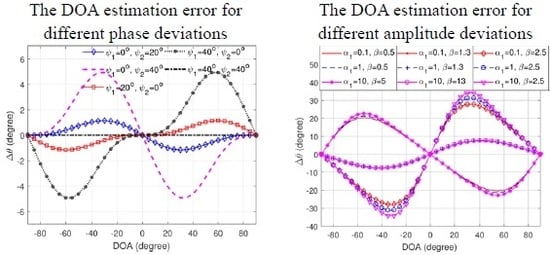
To demonstrate the relation between DOA estimation error and amplitude and phase deviation, we show the as a function of the incident signal’s DOA with different amplitude and phase deviations in Figure 2. We also force the amplitude and phase deviations to be constant (not varying with the bearing) for simplicity. Figure 2a suggests that the difference of phase deviations () affects the DOA estimation error. A 40-degree difference between the phase deviations results in at most 5 degrees DOA estimation error. Moreover, a 20-degree difference between the phase deviations is easy to achieve in real operation (see Appendix A). However, a two-time difference between the amplitude deviations () can lead to a DOA estimation error of over 20 degrees. Therefore, the presence of moderate phase deviations will have a limited impact on DOA estimation of the radial currents. The amplitude deviation has a much more significant influence on the DOA estimation. In addition, the DOA estimation error is an odd function as the DOA. Therefore, the estimated DOAs for signals coming from the different sides of normal direction are displaced with the opposite direction (for , if DOA > 0, then 0 or displaced clockwise, and if DOA < 0, then 0 or displaced counterclockwise; for , if DOA > 0, then 0 or displaced counterclockwise, and if DOA < 0, then 0 or displaced clockwise). This displacement will lead to the estimated DOAs moving toward the orientation of the cosine loop (0° and 180°, Figure 1) for the case of or toward the orientation of the sine loop (90° and 270°, Figure 1) for the case of . This displacement will affect the distribution pattern of the output radial velocities on the pre-determined range-bearing grid.
As a matter of fact, the phase deviations are easy to calibrate, and the typical distribution and the calibration method are presented in Appendix A. Therefore, the effect of the phase deviations in Equation (11) can be neglected after handling the phase deviations. Thus, turns into real numbers (i.e., ), and Equation (11) can be expressed as
Figure 2b shows the case of this equation. Now, setting
the quantitative relation between the DOA estimation error and the amplitude deviations is then re-expressed as
In fact, is insensitive to the value of , but quite sensitive to the value of . If the reserved parameter is , this insensitivity will be transferred to , definitely. Figure 3a shows the variation of DOA estimation error, , varying as a function of DOA with different combinations of and . For simplicity, we assume that and are constant and independent of bearing. As Figure 3a suggests, the spontaneous clustering of the curves based on the precisely demonstrates this insensitivity for and sensitivity for . For a given value of , plays a negligible role in on each bearing. Conversely, for a given value of , the values of vary rapidly for different . Therefore, is indeed insensitive to the value of but quite sensitive to the value of . This insensitivity of to is also verified by partial derivative in Appendix B. This insensitivity provides solid evidence to prove that the DOA estimation error is dominated by , which is the ratio of the amplitude deviations of the two loops or the relative amplitude deviations of the two loops. On the other hand, simulation results for the DOA estimation error under different antenna pattern deviations are shown in Figure 3b to verify the correctness of the quantitative relationship described in Equation (14). The simulation results are achieved by a Monte Carlo simulation of 500 independent runs with 20 snapshots for each trial, and the signal-to-noise ratio used in the simulation is 8 dB. Comparing Figure 3b with Figure 3a, we can clearly see that the simulation results are almost the same as the theoretical calculated results. Divergences for at the DOA near ±30° are owing to the approximation in Equation (7). This result suggests that the quantitative relationship is valid. In addition, this quantitative relationship and the result that the DOA estimation error is dominated by the relative deviation of the loop antennas (i.e., ) are truly innovating our understanding of the contribution of the antenna pattern deviation to current observation for direction-finding HF radar. We will carefully verify this result by the field experiment (see Section 5.2.5 and Section 5.2.6). Moreover, to demonstrate the application of this quantitative relationship, we propose a calibration method to eliminate the effect of the antenna pattern deviation on DOA estimation based on it.
4. Calibration Method for Reducing the DOA Estimation Error
4.1. Conventional Calibration Method
The only well-documented method for calibrating the monopole-cross-loop antenna without any auxiliary sources for ocean surface current observation was proposed by Lipa and Barrick [11]. We shall provide a brief introduction about this conventional method.
This conventional method only takes the channel errors into consideration, and the antenna pattern distortion is neglected. Thus, the amplitude and phase deviations are constant. Then, the signal model can be expressed as:
where () and () are the amplitude (phase) errors for cosine and sine loop, respectively. To calibrate the antenna, this conventional method estimates these four parameters based on the sea echo and then eliminates them by dividing by their estimators. For estimation of the amplitude deviations, a least-square method is adopted to fit the following equation:
and the value of and is calculated as the averaged phase deviations, which can be expressed as
where denotes computing the phase angles of complex number. In fact, Equation (16) is based on the ideal gain relationship between the monopole and the two loops (i.e., ). In this study, to implement this convention calibration method, we select the first-order Bragg peaks with signal-to-noise ratio (SNR) more than 15 dB in every one hour to estimate the amplitude and phase parameters (, , , and ). Thus, we adjust the value of gain and phase during the calibration procedure in every hour.
4.2. Proposed Calibration Method
Because the analysis of the relationship between the antenna pattern deviation and the DOA estimation error indicates that the DOA estimation error is controlled by and is nearly free from the effect of the value of , we will not calibrate the amplitude of the cosine loop. Additionally, we only calibrate the sine loop to yield . However, it is inadvisable in practice to strictly accomplish this objective due to the dependence of the amplitude deviations on the bearing. If we do this, the troubles encountered in calibrating the monopole-cross-loop antenna using the measured antenna pattern still exist. Thus, we must trade the DOA estimation performance off the feasibility. In this study, we calibrate the sine loop by multiplying the optimal correction factor, , to yield the value of being closest to 1 for the entire radar look angle space, which can be expressed as:
Obviously, the optimal correction factor in Equation (19) aims to yield close to 1 for the entire radar look angle space, but, for a specific bearing it may not be close to 1. If the measured antenna pattern is available, we can obtain immediately. Thus, the value of can be easily determined. However, we aim at estimating via an unknown source in this work because measuring the actual antenna pattern of the monopole-cross-loop antenna is a difficult task in practice.
Now, we give the recipe for estimating the optimal correction factor, . The value of represents the relative amplitude of to , and the displacement of the estimated DOA is now dependent on . If an improper correction factor is used, it will yield or in most of the bearings. The extremity that or for the entire radar look angle space is illustrated in Figure 2b and Figure 3a. Thus, if , the estimated DOAs will move toward the orientation of the sine loop. In contrast, if , the estimated DOAs will move toward the orientation of the cosine loop. Moreover, signals coming from 30° to 50° or −30° to −50° are most likely to be displaced due to in these bearings. Thus, these displacements will lead to the estimated radial current velocities crowding onto the orientation of the cosine loop (0° and 180°, Figure 1) or the sine loop (90° and 270°, Figure 1) but sparse in the bearing away from these orientations (30° to 50° or −30° to −50°). The optimal correction factor just eliminates these radial velocities crowding onto the orientation of the loops, so that the mapped radials will be uniformly distributed in a pre-determined radial grid. In other words, the radials will be distributed in as many direction cells as possible for all range cells. The valid estimator of the radials in the directions being away from the two loops orientations will reach its maximum. Therefore, a local area (LA) with an angle size of 40 degrees (motivations for these choices are given in Section 6.2) centered in the direction where the antenna patterns of the two loops intersect (i.e., 45°, 135°, 225°, and 315° in Figure 1) is chosen to estimate (an example for the selected LA is shown in Figure 4). The optimal correction factor should lead to the radial velocities mapped in this area being as many as possible. Thus, Equation (19) can be equivalent to
where represents an average over time (this time length is four days and the motivations for its value are presented in Section 6.2); is the number of sectors returning valid radial current solutions within the selected 40-degree area (or within LA); M is the total number of the pre-determined sectors in the LA. , defined in Equation (20), is referred to as the time-averaged local spatial coverage rate (TLSCR). Thus, we call this method for estimating to calibrate the compact antenna the TLSCR calibration method. To estimate the optimal correction factor, , from Equation (20), we search the maximum value of for varying in the range of 0.1 to 2.5 with an interval of 0.1. The motivation of this search method is that the hardware structure of the cosine loop is the same as that of the sine loop, resulting in having a limited value and our experience of using this method finds is always limited to the range of 0.4 to 2.5.
5. Field Experiment and Results
To verify the reliability of the TLSCR calibration method for calibrating the monopole-cross-loop antenna for direction-finding radar systems, we carried out a field experiment for current observation and used this calibration method to calibrate the antenna in the current extraction process. We demonstrate the reliability of the TLSCR calibration method by assessing the accuracy of the retrieved radial current velocities. Moreover, to show the improvement of the current mappings extracted by the proposed calibration method, we also evaluate the radial velocities retrieved by the conventional calibration method. Certainly, the radial mappings extracted by both the proposed and conventional calibration methods use the MUSIC algorithm to estimate the DOA of the sea echoes. Then, to give more solid evidence to validate the reliability of the TLSCR calibration, a testing case—another current-observation experiment—is provided. In addition, to validate the theory-deduced result that the DOA estimation error is dominated by the relative amplitude deviations for the two loops, we perform the current extraction procedure again with an extra manipulation; that is, multiplying a constant factor on the sea echoes received by the two loops after achieving the TLSCR calibration method. In fact, this extra manipulation is equivalent to adjusting the values of and , but yields being the same as the normal TLSCR calibration (non-execution of the extra manipulation). Thus, if the claim that the DOA estimation error is dominated by the relative amplitude deviations for the two loops is true, the radial velocities retrieved by involving the extra manipulation will agree well with the radial velocities retrieved by the normal TLSCR calibration. In fact, the reliability of the proposed TLSCR calibration method is solid evidence for proving the result that the DOA estimation error is demonstrated by the relative deviations of the two loops because the calibration method is just based on this result.
5.1. Field Experiment
The experiment was carried out in November 2015. In this field experiment, an HF radar system named OSMAR-S was installed in Fujian province, China, to observe the sea state of the Chinese East Sea. A geographic map of this experiment is shown in Figure 4, and the ideal antenna pattern is superposed on the map. The red solid dot represents the location of the radar site (DongShan (DOSH), 23°39.45′N, 117°29.23′E). The blue pentagram indicates the location of a buoy, which is about 75 km off the radar site. The bearing of this buoy to the radar origin is 48° (measured as clockwise to the normal direction, and hereinafter all the bearings have been measured in this way). This buoy was equipped with an acoustic Doppler current profiler (ADCP), which provided current velocities every 10 min with a velocity resolution of 4 cm/s. The buoy-recorded current velocities were used for checking the results of radar-derived radial velocities to validate the TLSCR calibration method.
The OSMAR-S developed by Wuhan University, China, is a direction-finding HFR system which adopts a compact cross-loop-monopole antenna for receiving the sea echoes. Similar to the CODAR and WERA HF radar systems, the OSMAR-S also contributes to the advancement of the HF radar community. The OSMAR-S uses a linear frequency-modulated interrupted continuous waveform in operation. During the experiment, the radar worked at a frequency of 13 MHz, with a bandwidth of 60 kHz, yielding a range resolution of 2.5 km. The maximum detection range was 120 km. Samples for each range cell were collected at an interval of 0.38 s. A 512-point fast Fourier transform was then performed to yield a coherent integration time of about 200 s, corresponding to a current velocity resolution of approximately 5.5 cm/s. The nominal direction resolution was set to 3 degrees in the direction-finding procedure.
5.2. Results
To validate the proposed calibration method, we extracted radial current mappings for every value of (ranging from 0.1 to 2.5 with an interval of 0.1). Then, we checked the relation between the spatial distribution of the temporal rate and . The temporal rate was calculated for each radial sector as the number of the radial mappings with a valid radial velocity estimator for the current sector divided by the total number of radial mappings. The TLSCRs for the two LAs (F1 and F2) were used to determine . The radial current velocities extracted in the case of calibrating the antenna using are compared with the buoy-recorded current velocities. Moreover, the radial currents extracted using the calibration method proposed by Lipa and Barrick [11] are shown as a contrast. Then, we present a testing case and we analyze the bearing offset for the above-mentioned field experiment and testing case. Finally, we validate the result that the DOA estimation error is dominated by the relative deviations of the two loops.
5.2.1. Spatial Distribution of Temporal Rate
The spatial distribution of the temporal rate—which is calculated for every radial sector as the number of the radial mappings with a valid radial velocity estimator for the current sector divided by the total number of radial mappings—for different correction factors are shown in Figure 5. The distributions of the temporal rate in Figure 5a–i are computed for the correction factor () varying from 0.1 to 2.4 with an interval of 0.3. Figure 5 indeed confirms that—just as inferred in Section 4.2— can significantly affect the spatial distribution of valid radial velocity solutions. From this figure, we can clearly see that the correction factor with a small value (e.g., ) leads to the radials crowding onto the edge of the detecting area, and a large value (e.g., ) results in the radials crowding onto the bearing near perpendicular to the coastline. In fact, these crowding regions are the orientation of the antenna pattern of the two loops (Figure 4). This crowding results in sparse radial velocity estimators in the two LAs, which are away from the orientations of the two loops, indicating a non-optimal value of . Additionally, as Equation (20) presents, the optimal value of the correction factor, , should lead to the mapped radials being uniformly distributed, and the valid estimators of the radials in the two LAs should achieve its maximum.
5.2.2. Time-Averaged Local Spatial Coverage Rate (TLSCR)
Figure 6 shows the TLSCR calculated within F1 and F2 (Figure 4) with varying values of the correction factor. The radial current mappings used to calculate these TLSCRs cover four days, from November 8th to November 11th. As indicated in this figure, the TLSCRs for both F1 and F2 increase at first then decrease with increasing values of . The black vertical line in the figure indicates the correction factor yielding a maximum of the TLSCR. As Figure 6 suggests, the value of the correction factor yielding a maximum value of TLSCR for F1 and F2 are the same. This figure definitely suggests that the value of the optimal correction factor should be 0.5 for DOSH and the optimal correction factor can be estimated from either F1 or F2.
5.2.3. Radial Velocity Comparison
To evaluate the validity of this estimated optimal correction factor, the reliability of the radial current mappings extracted in the case of calibrating the antenna with the correction factor of 0.5 is evaluated. We compare the radar-derived radial velocity time series with the buoy-derived radial current velocities at the buoy location. As a contrast, the radial current velocities extracted by calibrating the antenna using the conventional method are also compared with the buoy-derived radial velocities. Figure 7 shows the radar-derived radial velocity time series and those recorded by the buoy. The correction coefficient (r) and root-mean-square error (rmse) are displayed in the top of each panel. The comparisons in Figure 7a suggest that the radial currents extracted in the case of using the TLSCR calibration method are very accurate with a correlation coefficient of 0.96 and an rmse value of 9.67 cm/s (the radial velocities retrieved without any calibration processing have not been presented here because the radar–buoy comparison results for this case are implied in Figure 17). Therefore, the proposed calibration method is reliable. On the other hand, the conventional calibration method yields a correlation coefficient of 0.95 and an rmse value of 14.87 cm/s (Figure 7b). This result indicates that the proposed calibration method has a much better performance than the conventional method. The reason for the proposed calibration method having better performance than the conventional method is that the proposed calibration takes the antenna pattern deviations into consideration and the conventional method does not consider the antenna pattern deviations.
5.2.4. A Testing Case
Another current observation experiment using the OSMAR-S radar system was carried out in February, 2013. The geographic map of this experiment is shown in Figure 8 with the ideal antenna pattern superposed on it. This figure indicates that the antenna configuration in this experiment was greatly different from the DOSH. Because of the antenna configuration, there is only one local area (LA) included in the radar detection area. Two buoys of the same type as DOSH were deployed within the radar’s detection area. The ranges for the two buoys to the radar origin were 42 km for buoy A and 85 km for buoy B. The experiment lasted for a month, which is fairly long relative to the DOSH experiment. Long-term observation included more extreme environmental conditions (interference and sea state). Thus, this experiment provides a better chance to sufficiently validate the TLSCR calibration method.
We performed the proposed calibration method to retrieve the radial current mappings for this experiment. Then, the radial current velocities at the buoys’ location were compared with the buoy-derived radial current velocities. From the selected LA, the optimal correction factor derived from the radar data collected during the first 4 days—from 1 February to 4 February—is equal to 1.3. This optimal correction factor was used to calibrate the entire one-month data set. The radial current velocities extracted at the buoy locations are shown in Figure 9. The correlation coefficient (r) and root-mean-square error (rmse) are also displayed in this figure. The radar–buoy comparison results show that the correlation coefficients are 0.90 at buoy A and 0.94 at buoy B, and the rmse values are 11.44 cm/s and 9.00 cm/s for buoy A and buoy B, respectively. In addition, the comparisons between the radar-sensed radial velocities extracted by conventional calibration method with those recorded by the buoys indicate comparable correlation coefficients, but obvious degradation for rmse values (Figure 10 vs. Figure 9). These results suggest that the radial currents retrieved by the proposed calibration method are highly credible. Additionally, the difference of the antenna configuration had no effect on the calibration method. The only matter for the antenna configuration is that at least one LA should be guaranteed within the radar detection area. This criterion is generally likely to be met because the look angle of the radar is usually larger than the angle size of LA. Moreover, using the optimal correction factor estimated in the first four days to calibrate the antenna for the long term is still very effective. These results demonstrate the generalizability of the TLSCR calibration method.
5.2.5. Bearing Offset and Its Consistency with the Quantitative Relationship Described in Section 3
The bearing offset is an important indicator for evaluating the performance of HF radar, and therefore for validating the reliability of the proposed calibration method. Thus, we analyzed the bearing offset for the radial velocities extracted with no calibration and with the proposed calibration method. Then, we analysed the change of the bearing offset after performing the proposed TLSCR calibration method. Moreover, we also show the consistency of this change with the quantitative relationship between the antenna pattern deviation and the bearing offset (Equation (14)).
The bearing offset is defined as the bearing difference between the estimated bearing of the radial current velocities and the real bearing of these radials. The presence of the bearing offset leads to the radar sector that has the best matching current velocities in comparison with the current velocities recorded by in situ instruments deviating from the radar sector lying directly over the in situ instrument. Following the approach proposed by Emery et al. [14], the bearing offset, , can be quantified as , where is the bearing of the buoy and is the bearing to the sector with maximum correlation coefficient, with positive indicating that the sector showing maximum correlation coefficient is displaced clockwise from the buoy. Similarly, the root-mean-square error (rmse) can also be used to indicate the current mapping bearing offset ().
The results of bearing offset estimation are provided for all DOSH–buoy and SHanLIao (SHLI)–buoy pairs in Figure 11. The correlation coefficient and rmse are shown for each radar–buoy pair as a function of bearing in the range cell corresponding to the buoys’ location, with vertical lines indicating the bearing of the sector showing minimum rmse value (red line marked with stars), and the bearing of the buoy (thick black line). The bearing offsets are hence represented as the differences between these pairs of vertical lines. On the other hand, because the calculated correlation coefficients varying as a function of bearing have a flat peak, it may lead to relatively large errors of the estimated bearing offset if we estimate the bearing offset based on the correlation coefficient. Conversely, the rmse values varying with bearing have relatively narrow peak. As Figure 11b,e show, the correlation coefficient is almost constant with bearing in 50° to 100°. However, the rmse varies distinctly in this bearing range. In fact, the rmse indicates the difference between two variates and the correlation coefficient describes the consistent proportional increases or decreases about the two variates. Thus, if the current vector is parallel to the shore, the correlation coefficient between the buoy-derived radial velocities and the radar-derived radial velocities must be constant with bearings, so the correlation coefficient fails to reflect the bearing offset. Furthermore, in this study, the vector current profile may be locally parallel to the shore, so that the correlation coefficient is almost constant in a large bearing range. Thus, we adopt the rmse to estimate the bearing offset in this study. As Figure 11 suggests, the bearing offset (the absolute value of ) decreased for all the radar–buoy pairs comparisons after performing the proposed TLSCR calibration method. In addition, the bearing offset is not uniform over bearings because the bearing offset results from the antenna pattern deviation and the antenna pattern deviation is bearing dependent. Specifically, the TLSCR calibration method completely eliminated the bearing offset at the buoy direction in the DOSH site. For SHLI, the proposed calibration method produced lesser bearing offsets at both buoys A and B. These results indeed indicate that the proposed TLSCR calibration can effectively improve the performance of the direction-finding HF radar in ocean current observation.
In fact, the decrease of the bearing offset after performing the TLSCR calibration is consistent with the quantitative relationship between the antenna pattern deviation and the DOA estimation error. First, the bearing offset of the DOSH site at the buoy bearing is zero for the calibrated case (Figure 11d); that is, the TLSCR calibration produces the ratio of the two-loop amplitude deviations (denoted by ) being equal to 1. Thus, for the uncalibrated case, the ratio of the amplitude deviations, , must be equal to . Then, using , , and (according to Figure 3a, the value of has nearly no effect on the DOA estimation error) in Equation (14), we can obtain the theoretical bearing offset of the uncalibrated case for DOSH–buoy comparison. As summarized in the first row of Table 1, the theoretical bearing offset () is 20.71°, which is very close to the bearing offset () derived from the rmse profile. For the SHLI–buoy comparison, the bearing offset of the calibrated case is not equal to zero. We must use bearing offset (), , and in Equation (14) to solve . Then, for the uncalibrated case, the ratio of the amplitude deviations, , can be calculated as /. Using this approach, we obtained the values of as 0.63 and 1.12 at the bearings of buoy A and B. That is to say, after performing the TLSCR calibration for SHLI, the ratios of the amplitude deviations of the two loops are 0.63 and 1.12 at the bearing of buoys A and B, respectively. Thus, we can obtain that those ratios for the uncalibrated case are 0.63/1.3 = 0.48 and 1.12/1.3 = 0.86, respectively. Then, using these ratios and the bearings of these buoys in Equation (14), we can obtain the theoretical DOA estimation error for the uncalibrated case at the buoys’ bearing. As Table 1 describes, the results of the theoretical DOA estimation error () are very close to the bearing offset estimated based on the rmse profile for the uncalibrated case (). These results suggest that if we know the DOA estimation error for a certain bearing, we can know the relative deviation of the two loops, and vice versa. They also suggest that the quantitative relationship between the antenna pattern and DOA estimation error presented in this study is credible.
5.2.6. Validating the Conclusion That the DOA Estimation Error Is Dominated by the Relative Amplitude Deviations of the Two Loops
In this section, we examine the theoretical conclusion that the DOA estimation error is dominated by the ratio of the amplitude deviations of the two loops or the relative deviations of the two loops. To achieve this goal, we extract the current mappings again with an extract manipulation after completing the TLSCR calibration. This extra manipulation is that we multiply the same constant factor on the sea echoes in the two loops, which can result in the actual steering vector, , being transformed into , where and is the constant factor; is the the deviation matrix after performing the TLSCR calibration. Thus, this extra manipulation is equivalent to amplifying or diminishing the amplitude deviations of the two loops with the same number of times. In other words, this extra manipulation adjusts the values of and but keeps the same as the normal TLSCR calibration case (which does not involve the extra manipulation or which is equivalent to ). Then, we assess the accuracy of the current velocities and also assess the bearing offset for the radial mappings extracted by involving the extra manipulation.
In this study, the values of the constant factor () used in the extra manipulation are 0.2 and 20. Certainly, using other values of the constant factor must yield the same results as the results demonstrated in this section. For DOSH, the current velocities at the buoy location extracted involving this extra manipulation are shown in Figure 12. The radar–buoy comparison result for is shown in Figure 12a. The correlation coefficient and rmse are almost the same as the results displayed in Figure 7a. A similar comparison result is also illustrated in Figure 12b for . Moreover, the radar–buoy comparisons for SHLI at both buoys A and B also indicate the same result (Figure 13 and Figure 14). Although the rmse values for the cases of different values of have changes, these changes are very small and less than the current resolution of the radar system (5.5 cm/s). Thus, these results indicate that the accuracy of the radial velocities is dominated by the relative amplitude deviation of the two loops. On the other hand, we also examine the bearing offset for the cases of and . Figure 15 shows the rmse values varying with the bearing for the three radar–buoy pairs under different values of . We have not calculated the bearing offset directly because the rmse profiles for different values of are almost the same, which provides enough evidence to verify that there is almost no difference for the bearing offset in the cases of different . Thus, these results provide solid evidence to validate that the DOA estimation error is dominated by the ratio of the amplitude deviations of the two loops.
6. Discussion
6.1. Interpretation of the Fact That the Same Deviation in the Two Loops Will Not Lead to DOA Estimation Error
In this study, an analytical relationship between DOA estimation error and antenna pattern deviation has been presented (Equation (14)). From this analytical relationship, we conclude that the DOA estimation error is dominated by the relative deviations of the two loops, and the same deviation in the two loops will not lead to DOA estimation error. Now, we interpret this conclusion in another way. Provided that the deviations of the amplitude for the two loops are the same, the actual antenna pattern can be expressed as:
where is the amplitude deviation. For a signal coming from the direction of , the actual steering vector of this signal can be expressed as:
Then, we obtained the estimated DOA, , using the ideal antenna pattern and MUSIC algorithm. The DOA estimated in this way indicates that is the most similar steering vector to in terms of the entire look angle space. In fact, the similarity can be quantified by the Euclidean distance, , between the actual steering vector, , and the ideal-pattern-formed steering vector, . Thus, estimating the DOA is to minimize the Euclidean distance; that is,
In addition, the Euclidean distance is
From Equations (23) and (24), we can infer that . In other words, for the entire look angle space, is the most similar vector to . Namely, in the MUSIC algorithm, the value of this deviation (the value of ) will only affect the amplitude of the MUSIC function but not affect the position where MUSIC reaches its minimum value. Thus, the same deviation in the two loops cannot result in DOA estimation error.
6.2. Sensitivity Testing of the TLSCR Calibration Method
In Section 4.2, we have proposed a method to calibrate the antenna for a direction-finding radar system. The experimental results indicate that this method can effectively calibrate the antenna. Now, we examine the effect of the two parameters (the size of selected LA and time length for averaging in calculating TLSCR) in determining the optimal value of the correction factor.
The TLSCR calibration method is tested for different value combinations of the two parameters: the angle size of the LA varying from 10° to 60° and the time length, for averaging, varying from 0.5 day to five days. We adopt the variance to quantify the sensitivity of the estimated optimal correction factor () to these two parameters. The variance of the estimated , for different combinations of these two parameters, is shown in Figure 16. As made evident in this figure, for a given value of the angle size, the variance decreases with increasing time length. However, in practical application, a small value of time length is preferred due to the computing efficiency. In fact, the time length controls how much radial current mappings are used to calculate . In reality, a long time for estimating can effectively eliminate the effects of the interference (radio-frequency interference and ionospheric disturbance) and the actual sea state on determining the optimal correction factor. Therefore, the time length should last for a few days. On the other hand, for a given value of time length, the variance decreases with increasing angle size. However, for angle size increasing from 20° to 60°, the variance decreases very slowly for any given time length. In real application, a small angle size is also preferred. This is because the radar detection area is limited by the coastline and a smaller size area, centered at the direction where the antenna pattern of the two loops intersect, is easy to achieve within the radar detection area. Thus, the slow decrease of the variance for angle size increasing from 20° to 60° suggests that the choice of the angle size is pretty flexible; that is, a value of 20 degrees or 60 degrees for the angle size produces almost the same result. Therefore, angle size being 40° and time length being four days are suitable. Furthermore, the variance is very small even for angle size being 10 degrees and time length being 0.5 day. This small level of variance indicates that the TLSCR method is robust.
6.3. Interpretation of the Optimal Correction Factor
In this study, we only used a constant factor—the optimal correction factor—to calibrate the monopole-cross-loop antenna. Experiment results suggest that using the ideal antenna pattern and involving the proposed calibration method can achieve reliable performance for direction-finding HF radar. However, in practice, the antenna pattern of the collocated, three-element antenna is always distorted owing to the irregular electromagnetic environment. Thus, we must note that this optimal correction factor yields the minimum DOA estimation error for echoes homogeneously coming from the sea surface; that is, the echoes coming from each sector are equal-possibility or the echoes are not coming from a specific bearing scope. Furthermore, this optimal correction factor produces the optimal quality radial current mappings in terms of the DOA estimation performance for the entire look angle space (as Equation (19) presented, is the global optimal correction factor for eliminating the effect of the amplitude deviations). However, this optimal correction factor cannot completely eliminate the effect of the antenna distortion on each direction. Therefore, the optimal correction factor is in terms of the whole quality of the radial mappings, not for signals coming from any specific direction. As Figure 17 shows, for the buoys in DOSH and SHLI experiments, the correction factor yielding the minimum rmse or maximum correlation coefficient value is probably not equal to the optimal correction factor derived by TLSCR calibration method. Thus, the optimal correction factor is a trade-off between the global quality of the radial mapping and the DOA estimation reliability of some specific directions. We think that this trade-off is advisable for the always-distorted monopole-cross-loop receiving antenna. On the other hand, although the optimal correction factor can yield the minimum DOA estimation error for entire radar look angle, the value of this minimum DOA estimation error still relates to the antenna pattern distortion. Additionally, as Equation (19) indicates, the value of implies the relation between the distortion level of the actual antenna pattern and this global minimum DOA estimation error. Thus, in the future, we will devote efforts to providing a metric for evaluating the acceptability of the distorted antenna pattern in terms of the DOA determination performance for current extraction with ideal antenna pattern.
7. Conclusions
In this paper, we presented a detailed analytical derivation of the quantitative relationship between the DOA estimation error and the antenna pattern deviation for the compact monopole-cross-loop antenna. This quantitative relationship suggests that the relative deviations of the two loops dominate the DOA estimation error. Field experiment results give solid evidence for validating this result. On the other hand, this result indicates that eliminating the effect of the amplitude deviations on current mappings can be transformed into eliminating the effect of this ratio. Based on this proposition, a calibration method called time-averaged local spatial coverage rate (TLSCR) is proposed. This calibration method aims at yielding the minimum DOA estimation error for the resolved radial velocities, when using the ideal antenna pattern to retrieve the radial current mappings. Two parameters of the TLSCR calibration method are examined in terms of the sensitivity. The field current-observing experiment verified the validity of this calibration method. The radial current velocities extracted by using the ideal antenna pattern and incorporating this proposed calibration method have a high reliability. Comparisons of these radial current velocities with the buoy-recorded current velocities show high correlation coefficient with values being greater than 0.9 and low root-mean-square error with values of about 10 cm/s. Additionally, the bearing offset was effectively reduced after performing the proposed calibration method. Moreover, the bearing offset showed a striking consistency with the quantitative relationship between the DOA estimation error and the antenna pattern deviation.
Acknowledgments
This work is supported by the National Natural Science Foundation of China (NSFC) under Grant 61371198 and the National Special Program for Key Scientific Instrument and Equipment Development of China under Grant 2013YQ160793.
Author Contributions
Hao Zhou and Biyang Wen conceived and designed the radar experiment; Yeping Lai and Yuming Zeng performed the data analysis; Yeping Lai wrote the paper.
Conflicts of Interest
The authors declare no conflict of interest.
Appendix A. Typical Distribution of the Phase Deviations
The phase deviations for the sea echoes received by monopole-cross-loop antenna are experimentally proofed bearing independent and caused by the antenna elements, cables, and receivers. Therefore, the phase deviations deduced from sea-backscattered first-order Bragg echos must to converge at a certain value. Typical distributions of the phase deviations induced from the field experiment (see Section 5.1) are shown in Figure A1. Both the phase deviations for cosine loop and sine loop have a Gaussian distribution with a high and sharp peak. Moreover, the distributions of these phase deviations are stable and invariable over time. Therefore, these phase deviations are easy to calibrate. In the OSMAR-S radar system, we consider the most frequent occurrence value of the deviations (corresponding to the peak value in the histogram, Figure A1b,d) as the compensating object to eliminate the phase deviations. Actually, the conventional calibration about the phase deviations (Section 4.1) calculating the averaged phase deviations as its compensating object yields a similar result, so that the phase deviations can be calibrated by either conventional method or currently described method. From Figure A1 we can infer that, after preforming this phase calibration procedure, the phase deviations will be limited in a small scale. Furthermore, a small phase deviation results in an ignorable contribution to DOA estimation error. Thus, the effects of the phase deviations on the DOA estimation can be effectively eliminated.
Figure A1.
Typical distributions of the phase deviations deduced from a field experiment in OSMAR-S system. Following the definition of the phase deviation in Section 2, the phase deviations are equivalent to the phase difference of the first-order Bragg Doppler bins in the loops relative to those in the monopole. (a) the scatter plot of the phase deviation for cosine loop; (b) the histogram of the phase deviation for cosine loop; (c) scatter plot of the phase deviation for sine loop; (d) histogram of the phase deviation for sine loop.

Appendix B. Sensitivity of DOA Estimation Error to α1 (θ)
To examine the sensitivity of DOA estimation error, , to the value of , we deduce the partial derivative of to . The partial derivative of to can be easily acquired from Equation (14). Furthermore, it is given as follows
Furthermore, Figure A2 shows this partial derivative in the cases of and for signals coming from 30° and 50° ( and ), respectively. (Motivation for showing this partial derivative just for and is that Figure 3a indicates that varying the value of results in a more obvious effect in the bearing near to 30° and 50° than in other bearings.). Figure A2 demonstrates that is insensitive to . Because changing the value of from 0.1 to 5 can just produce a few degrees difference for (the area enclosed by the curves and the straight line (the thick black line) for the partial derivative being equal to zero in Figure A2). Thus, is insensitive to . Furthermore, this insensitivity suggests that there is no need to pursue and just need to yield or in the calibration procedure.
Figure A2.
The partial differential of DOA estimation error () to for different combinations of and . The thick black horizontal line indicates the partial derivative being equal to zero.
Figure A2.
The partial differential of DOA estimation error () to for different combinations of and . The thick black horizontal line indicates the partial derivative being equal to zero.

References
- Paduan, J.D.; Washburn, L. High-frequency radar observations of ocean surface currents. Ann. Rev. Mar. Sci. 2013, 5, 115–136. [Google Scholar] [CrossRef] [PubMed]
- Lai, Y.; Zhou, H.; Wen, B. Surface Current Characteristics in the Taiwan Strait Observed by High-Frequency Radars. IEEE J. Ocean. Eng. 2017, 42, 449–457. [Google Scholar] [CrossRef]
- Lai, Y.; Zhou, H.; Yang, J.; Zeng, Y.; Wen, B. Submesoscale Eddies in the Taiwan Strait Observed by High-Frequency Radars: Detection Algorithms and Eddy Properties. J. Atmosp. Ocean. Technol. 2017, 34, 939–953. [Google Scholar] [CrossRef]
- Kokkini, Z.; Zervakis, V.; Mamoutos, I.; Potiris, E.; Frangoulis, C.; Kioroglou, S.; Maderich, V.; Psarra, S. Quantification of the surface mixed-layer lateral transports via the use of a HF radar: Application in the North-East Aegean Sea. Cont. Shelf Res. 2017, 149, 17–31. [Google Scholar] [CrossRef]
- Lipa, B.; Isaacson, J.; Nyden, B.; Barrick, D. Tsunami Arrival Detection with High Frequency (HF) Radar. Remote Sens. 2012, 4, 1448–1461. [Google Scholar] [CrossRef]
- Bellomo, L.; Griffa, A.; Cosoli, S.; Falco, P.; Gerin, R.; Iermano, I.; Kalampokis, A.; Kokkini, Z.; Lana, A.; Magaldi, M.; et al. Toward an integrated HF radar network in the Mediterranean Sea to improve search and rescue and oil spill response: the TOSCA project experience. J. Oper. Oceanogr. 2015, 8, 95–107. [Google Scholar] [CrossRef]
- Abascal, A.J.; Sanchez, J.; Chiri, H.; Ferrer, M.I.; Cárdenas, M.; Gallego, A.; Castanedo, S.; Medina, R.; Alonso-Martirena, A.; Berx, B.; et al. Operational oil spill trajectory modelling using HF radar currents: A northwest European continental shelf case study. Mar. Pollut. Bull. 2017, 119, 336–350. [Google Scholar] [CrossRef] [PubMed]
- Barrick, D.E.; Lipa, B.J. Mapping Surface Currents. Sea Technol. 1985, 26, 43–48. [Google Scholar]
- Zhou, H.; Wen, B. Portable High Frequency Surface Wave Radar OSMAR-S. In Intelligent Environmental Sensing; Springer: Berlin/Heidelberg, Germany, 2015; pp. 79–110. [Google Scholar]
- Gurgel, K.W.; Antonischki, G.; Essen, H.H.; Schlick, T. Wellen Radar (WERA): A new ground-wave HF radar for ocean remote sensing. Coast. Eng. 1999, 37, 219–234. [Google Scholar] [CrossRef]
- Lipa, B.; Barrick, D. Least-squares methods for the extraction of surface currents from CODAR crossed-loop data: Application at ARSLOE. IEEE J. Ocean. Eng. 1983, 8, 226–253. [Google Scholar] [CrossRef]
- Barrick, D.E.; Lipa, B.J. Evolution of bearing determination in HF current mapping radars. Oceanography 1997, 10, 72–75. [Google Scholar] [CrossRef]
- Schmidt, R. Multiple emitter location and signal parameter estimation. IEEE Trans. Antennas Propag. 1986, 34, 276–280. [Google Scholar] [CrossRef]
- Emery, B.M.; Washburn, L.; Harlan, J.A. Evaluating radial current measurements from CODAR high-frequency radars with moored current meters. J. Atmosp. Ocean. Technol. 2004, 21, 1259–1271. [Google Scholar] [CrossRef]
- Liu, Y.; Weisberg, R.H.; Merz, C.R.; Lichtenwalner, S.; Kirkpatrick, G.J. HF radar performance in a low-energy environment: CODAR SeaSonde experience on the West Florida Shelf. J. Atmosp. Ocean. Technol. 2010, 27, 1689–1710. [Google Scholar] [CrossRef]
- Liu, Y.; Weisberg, R.H.; Merz, C.R. Assessment of CODAR SeaSonde and WERA HF radars in mapping surface currents on the West Florida Shelf. J. Atmosp. Ocean. Technol. 2014, 31, 1363–1382. [Google Scholar] [CrossRef]
- Kalampokis, A.; Uttieri, M.; Poulain, P.M.; Zambianchi, E. Validation of HF Radar-Derived Currents in the Gulf of Naples With Lagrangian Data. IEEE Geosci. Remote Sens. Lett. 2016, 13, 1452–1456. [Google Scholar] [CrossRef]
- Barrick, D.E.; Lipa, B.J. Using antenna patterns to improve the quality of SeaSonde HF radar surface current maps. In Proceedings of the IEEE Sixth Working Conference on Current Measurement, San Diego, CA, USA, 13 March 1999; pp. 5–8. [Google Scholar]
- Kohut, J.T.; Glenn, S.M. Improving HF Radar Surface Current Measurements with Measured Antenna Beam Patterns. J. Atmosp. Ocean. Technol. 2003, 20, 1303–1316. [Google Scholar] [CrossRef]
- Paduan, J.D.; Kim, K.C.; Cook, M.S.; Chavez, F.P. Calibration and validation of direction-finding high-frequency radar ocean surface current observations. IEEE J. Ocean. Eng. 2006, 31, 862–875. [Google Scholar] [CrossRef]
- Washburn, L.; Romero, E.; Johnson, C.; Emery, B.; Gotschalk, C. Measurement of Antenna Patterns for Oceanographic Radars Using Aerial Drones. J. Atmosp. Ocean. Technol. 2017, 34, 971–981. [Google Scholar] [CrossRef]
- Whelan, C.; Emery, B.; Teague, C.; Barrick, D.; Washburn, L.; Harlan, J. Automatic calibrations for improved quality assurance of coastal HF radar currents. In Proceedings of the 2012 Oceans, Hampton Roads, VA, USA, 14–19 October 2012; pp. 1–4. [Google Scholar]
- Emery, B.M.; Washburn, L.; Whelan, C.; Barrick, D.; Harlan, J. Measuring Antenna Patterns for Ocean Surface Current HF Radars with Ships of Opportunity. J. Atmosp. Ocean. Technol. 2014, 31, 1564–1582. [Google Scholar] [CrossRef]
- Evans, C.W.; Roarty, H.J.; Handel, E.M.; Glenn, S.M. Evaluation of three antenna pattern measurements for a 25 MHz seasonde. In Proceedings of the 2015 IEEE/OES Eleveth Current, Waves and Turbulence Measurement (CWTM), St. Petersburg, FL, USA, 2–6 March 2015; pp. 1–5. [Google Scholar]
- Lipa, B.; Nyden, B.; Ullman, D.S.; Terrill, E. SeaSonde Radial Velocities: Derivation and Internal Consistency. IEEE J. Ocean. Eng. 2006, 31, 850–861. [Google Scholar] [CrossRef]
- Cosoli, S.; Mazzoldi, A.; Gačić, M. Validation of Surface Current Measurements in the Northern Adriatic Sea from High-Frequency Radars. J. Atmosp. Ocean. Technol. 2010, 27, 908–919. [Google Scholar] [CrossRef]
- Laws, K.; Paduan, J.D.; Vesecky, J. Estimation and Assessment of Errors Related to Antenna Pattern Distortion in CODAR SeaSonde High-Frequency Radar Ocean Current Measurements. J. Atmosp. Ocean. Technol. 2010, 27, 1029–1043. [Google Scholar] [CrossRef]
- Atwater, D.P.; Heron, M.L. Temporal error analysis for compact cross-loop direction-finding HF radar. In Proceedings of the OCEANS 2010, Seattle, WA, USA, 20–23 September 2010; pp. 1–6. [Google Scholar]
- Lorente, P.; Piedracoba, S.; Fanjul, E.A. Validation of high-frequency radar ocean surface current observations in the NW of the Iberian Peninsula. Cont. Shelf Res. 2015, 92, 1–15. [Google Scholar] [CrossRef]
- Lorente, P.; Soto-Navarro, J.; Alvarez Fanjul, E.; Piedracoba, S. Accuracy assessment of high frequency radar current measurements in the Strait of Gibraltar. J. Oper. Oceanogr. 2014, 7, 59–73. [Google Scholar] [CrossRef]
- Barrick, D.; Lipa, B. Correcting for distorted antenna patterns in CODAR ocean surface measurements. IEEE J. Ocean. Eng. 1986, 11, 304–309. [Google Scholar] [CrossRef]
- Swindlehurst, A.L.; Kailath, T. A performance analysis of subspace-based methods in the presence of model errors. I. The MUSIC algorithm. IEEE Trans. Signal Process. 1992, 40, 1758–1774. [Google Scholar] [CrossRef]
Figure 1.
Ideal antenna pattern of the monopole-cross-loop antenna, which consists of two orthogonal loops (cosine loop, A1, and sine loop, A2) and a monopole, A3.
Figure 1.
Ideal antenna pattern of the monopole-cross-loop antenna, which consists of two orthogonal loops (cosine loop, A1, and sine loop, A2) and a monopole, A3.

Figure 2.
The direction of arrival (DOA) estimation error () varying as a function of the DOA with: (a) different phase deviations but without amplitude deviation; (b) different amplitude deviations but without phase deviation. The positive DOA estimation error indicates that the estimated DOA is displaced clockwise from the actual DOA and vice versa.

Figure 3.
The DOA estimation error varies as a function of DOA. For simplicity, and are assumed to be constant. (a) directly calculated by Equation (14) for different combinations of and ; (b) achieved by simulation for different but being equal to 1.
Figure 3.
The DOA estimation error varies as a function of DOA. For simplicity, and are assumed to be constant. (a) directly calculated by Equation (14) for different combinations of and ; (b) achieved by simulation for different but being equal to 1.

Figure 4.
Geographic map of the field experiment at DongShan (DOSH), Fujian province, China. The ideal antenna pattern is superposed on the map. Thin gray lines are the contour lines of the water depth. The fanwise area enclosed by a thick pink line is the radar’s detection area. The two light-pink patched fanwise areas, named F1 and F2 and centered where the antenna patterns of the two loops intersect, is the selected 40-degree local area (LA) for calculating the time-averaged local spatial coverage rate (TLSCR). A buoy (blue pentagram) equipped with an acoustic Doppler current profiler (ADCP) is located in F1.

Figure 5.
Spatial distribution of the temporal rate for radial current extracted in the case of different correction factor: (a) 0.1, (b) 0.3, (c) 0.6, (d) 0.9, (e) 1.2, (f) 1.5, (g) 1.8, (h) 2.1, and (i) 2.4.
Figure 5.
Spatial distribution of the temporal rate for radial current extracted in the case of different correction factor: (a) 0.1, (b) 0.3, (c) 0.6, (d) 0.9, (e) 1.2, (f) 1.5, (g) 1.8, (h) 2.1, and (i) 2.4.


Figure 6.
Variation of the time-averaged local spatial coverage rate (TLSCR) for LAs (F1 and F2, shown in Figure 4) as the correction factor (). The vertical line indicates the correction factor corresponding to yielding the maximum TLSCR.
Figure 6.
Variation of the time-averaged local spatial coverage rate (TLSCR) for LAs (F1 and F2, shown in Figure 4) as the correction factor (). The vertical line indicates the correction factor corresponding to yielding the maximum TLSCR.

Figure 7.
Comparison of hourly averaged radar-derived radial velocities with those recorded by the buoy (Figure 4). (a) radial current velocities extracted by proposed calibration method; (b) radial current velocities extracted by the conventional method. Correlation coefficient (r) and root-mean-square error (rmse) are shown in the top of each panel.

Figure 8.
Geographic map of the second field experiment. The radar deployed at SHanLIao (SHLI), where its location is not far from DOSH, has a different antenna configuration with respect to DOSH. The ideal antenna pattern is superposed on the map. The thin gray lines are the isobath. The fanwise area enclosed by the thick pink line is the radar’s detection area and two buoys (blue pentagram) equipped with ADCP were located in the radar’s detection area. The light-pink patched fanwise area is the selected 40-degree local area (LA) for calculating the TLSCR.

Figure 9.
Comparison of hourly averaged radar-sensed radial velocities derived from the proposed calibration method with those recorded by the buoys (Figure 8). (a) radial current velocities comparison at buoy A; (b) radial current velocities comparison at buoy B. Correlation coefficient (r) and root-mean-square error (rmse) are shown in the top of each panel.

Figure 10.
As in Figure 9, but for radar-sensed current velocities extracted with the conventional calibration method. (a) radial current velocities comparison at buoy A; (b) radial current velocities comparison at buoy B.
Figure 10.
As in Figure 9, but for radar-sensed current velocities extracted with the conventional calibration method. (a) radial current velocities comparison at buoy A; (b) radial current velocities comparison at buoy B.

Figure 11.
Correlation coefficient (r) and root-mean-square error (rmse) between radar-derived radial velocities and those derived from the buoys in a certain range cell corresponding to the buoys’ location. (a) DOSH–buoy comparison without calibration; (b) SHLI–buoy comparison at buoy A without calibration; (c) SHLI–buoy comparison at buoy B without calibration; (d) DOSH–buoy comparison with proposed calibration method; (e) SHLI–buoy comparison at buoy A with proposed calibration method; (f) SHLI–buoy comparison at buoy B with proposed calibration method. The red vertical line marked with a star indicates the bearing of the sector with minimum rmse value, and the bearing of the buoy to the radar origin is indicated by the thick black vertical line. As in [14], the bearing offset in the buoys’ direction can be quantified as the difference of the bearings indicated by these two vertical lines. All the bearings are measured as clockwise from the normal direction of the compact, three-element antenna.

Figure 12.
Comparison of the radial velocities extracted involving the extra manipulation with those recorded by the buoy (Figure 4) for DOSH. The extra manipulation is defined as multiplying the same constant factor to the sea echoes received by the cosine and sine loop after performing the TLSCR calibration procedure. (a) the value of the constant number is equal to 0.2 (); (b) the value of the constant number is equal to 20 (). Correlation coefficient (r) and root-mean-square error (rmse) are shown in the top of each panel.

Figure 13.
As in Figure 12, but for SHLI at buoy A. (a) the value of the constant number is equal to 0.2 (); (b) the value of the constant number is equal to 20 ().
Figure 13.
As in Figure 12, but for SHLI at buoy A. (a) the value of the constant number is equal to 0.2 (); (b) the value of the constant number is equal to 20 ().

Figure 14.
As in Figure 12, but for SHLI at buoy B. (a) the value of the constant number is equal to 0.2 (); (b) the value of the constant number is equal to 20 ().
Figure 14.
As in Figure 12, but for SHLI at buoy B. (a) the value of the constant number is equal to 0.2 (); (b) the value of the constant number is equal to 20 ().

Figure 15.
Root-mean-square error (rmse) varying with the bearing for radar–buoy comparison. (a) DOSH–buoy comparison; (b) SHLI–buoy A comparison; (c) SHLI–buoy B comparison. is the constant imposed on the cosine and sine loops, and is the normal TLSCR calibration, which is also shown in Figure 11. The vertical line indicates the bearing of the buoy.

Figure 16.
Variance of the estimated optimal correction factor, , for different combinations of angle size of LA and the time length for averaging in calculating TLSCR.
Figure 16.
Variance of the estimated optimal correction factor, , for different combinations of angle size of LA and the time length for averaging in calculating TLSCR.

Figure 17.
Correlation coefficient and root-mean-square error (rmse) of radar–buoy comparison vary with the correction factor. (a) DOSH–buoy comparison; (b) SHLI–buoy comparison at buoy A; (c) SHLI–buoy comparison at buoy B. The thick black vertical line indicates the correction factor yielding a minimum rmse value. For the DOSH experiment, the optimal correction factor estimated by TLSCR method is just the correction factor yielding the minimum rmse value. However, for SHLI experiment, the optimal correction factor only yields the minimum rmse at buoy B. The correction factor yielding the minimum rmse value for SHLI buoy A is equal to 1.8.


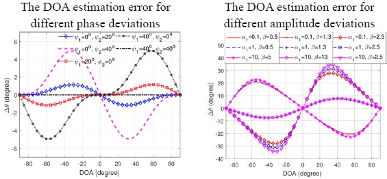
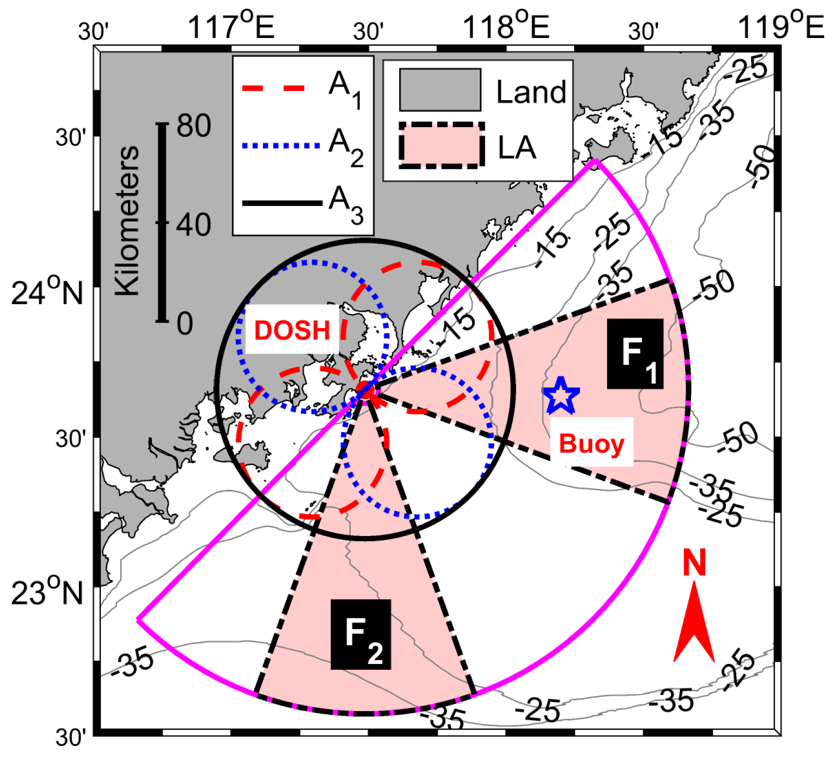
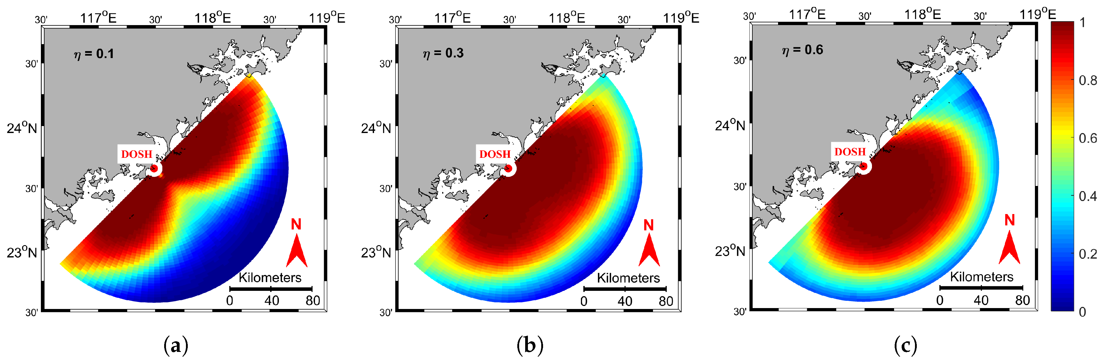
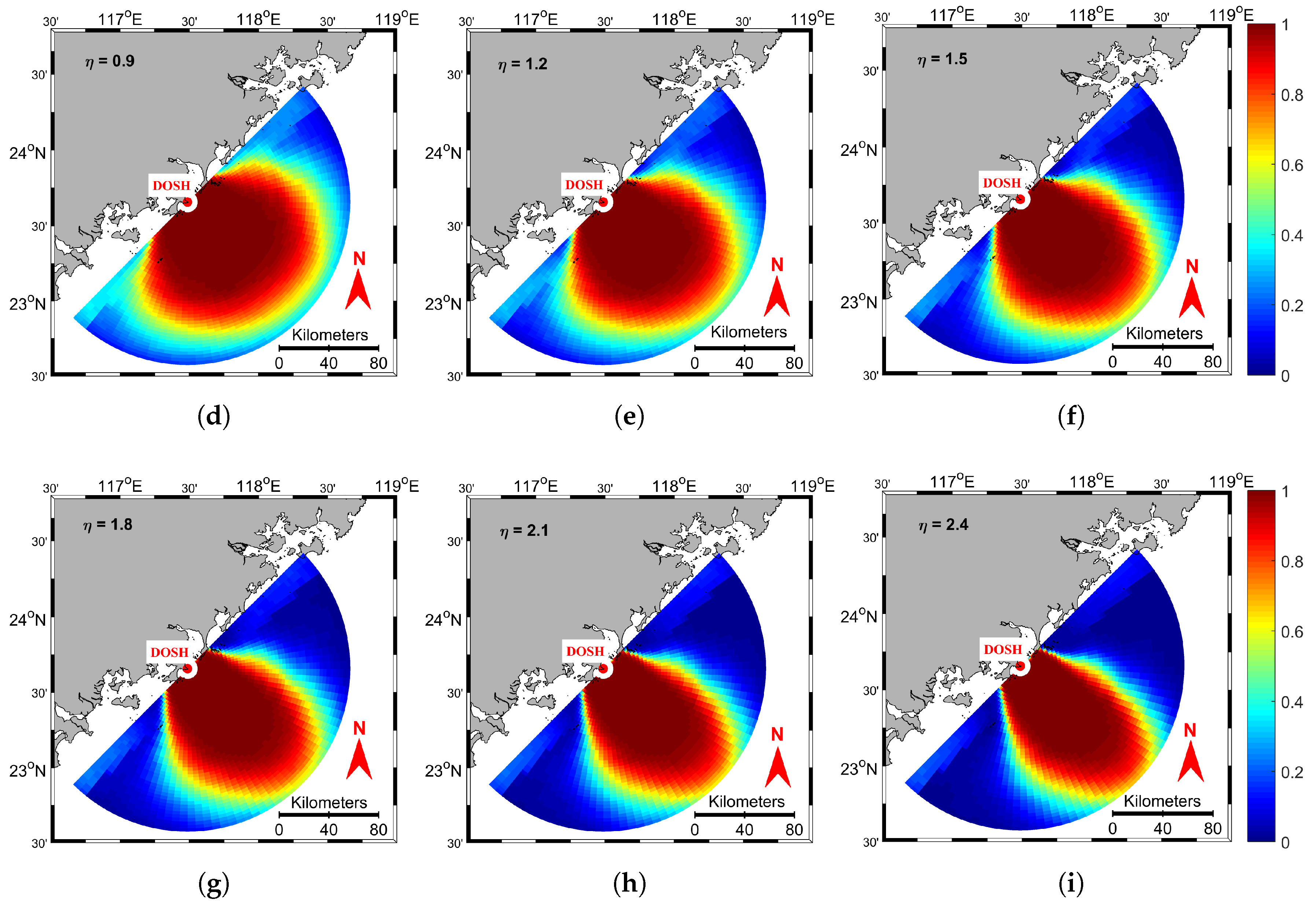
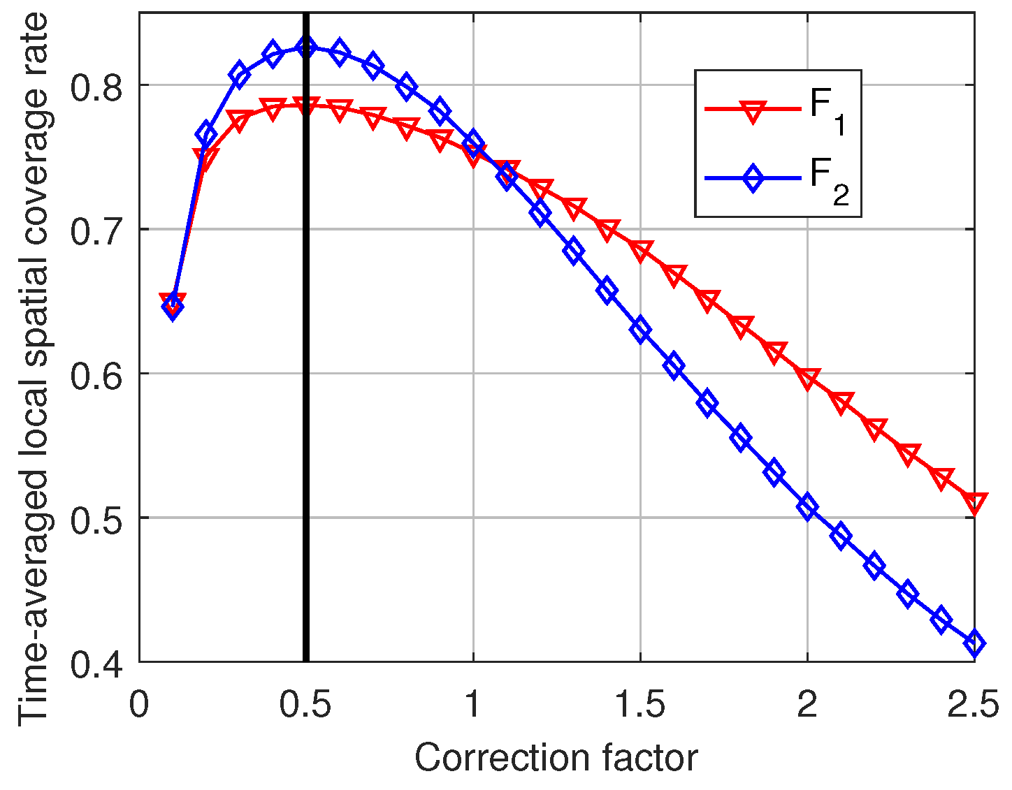
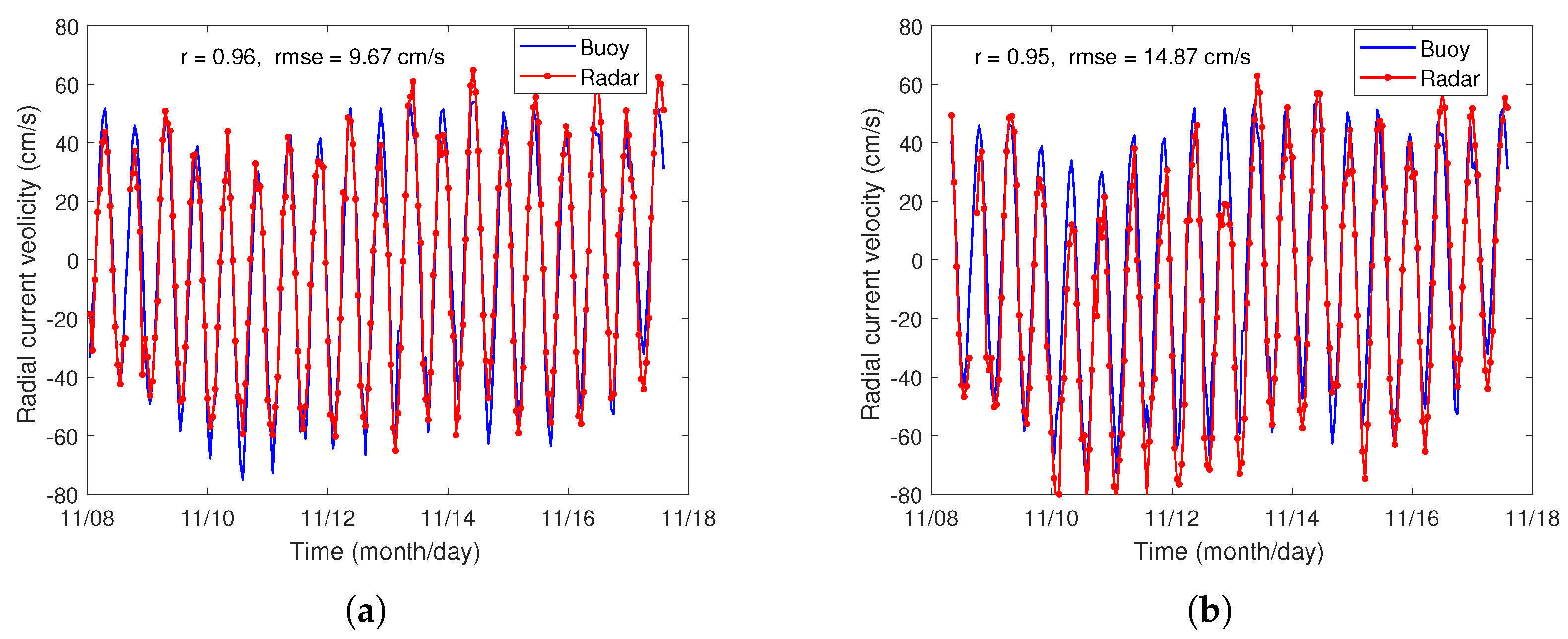
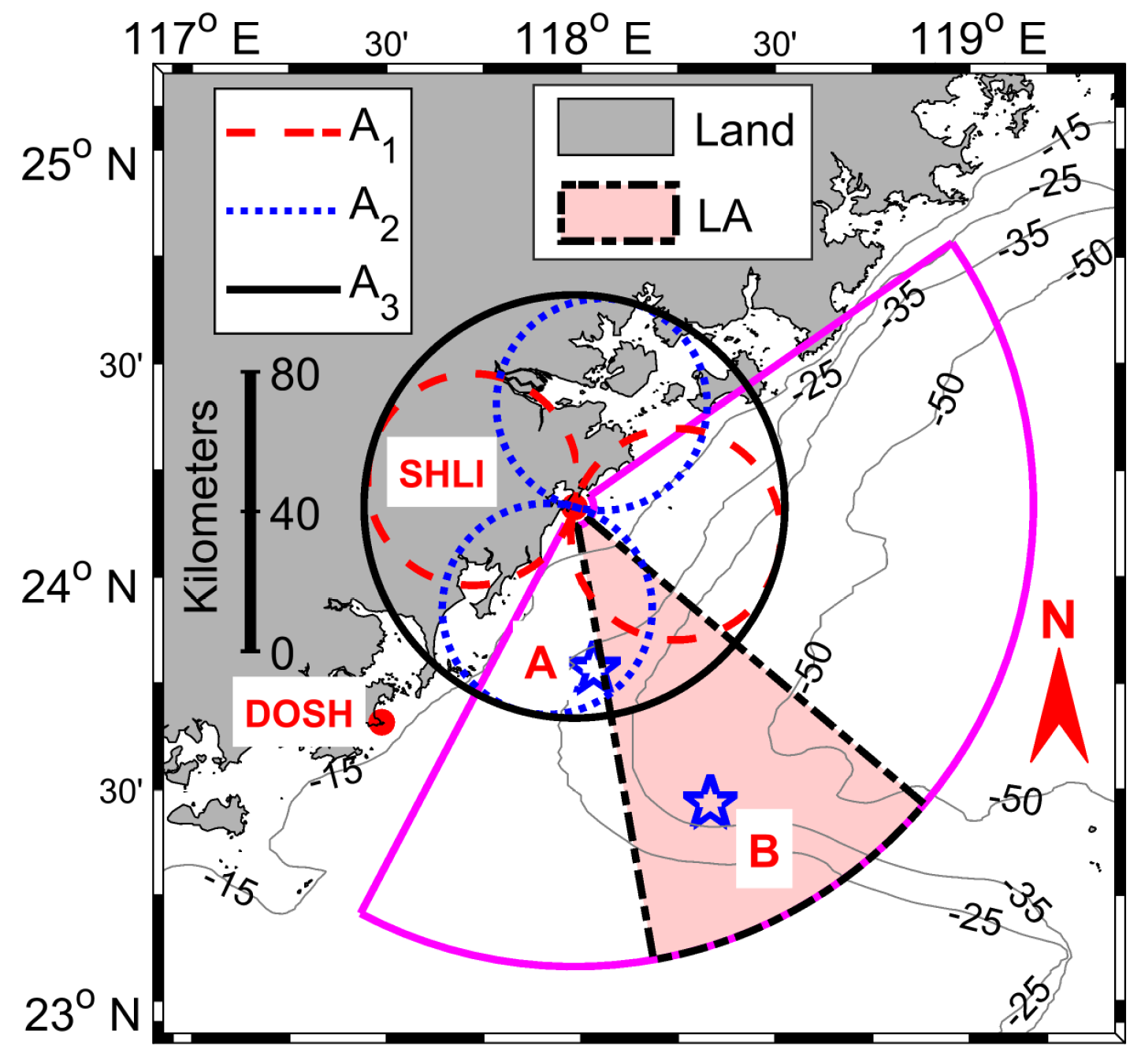
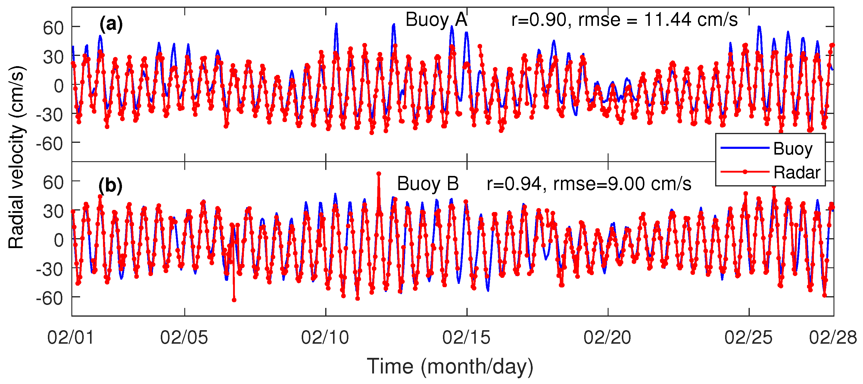
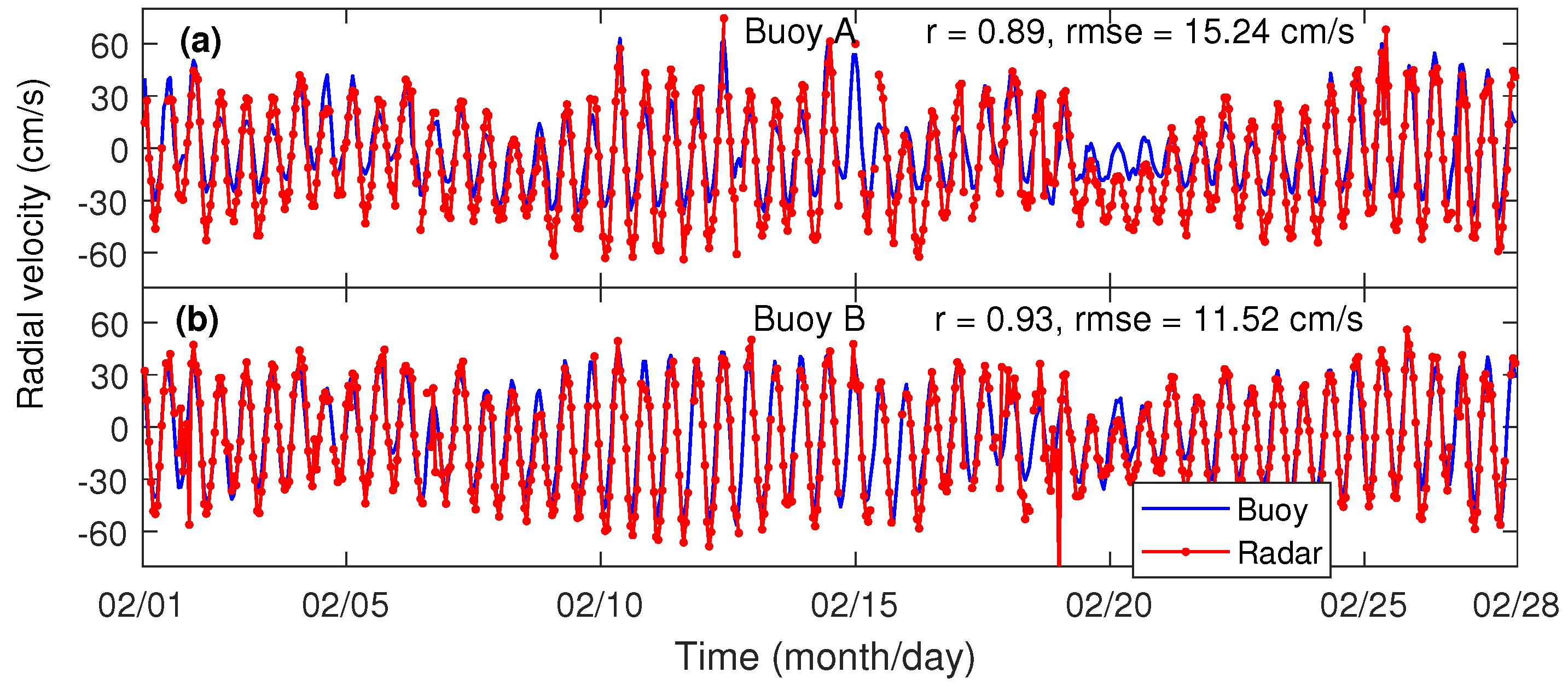
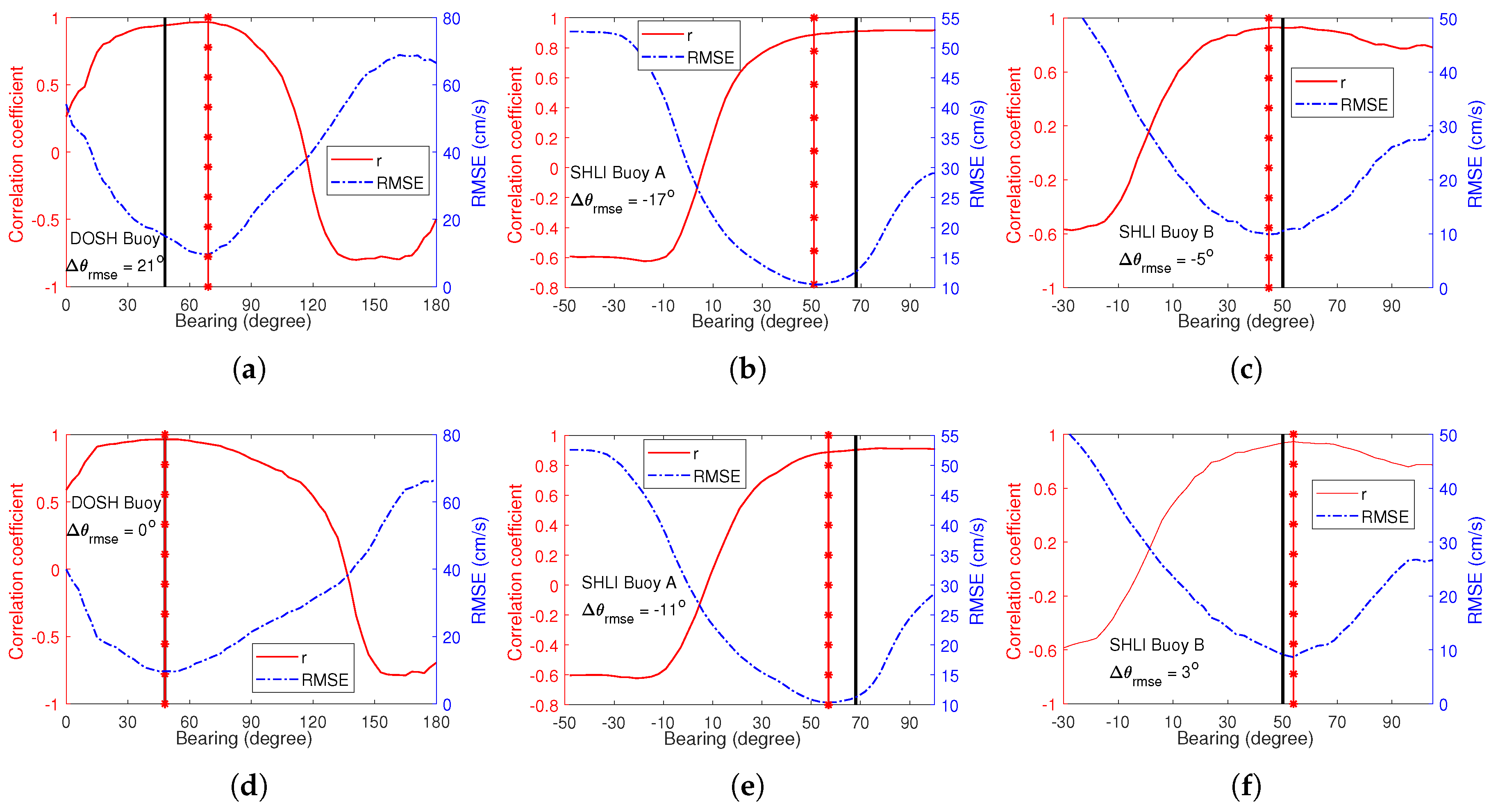
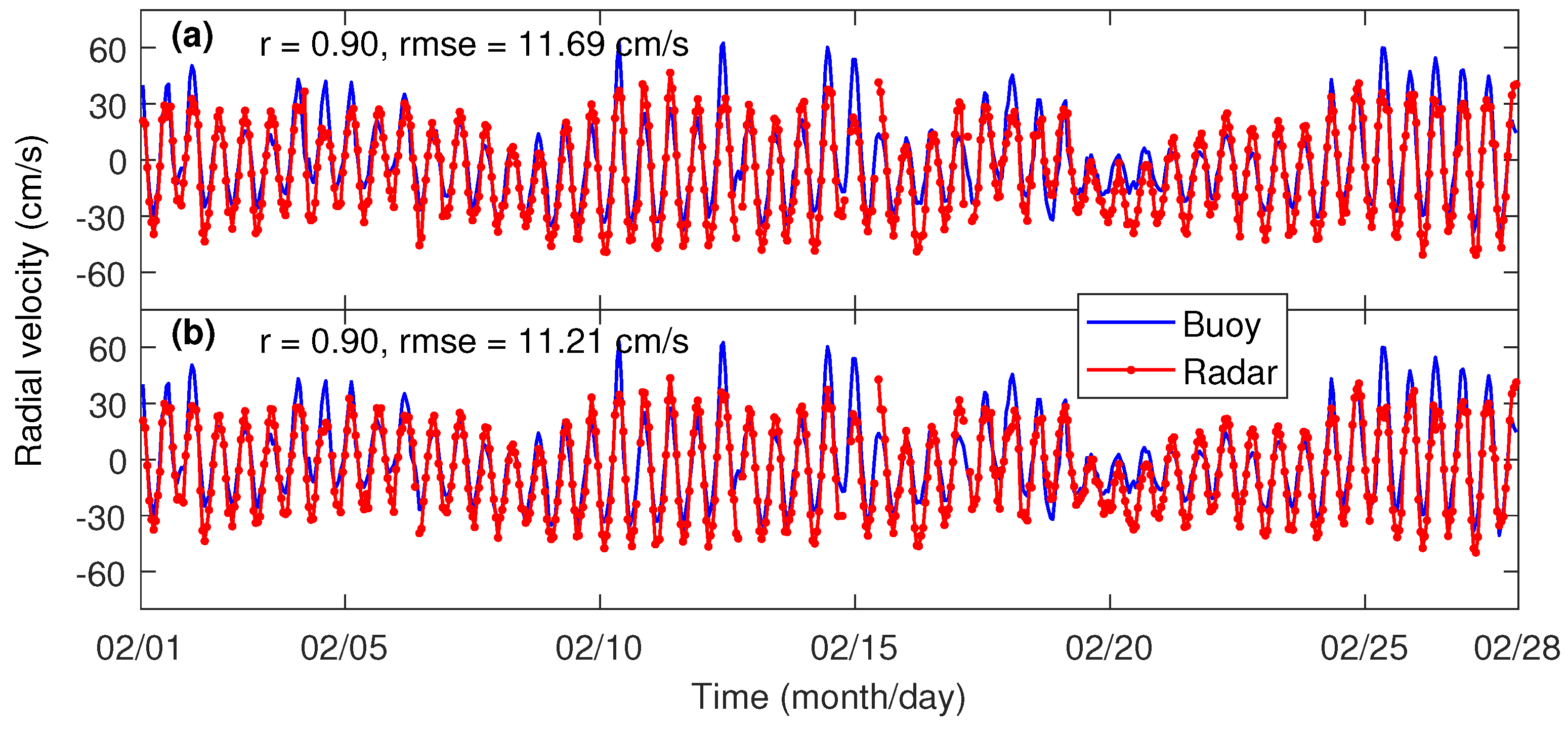
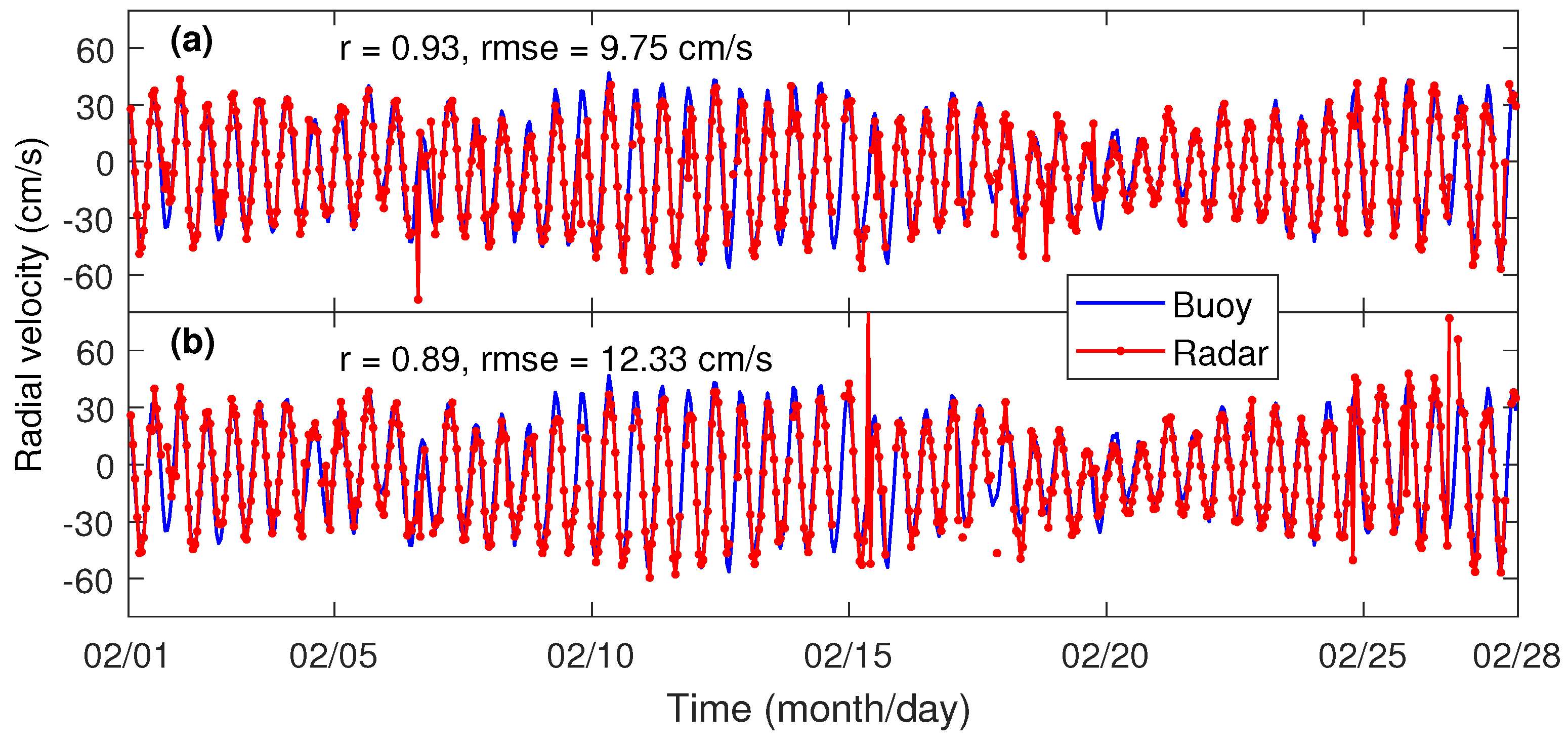
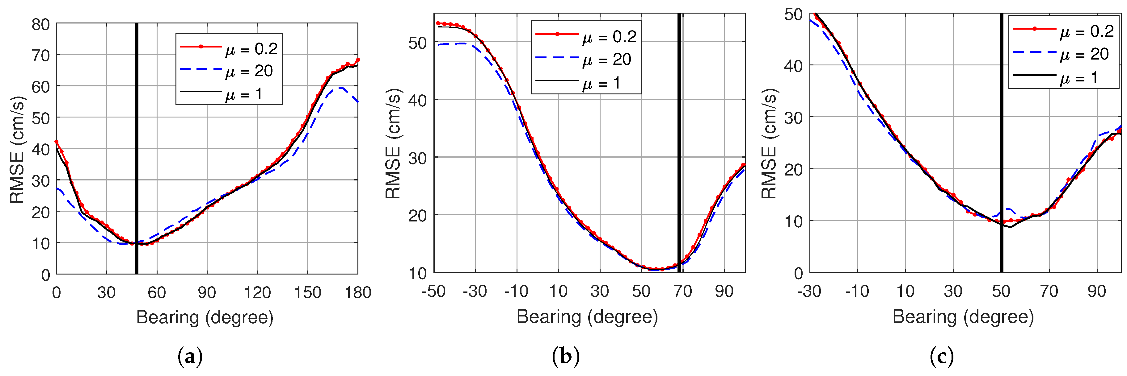
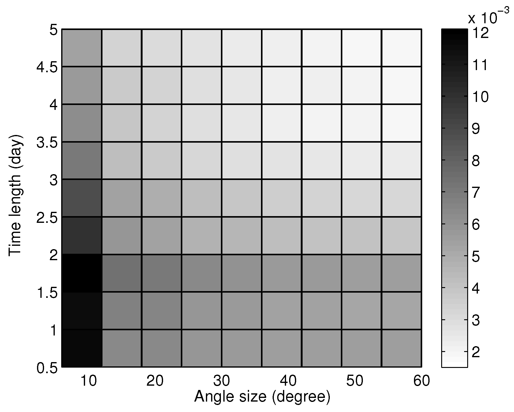
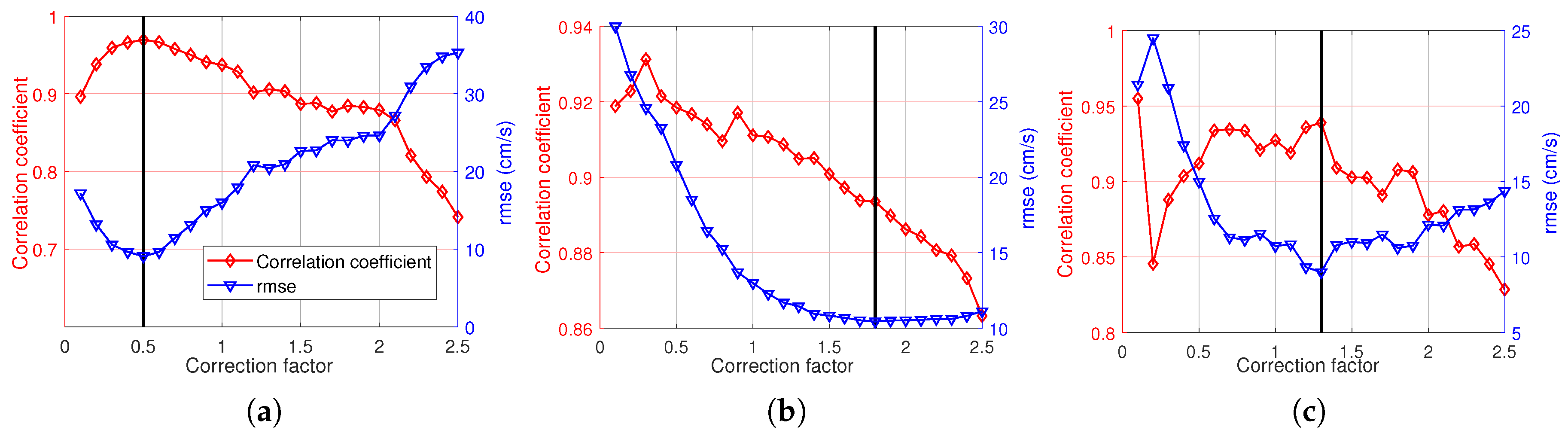
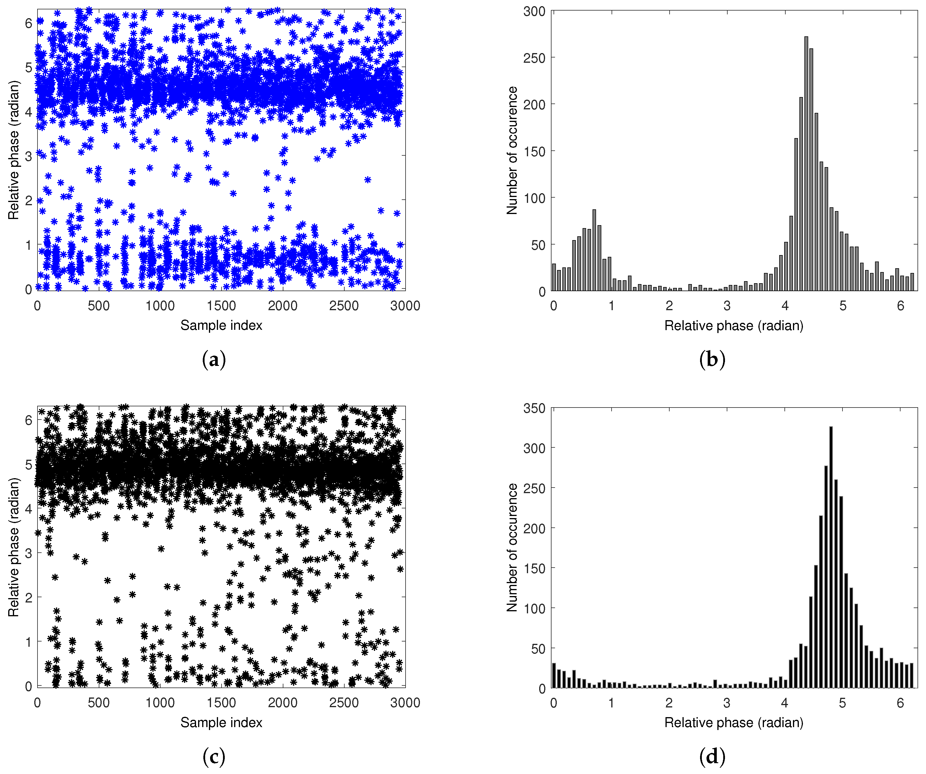
Table 1.
The bearing offset and the ratio of the amplitude deviation of sine loop to that of cosine loop. is the bearing of the buoy to the radar origin. is the bearing offset for the uncalibrated case (Figure 11a–c). is the bearing offset for the calibrated case (Figure 11d–f). is the ratio of the two loops for the calibrated case. is the ratio of the two loops for the uncalibrated case. is the direction-of-arrival (DOA) estimation error calculated by Equation (14) with , , and .
| Site–Buoy | ||||||
|---|---|---|---|---|---|---|
| DOSH–buoy | 48° | 21° | 0° | 1 | 2 | 20.71° |
| SHLI–buoy A | 68° | −17° | −11° | 0.63 | 0.48 | −18.95° |
| SHLI–buoy B | 50° | −5° | 3° | 1.12 | 0.86 | −4.31° |
© 2017 by the authors. Licensee MDPI, Basel, Switzerland. This article is an open access article distributed under the terms and conditions of the Creative Commons Attribution (CC BY) license (http://creativecommons.org/licenses/by/4.0/).
Share and Cite
MDPI and ACS Style
Lai, Y.; Zhou, H.; Zeng, Y.; Wen, B. Quantifying and Reducing the DOA Estimation Error Resulting from Antenna Pattern Deviation for Direction-Finding HF Radar. Remote Sens. 2017, 9, 1285. https://doi.org/10.3390/rs9121285
AMA Style
Lai Y, Zhou H, Zeng Y, Wen B. Quantifying and Reducing the DOA Estimation Error Resulting from Antenna Pattern Deviation for Direction-Finding HF Radar. Remote Sensing. 2017; 9(12):1285. https://doi.org/10.3390/rs9121285
Chicago/Turabian StyleLai, Yeping, Hao Zhou, Yuming Zeng, and Biyang Wen. 2017. "Quantifying and Reducing the DOA Estimation Error Resulting from Antenna Pattern Deviation for Direction-Finding HF Radar" Remote Sensing 9, no. 12: 1285. https://doi.org/10.3390/rs9121285
Note that from the first issue of 2016, this journal uses article numbers instead of page numbers. See further details here.