Abstract
The key to simulating soil erosion is to calculate the vegetation cover (C) factor. Methods that apply remote sensing to calculate the C factor at a regional scale cannot directly use the C factor formula. That is because the C factor formula is obtained by experiments, and needs the coverage ratio data of croplands, woodlands, and grasslands at a standard plot scale. In this paper, we present a C factor conversion method from a standard plot to a km-sized grid based on large sample theory and multi-scale remote sensing. The results show that: (1) Compared with the existing C factor formula, our method is based on the coverage ratio of croplands, woodlands, and grasslands on a km-sized grid, and takes the C factor formula obtained from the standard plot experiment and applies it to a regional scale. This method improves the applicability of the C factor formula, and can satisfy the need to simulate soil erosion in large areas; (2) The vegetation coverage obtained by remote sensing interpretation is significantly consistent (paired samples t-test, t = −0.03, df = 0.12, 2-tail significance p < 0.05) and significantly correlated with the measured vegetation coverage; (3) The C factor of the study area is smaller in the middle, southern, and northern regions, and larger in the eastern and western regions. The main reason for that is the distribution of woodlands, the Hunshandake and Horqin sandy lands, and the valleys affected by human activities; (4) The method presented in this paper is more meticulous than the C factor method based on the vegetation index, improves the applicability of the C factor formula, and can be used to simulate soil erosion on a large scale and provide strong support for regional soil and water conservation planning.
1. Introduction
Soil erosion models have provided strong support for regional soil and water conservation planning. With the development of the Geographic Information System (GIS) and Remote sensing (RS), the water erosion equation has been widely used in regional soil erosion simulations [1,2,3,4,5,6]. Current water erosion models include the universal soil loss equation (USLE) [7], the revised universal soil loss equation (RUSLE) [8,9], the China soil loss equation [10], and so on. These models are being widely used to estimate soil loss in agricultural and environmental management. In the models, soil loss A = R × K × L × S × C × P, where R, K, L, S, C, and P, respectively, are rainfall erosivity (R), soil erodibility (K), slope length (L), slope steepness (S), vegetation cover and management (C), and support practice factor (P). The R, K, L, and S factors are controlled by the natural environment, and therefore will not be changed by short-term soil and water conservation measures and activities. However, the C factor has the greatest change range among the factors of water erosion models, and the changes can differ by two to three orders of magnitude [11]. According to Benkobi et al. [12] and Biesemans et al. [13], the vegetation cover factor, together with slope steepness and length factors, are most sensitive for soil loss, and have the most significant effect on the overall effectiveness of the USLE/RUSLE models [14]. Therefore, calculating and improving the accuracy of regional C factors has become the key to improving regional soil erosion simulations.
Most of the regional C factors have been determined with remote sensing data through the following methods: (1) The direct assignment of land use/coverage [6]. This method is simple, but the accuracy of the computed C factor is poor [11]; (2) The vegetation index estimated C factor method [15,16,17]. This method can express the regional vegetation coverage more finely, but it is less comprehensive, and multiple layers and shallow roots are usually ignored; (3) The spectral mixing analysis (SMA) estimated C factor method [18,19]. The SMA method considers the contributions of litter, gravel, etc.; it can fully reflect the C factor information independent of the measurements, and the soil background does not affect it. However, the SMA method cannot be used when vegetation and/or litter completely covers the surface, or when the data is affected by multiple scattering [11]; (4) Experimental approaches combined with geostatistical methods [17,20]. With this method, the C factor can be interpolated using GIS and remote sensing images as auxiliary variables. Wang et al. [17] improved mapping the C factor for the USLE by geostatistical methods with TM images. Based on multiple primary variables (canopy cover, ground cover, and vegetation height), Gertner et al. [20] mapped the C factor in regions from a joint co-simulation.
All of these methods that apply remote sensing have the following problems: Firstly, the methods above use the C factor formula obtained from standard plot experiments, while such formula cannot be directly applied to an entire region. The C factor formula of croplands, woodlands, and grasslands is calculated by experiments on the erosion rate of cropland, woodland, and grassland plots with bare land in the standard plots. However, the vegetation cover of a region is a complex combination of croplands, woodlands, and grasslands, differing from the vegetation cover modelled in the standard plot. Secondly, the RSI method requires a large number of field samples, and cannot be used in fragmented landscape areas, such as the farming-pasture ecotones of northern China. Not only is it difficult to ensure the accuracy of the spatial interpolation, but it is also time-consuming, laborious, and difficult to promote. Thirdly, there are very few ways to properly consider the effects of surface coverage and canopy coverage on soil erosion in the modelled region.
Based on the results of previous regional C factor estimations, we analyzed the key factors of soil erosion and highlighted the key factors affecting the scale conversion [21]. In order to improve the accuracy of the regional C factor estimation and obtain a large-scale C factor map for a macro-scale soil erosion simulation, we built a C factor estimation method based on large sample theory and Landsat Thematic Mapper (TM) images, and we show that our method solves the key problem of transitioning from a standard plot to km-sized grids, and hence accurately estimates regional C factor.
2. Study Area
The eastern section of the farming-pasture ecotone (hereinafter referred to as the study area) (see Figure 1) includes 84 counties (banners) in the Inner Mongolia Autonomous Region, Liaoning Province, Heilongjiang Province, Jilin Province, and Hebei Province, and has an area of 4.402 × 10⁵ km2. In 2015–2016, our research group carried out two field trips to determine the land use and soil erosion in the study area, and the length of the survey route was nearly 7000 km. According to the typical geographic unit and landform type, we set up 21 survey sample areas. From 19 July to 25 July 2015, the western part of the study area was inspected, where 10 inspection points were created over a route of 2930 km. From 7 August to 14 August 2016, the eastern part of the study area was inspected, where 11 inspection points were created over a route of more than 4000 km.
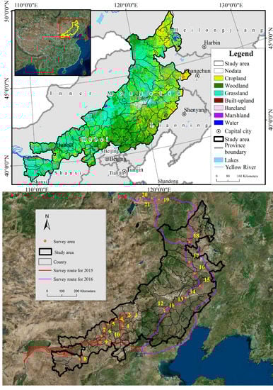
Figure 1.
Study area and two field trips routes.
3. Materials and Methods
3.1. Basic Idea and Research Framework
More than 1000 coverage data-points were obtained from Landsat TM images of the Global Land Survey in 2010 (GLS2010) and ground measurements, and according to large sample theory and information entropy theory, their distributions and proportions are similar. Large sample theory, also called asymptotic theory, is used to approximate the distribution of an estimator when the sample size n is large. This theory is extremely useful if the exact sampling distribution of the estimator is complicated or unknown [22]. In addition, based on information-entropy theory [23], when the sample size is sufficiently large, the samples can be assumed approximate to a normal distribution. According to the above two theories, the subsets of remote sensing data-points and field measurements data-points have a similar distribution. That is, the same km-sized grid, 2000 land cover data-points obtained from field measurements have a similar distribution and similar proportion of croplands, woodlands, and grasslands as 1000 land cover data-points determined from the Landsat TM images. The accuracy of the field measured vegetation cover method is better than that of the remote sensing method, so the field measurements can be used as the reference for verifying the remote sensing measurements. The research framework is shown in Figure 2.
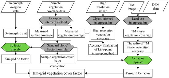
Figure 2.
The C factor conversion method from a “standard plot (single vegetation type)” to a “km-sized grid” (multiple vegetation types).
The C factor conversion from a “standard plot (single vegetation type)” to a “kilometer grid” (multiple vegetation types) contains six steps: (1) The vegetation cover of the sampling method was evaluated based on the high-resolution images of the survey sample area; (2) We interpreted the Landsat TM images of the study area and derived the land use data based on the CART decision tree classification method; (3) We then set up 21 survey sample areas, each with an area of 1 km2, and 2000 canopy cover and surface cover data points were established; (4) Based on the resolution of land use data, 1125 canopy coverage data points were obtained in each km-sized grid of the study area, and the canopy coverage (Cc) of the croplands, woodlands, and grasslands was calculated; (5) The surface cover (Sc) factor was calculated based on the surface coverage surveyed in the survey sample area, and was applied to the entire study area according to the landform type; (6) According to the Cc and Sc factors, we calculated the C factors of the study area. Finally, we verified the regional C factor by the survey sample areas.
3.2. Materials
The study mainly used three types of data: measured data (survey sample data), remote sensing data (Landsat TM image data, MODIS data and high-resolution images), and basic geographical data. We used the Landsat TM image data of the Global Land Survey in 2010 (GLS2010, https://glovis.usgs.gov/, 30 m × 30 m). The dates of the MODIS data (https://urs.earthdata.nasa.gov/profile, 1 km × 1 km) are 12 July 2015 and 27 July 2016, near the survey dates. A total of about 42,000 coverage data-points were surveyed throughout the study area. Basic information on the survey sample areas is shown in Table 1.

Table 1.
The basic information of the survey sample area.
We used Gaofen-2 satellite images (GF-2) that covered the investigation area to discuss the relationship between the survey estimated vegetation coverage and intercept vegetation coverage in the km-sized grid. The GF-2 satellite was designed and developed by the China Academy of Space Technology (CAST). It employs the CAST-CS-L3000A bus and two Panchromatic image/Multi spectral image (PAN/MS) cameras: one produces MS images with four bands in the visible and near-infrared (VNIR) range with a spatial resolution of 3.2 m; and the other generates PAN images in the visible range with a spatial resolution of 0.8 m [24]. We chose four GF-2 images that were obtained within one month either side of the survey date in 2015. The GF-2 date of sample NO. 4 is 4 August 2015, sample NO. 5 is 9 August 2015, sample NO. 9 is 19 August 2015, and sample NO. 10 is 9 August 2015. With the eCognition software, we adopted the object-oriented high-precision remote sensing interpretation method to obtain high-resolution land use/cover data of the survey sample area.
3.3. Methods
3.3.1. Canopy Coverage Factor Upscaling
The canopy coverage factor can be calculated from vegetation cover, which can be estimated using point intercept, line-point intercept, grid-point intercept, and ocular estimates [25,26]. Scholars have compared the above-mentioned methods to calculate the vegetation cover, and found that when the samples are less than 20, the point-based methods are more precise than ocular estimates [25,27,28] and line-point intercepts [25]. When the sample size is large enough, the estimate of the line-point intercept is the same as that of the point intercept and grid-point intercept, and can correctly reflect vegetation cover [25,26]. In this paper, 21 survey sample areas were set up in the study area. In each survey sample area we collected a total of 2000 samples, which is far greater than the requirement of 20 samples [26].
The size of the sampling unit is also important for ground measurements. Duncan et al. [29] analyzed the influence of sampling unit size on the remote sensing regression model based on the vegetation index and vegetation cover, and discussed the most suitable sampling unit size. In this paper, we chose the km-sized grid as the statistical unit. Then, via TM image interpretation, we produced more than 1000 land use/land cover data-points in each km-sized grid. Next, the MODIS vegetation cover was directly measured from the vegetation index in the km-sized grid. The different methods used to estimate vegetation cover are shown in Figure 3.
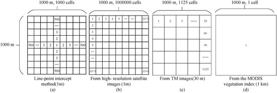
Figure 3.
The different methods used to estimate vegetation cover in the survey sample area: (a) The line-point intercept method; (b) from high-resolution satellite images; (c) from TM images; (d) from the MODIS vegetation index.
The key to estimating the C factor is to calculate the vegetation cover. There is no standard method to monitor vegetation cover, and current methods can be divided into surface measurement methods and remote sensing methods. The surface measurement method is limited by the workload and the measurement area size, and is unsuitable as an independent measurement method at a large scale. The methods based on remote sensing to calculate the vegetation cover rely on a surface test for the regression calibration. It has a certain accuracy, but is subject to the restrictions of promotion and application, especially in fragmented landscapes like farming-pasture ecotones. In terms of current technology, the accuracy of the surface measurement method is higher than that of the remote sensing method, and thus can be used as the basis for remote sensing measurements and data verification [30].
3.3.2. TM Image Land Use Interpretation
• Land use classification system
The coverage and proportion of various land types on a km-sized grid can be calculated according to the high-resolution land use data of the study area, such as the global 30 m land use data produced by Chen et al. [31] or Gong et al. [32]. However, both the above-mentioned classification data confuse grassland and bare land in the study area, and contain no secondary classification of grassland. Therefore, we adopted a secondary land use classification system for the study area based on the land use/cover classification system of Liu et al. [33] to classify the TM images. The interpretation effects of some classification methods (such as neural network classification, object-oriented classification) can be very good for a single image, but when it comes to a large area, the workload and classification efficiency must be considered. The CART algorithm is based on the decision tree classification method [34], and combines DEM and NDVI data, as well as supervised and unsupervised classification methods, resulting in a much higher interpretation efficiency than other interpretation methods [34] for large areas. So, we adopted the decision tree classification method of the CART algorithm to carry out land use classification (we interpreted more than 40 scene Landsat TM images from GLS2010).
• Decision tree classification based on the CART algorithm
Prior to classification, the Landsat TM and Landsat Enhanced Thematic Mapper (ETM) data in the Global Land Survey of 2010 (GLS2010) underwent cloud interpretation and geometric correction were combined into multi-band images composed of blue, green, red, near infrared, short-wave infrared, medium-wave infrared, and long-wave radiation, together with NDVI, ISODATA, DEM, and other bands. The NDVI data was generated from TM images and the DEM data from global ASTGTM data. The ISODATA data is from unsupervised classification of the TM images, and the minimum class number of unsupervised classification is 10 and the maximum is 25.
The main steps of decision tree classification based on the CART algorithm are: (1) Select the training areas. According to the secondary classification system, a certain number of training samples were selected in the multi-band image and used to obtain expert knowledge rules. The training area selection order was: (i) water (river canals); (ii) built-up lands, industrial and mining lands, residential lands (urban land, rural residential areas, other construction land); and (iii) croplands (irrigated land, dry land); (2) Establish a decision tree based on the training area. We used the extension tool RuleGen [34] to automatically generate decision tree rules, and used the ENVI Execute Existing Decision Tree tool to establish a decision tree for land use interpretation.
• Classification accuracy evaluation
In this paper, the study area is relatively large and it is difficult to carry out scientific random field verification, so this paper uses a large number of random distributions of the single pixel verification point method based on Google images [31,35]. We generated a total of 2000 points randomly throughout the study area (50 points in each image). In order to obtain the real surface cover data of the random points, and considering the high accuracy of Google images, we first used Google Earth to distinguish the real surface cover data [31,35], and second, we moved the random verification point which is in the edge of land cover type, to the center of land cover type, and avoided mixing pixels, ensuring the accuracy of the true surface data. Finally, we used the true surface data of points randomly to verify the accuracy of the land use in the interpretation.
3.3.3. Surface Coverage Factor Upscaling
At regional scale, it is difficult to obtain surface cover information such as surface litter, crop stubble, and gravel required by soil erosion models. To overcome this limitation, we first set up 21 survey sample areas in the typical landform unit, measured the ratio of surface litter, crop stubble, and gravel in the sample area, and finally interpolated them according to land surface types to obtain the surface coverage factor in the study area. Secondly, the surface of the study area was classified according to the geomorphic map (1:4 million) of China and its adjacent areas. Thirdly, according to the natural geographic features of the study area, we found that the surface of the study area can be classified by the geomorphic unit that can reveal the surface cover information to calculate the vegetation cover. Lastly, the surface coverage (Sc) of the study area was calculated based on the field coverage of the survey sample area and the structure geomorphic unit of the study area, as shown in Figure 4.
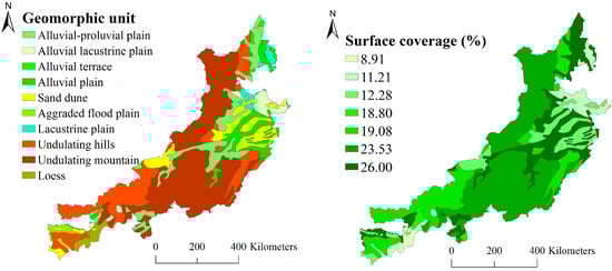
Figure 4.
The coverage of surface matter in the study area.
3.3.4. Regional Vegetation Cover Factor
• Standard plot C factor algorithm
Many scholars have experimentally determined the standard plot C factor for different regions [4,7,11,36]. Different formulas are given based on different vegetation covers, for example: Jin et al. [37] built the C factor formula of grassland that had a 1.9% coverage in the standard plot of the Huangfu River Basin; Jiang et al. [38] built the C factor formula of grasslands and woodlands in a standard plot with coverages of more than 5% in Ansai County of Shaanxi Province; Liu [39] built the C factor formula of croplands, woodlands, and grasslands in a standard plot in Beijing.
The surface cover is mainly composed of litter, crop stubble, and gravel, which are more effective in reducing soil erosion than plant canopy cover. Based on this, the C-factor algorithm of Liu [39] considers both the surface cover and canopy cover of croplands, woodlands, and grasslands, which makes the C factor result more objective. Therefore, we chose Liu’s [39] standard plot vegetation cover factor algorithm to calculate the C factor, as shown in Equation (1).
The canopy cover factor of cropland and grassland is calculated by Equation (2), and the canopy cover factor of woodland is calculated by Equation (3). Liu [39] found that the Sc factors of croplands and grasslands can be combined into a single formula by Equation (4). The Sc factor of woodlands is calculated by Equation (5).
where Cc and Cs are the canopy cover factor and the surface cover factor, respectively; Vc and VR are the canopy cover (%) and surface cover (%), respectively; and h is the canopy height (cm). As it is difficult to obtain surface information such as litter, crop stubble, and gravel on the regional scale, in this paper, the Sc factor was calculated by using the surface coverage factor upscale method.
• Regional C factor algorithm
The regional vegetation cover factor needs to be calculated based on the fractional cropland, woodland, and grassland coverage. Based on the C factor algorithm of the standard plot, the regional C factor algorithm is proposed, as shown in Equation (6).
where C is the C factor of the km-sized grid, Vcrop is the cropland coverage (%), Vgrass is the grassland coverage (%), and Vforest is the forest coverage (%). Ccrop is the cropland vegetation cover factor, Cgrass is the grassland vegetation cover factor, and Cforest is the woodland vegetation cover factor.
4. Results
4.1. C Factor of the Survey Sample Area
Based on land use data and surface cover data, the C factor of each survey sample area was calculated according to the C factor algorithm (Table 2).
Table 2.
The C factor of the survey sample area.
It can be seen that the C factor of the sample area that has a higher proportion of woodland was smallest. The C factor of the survey sample areas that have a higher proportion of grassland and cropland cover was medium, and the C factor of the survey sample areas that have a higher proportion of unused land (sand and bare land) was highest.
4.2. Fractional Vegetation Cover (FVC) in the Study Area
Based on the 30 m resolution land use map in 2010 from GLS2010, we calculated the coverage proportion of cropland, woodland, and grassland, as well as the vegetation cover of the study area, as shown in Figure 5. According to the vegetation cover of the study area in 2010 based on GLS2010, the vegetation cover (including the ratio of cropland, woodland, and grassland) was extracted in each survey sample area and verified by the measured vegetation coverage, as shown in Figure 6. The correlation vegetation coverage between the remote sensing and measured points is shown in Table 3. The paired-samples Student’s t-test was used to detect the statistical significance level of the remote sensing interpretation vegetation cover. The results are shown in Table 4.
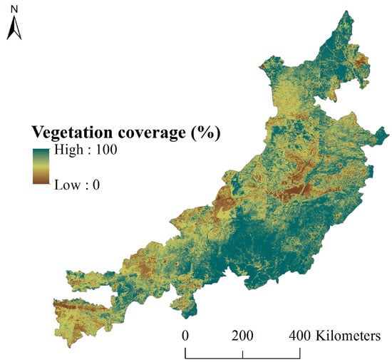
Figure 5.
Vegetation coverage in the study area (2010).
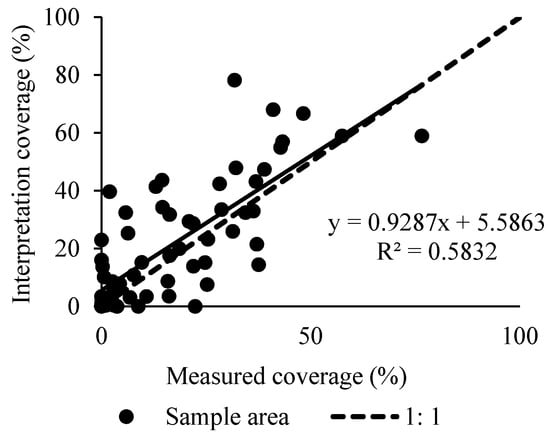
Figure 6.
The verification of vegetation coverage in the survey sample area.
Table 3.
The correlation between the remote sensing interpretation and measured vegetation coverage.
Table 4.
The paired-samples Student t-test.
It can be seen from Figure 6, as well as Table 3 and Table 4, that the vegetation coverage obtained by the remote sensing interpretation is significantly consistent and significantly correlated with the measured vegetation coverage. The vegetation coverage obtained by remote sensing interpretation is significantly consistent with the measured vegetation coverage (paired samples t-test, t = −0.03, df = 0.12, 2-tail significance p < 0.05), where R2 is 0.58. Simultaneously, there is a statistically significant linear relationship present between the two groups of data. The two groups of data are significantly correlated (significance p < 0.05), and the correlation is 0.76. Furthermore, the two groups of data are generally distributed near the 1:1 line, and the regression coefficient is 0.93. To sum up, the results show that the method in this study can help accurately obtain the coverage ratio of croplands, woodlands, and grasslands in the km-sized grid.
4.3. C Factor in the Study Area
Based on the C factor conversion method, and using the proportional coverage of croplands, woodlands, and grasslands in the km-sized grid, the C factor in the study area (2010) was calculated, as shown in Figure 7.
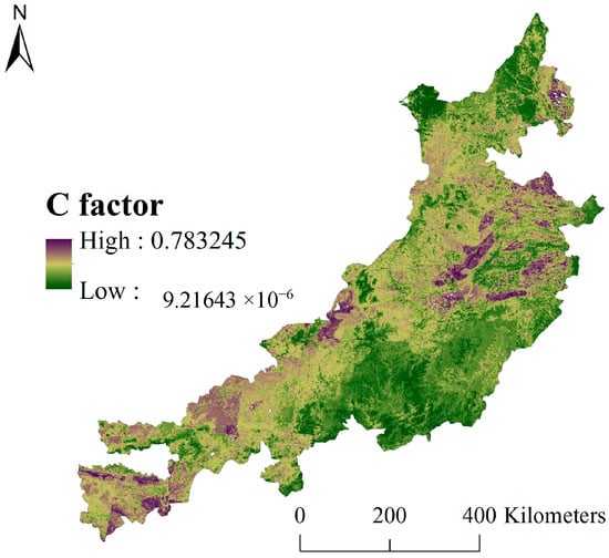
Figure 7.
The C factor in the study area (2010).
It can be seen from Figure 7 that the C factor is smaller in the middle, southern, and northern regions, and larger in the eastern and western sections of the study area. In the central and northern parts of the study area, there are a large number of woodlands, making the C factor lower. The Hunshandake sandy lands and Horqin sandy lands result in larger C factors in the eastern and western regions. In the south-central part of study area, the C factor of woodlands is obviously smaller than that of valleys. The main reason is that valleys are affected by human cultivation, so the C factor is improved. Using the C factor based on the measured coverage, the C factor of the survey sample area based on remote sensing interpretation is verified (Figure 8).
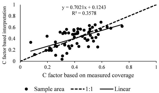
Figure 8.
Verifying the C factor based on remote sensing interpretation.
It can be observed in Figure 8 that the C factor of the survey sample area calculated via remote sensing is consistent with the one based on measured coverage. The two data are distributed near the 1:1 line, with R2 = 0.36 and correlation coefficient = 0.7. Due to the resolution and interval differences among the TM images and the field measurement, we obtained a low R square, which is acceptable if we do not use it to predict the C factor. This shows that the C factor measured in this study can reflect the vegetation cover in the study area and can be used to calculate the C factor in the soil erosion equation.
5. Discussion
5.1. Relationship between Line-Point Estimated Vegetation Coverage and Intercept Vegetation Coverage in the Km-Sized Grid
With the eCognition software package, we used the object-oriented classification method to interpret the high-precision images (Gaofen-2 satellite images (GF-2)) of the sample area and obtain the coverage of various land cover types. The cropland, grassland, and woodland coverage obtained from high-precision images was compared with the line-point intercept estimated data, as shown in Figure 9.
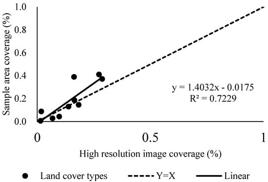
Figure 9.
The correlation between the measured Fractional Vegetation Cover (FVC) from the line-point intercept method and the high-resolution image interpretation.
It can be seen from Figure 9 that the correlation between the FVC from the line-point intercept method and the high-resolution image interpretation is very high. The two groups of data are mainly distributed in the vicinity of the 1:1 line. The nonparametric test of the relevant sample Wilcoxon, shows that the two groups of data are significantly consistent at a significance level of p < 0.05. The value of R2 is 0.72 and the slope is 1.40, indicating that the cropland, grassland, and woodland coverage obtained from the line-point intercept method is larger than that from image interpretation, but can still be used to reflect the proportion of cropland, grassland, and woodland in the study area, with an interpretation rate of 72.29%. This result is basically consistent with the findings of previous studies [25,26], indicating that the line-point intercept method can effectively reflect the coverage of cropland, grassland, and woodland in the survey sample area.
5.2. Comparison of Our Method and the C Factor Algorithm Based on Remote Sensing Vegetation Index
We compared the C factor derived from the vegetation index (see Appendix A), with the C factor determined by our method, and the difference of two C factors is shown in Figure 10.
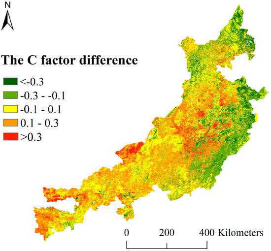
Figure 10.
The difference of C factors based on the vegetation index and remote sensing data.
It can be seen from Figure 7, Figure 8, Figure 9 and Figure 10 that the C factors obtained from the two methods are basically consistent (considering the system errors of vegetation index and remote sensing data, we define C factors with the difference between −0.1 and 0.1 as the consistent) in 22% of the study area. Compared with the C factor derived from image interpretation, the C factor based on the vegetation index is higher (up to 0.3) for western sandy lands, while lower (up to 0.3) for eastern croplands in our study area. The main reason for the differences is that the C factor formula of the standard plot is different. The C factor algorithm based on the vegetation index assumes only one vegetation type in the km-sized grid, and calculates the coverage of the vegetation to obtain the C factor. Therefore, in the sandy area where the complete distribution of sand is assumed, the C factor is overestimated, while in cropland areas where the complete distribution of cropland is assumed, the C factor is underestimated. As such, the C factor based on the remote sensing data is more precise than that based on the vegetation index.
5.3. Uncertainties of the Calculated C Factors
5.3.1. The Empirical Parameters of the C Factor Need to Be Further Confirmed
The water erosion equation used in this paper is a small-scale method, and although many previous studies have applied it on regional scale, many of its parameters are empirical, and their rationality has not been confirmed: (1) The measured parameters of the C factor are for selected field survey times and areas. The C factor in this paper was obtained from remote sensing and field survey data. The summer months (mainly July and August) in the study area have the strongest water erosion throughout the year, and there was almost no water erosion in other months. Besides, the vegetation coverage is higher in summer. The summer C factor determined the accuracy of the water erosion simulation. Therefore, the field investigation time and TM image acquisition time of this study were from July to August; (2) Empirical parameters of the C factor obtained from remote sensing data. The coverage of cropland, woodland, and grassland was obtained by interpreting the remote sensing images and then calculating the proportion of land use/cover. The grasslands can be divided into high coverage, medium coverage, and low coverage grassland [33]. Among them, the high coverage grassland has a coverage of over 50%, assumed as 80%; the medium coverage grassland has a coverage of 20–50%, assumed as 50%; while the low coverage grassland has a coverage of 5–20% of the grass, assumed as 20%. The croplands are classified as irrigated and dry lands. The woodlands are divided into woodlands and shrubs and the coverages of cropland and woodland vegetation are assumed to be 100%. Swamps are low-lying wetlands, which are different from other unused lands (bare land, quicksand, saline, and alkaline land), while similar to high coverage grassland, with an assumed coverage of 80%. These vegetation coverage parameters are empirical to some degree and should be further confirmed in a further study.
5.3.2. Differences between the Remote Sensing Image Coverage and the Measured Coverage
Based on high-precision field survey and remote sensing image interpretation, this study constructed a km-sized grid C factor algorithm. Although the land cover data obtained from TM image interpretation already had the highest resolution on a regional scale, the coverage was still different from the measured coverage because TM images contained mixed pixels. In addition, based on TM images, we can only measure the canopy coverage, rather than the surface coverage that has impacts on soil erosion [39]. Furthermore, the regional surface coverage can currently only be determined based on the surface coverage of representative sites through upscaling.
5.3.3. The Accuracy of the TM Image Interpretation
In this study, we randomly generated points in the TM images to verify the accuracy of our land use interpretation. A total of 2000 verification points (50 in each image) were generated in the study area, where each verification point was a single pixel. Based on the high-precision Google Earth images, we determined the land use type of each verification point to obtain the verification data. In order to ensure the accuracy of the verification data and to reduce the mixed pixel problem caused by the resolution difference and time inconsistency of the verification data, we moved the random points at the edge of the land use units to the center of the land use type. Using the randomly generated 2000 verification points, we tested the interpreted 2010 land use data. The results are shown in Table 5.
Table 5.
Accuracy of land use interpretation in the study area.
It can be seen from Table 5 that the interpretation accuracy is 72.25% and the Kappa coefficient is 0.62. Landis and Koch [40] point out that a Kappa coefficient larger than 0.6 indicates a good accuracy, thus the interpretation accuracy of this paper is good. Many papers have proved the remote sensing interpretation of a large region of low accuracy [31,35]. For example, the accuracy of many automatic classification methods is generally less than 65% [31], and this paper is a study of the fragmented landscape areas for the ecological transition zone, so a 72.25% accuracy is high enough.
There are several problems in the interpretation of land use in the study area: (1) The problem of mixed pixels and different spatial resolutions among Landsat TM and Google earth images decrease the interpretation accuracy; (2) Problems arising from different types of land have the same type of spectrum. The spectra of unused lands and construction lands are relatively close, and on a large regional scale the proportion of construction lands is relatively low, so erosion is rarely influenced. Unused lands such as bareland will cause erosion. However, this paper studied the vegetation cover (C) factor which is related to vegetation (cropland, grassland, and woodland), so the misclassification of construction land and bareland, though it may have resulted in a low accuracy, did not affect the vegetation coverage calculation. So the error can be ignored since this paper focuses on the proportion of vegetation (i.e., croplands, woodlands, and grasslands); (3) The mosaic problem. Due to the phase differences of TM images, there exist edge snap problems between different TM images. These problems reduced the accuracy of the TM image interpretation, so that the results had some uncertainty in the edge areas. However, the overall interpretation accuracy of cropland, woodland, and grassland can meet the requirement of vegetation coverage and the C factor calculation.
6. Conclusions
The vegetation cover (C) factor is one of the most influential factors in the soil erosion model. The C factor derived from a standard plot cannot be directly used on a regional scale. Based on remote sensing data and field investigations, we designed a C factor conversion method from the standard plot to a km-sized grid based on large sample theory. It can be concluded that: (1) Compared with existing C factor algorithms, our algorithm improves the applicable range of the C factor formula of the standard plot, and can be used to simulate soil erosion in large areas; (2) The vegetation coverage obtained by remote sensing interpretation is significantly consistent (paired samples t-test, t = −0.03, df = 0.12, 2-tail significance p < 0.05) and significantly correlated with the measured vegetation coverage. Meanwhile, the line-point intercept method can be used to effectively obtain the vegetation coverage of cropland, woodland, and grassland in the survey sample area (p < 0.05); (3) The C factor of the study area is smaller in the middle, southern, and northern regions, and larger in the eastern and western sections. The main reason for this is the distribution of woodlands, the Hunshandake and Horqin sandy lands, and human cultivation that affects the valleys; (4) The C factor conversion method based on large sample theory is better than the one based on vegetation indices.
In this paper, a method for estimating the regional C factor was proposed by combining the interpretation of remote sensing data and data obtained from field investigations. Our method is limited by the resolution of the remote sensing data, and the accuracy of the TM image interpretation. Thus, in the future, we aim to develop our method by: (1) further confirming the empirical parameters of the C factor; (2) establishing a database of C factors in different seasons; (3) studying the differences between remote sensing and high precision measured vegetation coverage.
Acknowledgments
This study was supported by the National Natural Science Foundation of China (Project No. 41271286), the National Key Research and Development Program (No. 2016YFA0602402), and the Natural Science Foundation of Zhejiang Province, China (LQ18D010003). Thanks to the people from Beijing Normal University: Bo Chen, Gangfeng Zhang, LiLi Lv, Fengfang Chen, Feng Kong, Yongchang Meng, Zhu Wang, Mengyang Li, Mengjie Li, Zhao Liu, Jiayi Fang, Fan Liu, Xu Yang, ZhuoRong Ying, Hao Guo, Yibo Luan, Bank Hu, Jie Zhang, and others, for taking part in investigating the vegetation Coverage in the Eastern Section of the Farming-pasture Ecotone of Northern China. The valuable comments and suggestions from the editor and anonymous reviewers are also greatly appreciated.
Author Contributions
Degen Lin conceived the entire paper, analyzed the data, and designed the experiments. Yuan Gao, Yaoyao Wu, and Huiming Yang analyzed the data and polished the text. Peijun Shi provided technical support, polished the text, and provided project support. Jing’ai Wang provided technical support.
Conflicts of Interest
The authors declare no conflict of interest.
Appendix A. The C Factor Algorithm Based on the Remote Sensing Vegetation Index
1. Calculate Vegetation Coverage Based on the Vegetation Index
In order to express the vegetation coverage of the study area, the MODIS EVI vegetation index needs to be partitioned according to the measured vegetation coverage to carry out the regression modeling. These regression models are generally applicable to the area where the relational expression is constructed. Therefore, the difference between the EVI vegetation index of MODIS and the measured vegetation coverage (hereinafter referred to as FVCD) was used to divide the vegetation index and the measured coverage model. Based on the natural geographical conditions and factors, we analyzed the relationship between the dryness grade, landform type, vegetation type, and sand land, and used the Pearson correlation of FVCD, as shown in Table A1.
It can be seen from Table A1 that the degree of dryness has the highest correlation, where the Pearson’s correlation coefficient of FVCD is 0.386, which is significant at the p < 0.05 level. Therefore, we have established a regression relationship between the vegetation index and the measured vegetation coverage under different dryness grades. The study area is an arid and semi-arid region. The dryness can be subdivided into dryness 1 (0.2–0.4), dryness 2 (0.4–0.44), and dryness 3 (0.44–0.5). According to the degree of dryness, the relationship between the vegetation index and measured vegetation coverage was established, as shown in Table A2 and Figure A1.

Figure A1.
Relationship between the EVI and measured vegetation coverage under different dryness: (a) Dryness grade 1; (b) Dryness grade 2; (c) Dryness grade 3.
Table A1.
The Pearson Relationship between Different Geographical Elements and FVCD.
Table A1.
The Pearson Relationship between Different Geographical Elements and FVCD.
| Different Geographical Elements | Dryness Degree | Sand Land or Not | Landform Type | Vegetation Type | |
|---|---|---|---|---|---|
| Pearson correlation | 0.386 * | −0.206 | 0.114 | −0.283 | |
| Significance (2-tail) | 0.012 | 0.190 | 0.473 | 0.069 | |
* Significance level of 0.05.
Table A2.
The EVI coefficient and measured vegetation coverage under different dryness grades.
Table A2.
The EVI coefficient and measured vegetation coverage under different dryness grades.
| Dryness Grade | Unstandardized Coefficient | Normalization Coefficient | t | Significance | ||
|---|---|---|---|---|---|---|
| B | Standard Error | Beta | ||||
| Dryness 1 | (constant) | 0.263 | 0.075 | 3.516 | 0.003 | |
| EVI coefficient | 0.938 | 0.201 | 0.780 | 4.667 | 0.000 | |
| Dryness 2 | (constant) | 0.548 | 0.046 | 11.903 | 0.000 | |
| EVI coefficient | 0.347 | 0.122 | 0.633 | 2.836 | 0.015 | |
| Dryness 3 | (constant) | 0.406 | 0.122 | 3.336 | 0.009 | |
| EVI coefficient | 1.009 | 0.356 | 0.687 | 2.839 | 0.019 | |
The dependent variable is the measured vegetation coverage.
Table A2 expresses the regression equation of the EVI and measured vegetation coverage relative to the dryness classification and its significance. When the dryness is grade 1, the significance level is 0.003 (p < 0.05); when the dryness is grade 2, the significance level is 0.015 (p < 0.05); when the dryness is grade 3, the significance level is 0.019 (p < 0.05).
2. C Factor Based on the Vegetation Index
According to the fitting equation for different dryness classifications, the FVC in the study area was calculated (Figure A2a). Based on the MODIS land cover data, the C factor (Figure A2b) of the study area was calculated according to the C factor formula of the standard plot.

Figure A2.
Vegetation coverage and C cover factor based on the vegetation index (a) FVC map; (b) C factor map).
References
- European Environment Agency (EEA). Environment in the European Union at the Turn of the Century; European Environment Agency: Copenhagen, Denmark, 1999. [Google Scholar]
- Füssel, H.-M.; Jol, A. Climate Change, Impacts and Vulnerability in Europe 2012: An Indicator-Based Report; Publications Office of the European Union: Copenhagen, Denmark, 2012. [Google Scholar]
- Lin, D.; Guo, H.; Lian, F.; Gao, Y.; Yue, Y.; Wang, J.A. A Quantitative Method for Long-Term Water Erosion Impacts on Productivity with a Lack of Field Experiments: A Case Study in Huaihe Watershed, China. Sustainability 2016, 8, 675. [Google Scholar] [CrossRef]
- Panagos, P.; Borrelli, P.; Poesen, J.; Ballabio, C.; Lugato, E.; Meusburger, K.; Montanarella, L.; Alewell, C. The new assessment of soil loss by water erosion in Europe. Environ. Sci. Policy 2015, 54, 438–447. [Google Scholar] [CrossRef]
- Panagos, P.; Ballabio, C.; Borrelli, P.; Meusburger, K. Spatio-temporal analysis of rainfall erosivity and erosivity density in Greece. Catena 2016, 137, 161–172. [Google Scholar] [CrossRef]
- Nachtergaele, F.; Petri, M.; Biancalani, R.; Van Lynden, G.; Van Velthuizen, H. An Information Database for Land Degradation Assessment at Global Level; Global Land Degradation Information System (GLADIS): Rome, Italy, 2010. [Google Scholar]
- Wischmeier, W.H.; Smith, D.D. Predicting Rainfall Erosion Losses—A Guide to Conservation Planning; U.S. Depatment of Agriculture: Washington, DC, USA, 1978.
- Renard, K.G.; Foster, G.R.; Weesies, G.A.; McCool, D.K.; Yoder, D.C. Predicting Soil Erosion By Water: A Guide to Conservation Planning with the Revised Universal Soil Loss Equation (RUSLE); United States Department of Agriculture: Washington, DC, USA, 1997; Volume 703.
- Renard, K.G.; Foster, G.R.; Weesies, G.A.; Porter, J.P. RUSLE: Revised universal soil loss equation. J. Soil Water Conserv. 1991, 46, 30–33. [Google Scholar]
- Liu, B.; Zhang, K.; Xie, Y. An empirical soil loss equation. In Proceedings of the 12th International Soil Conservation Organization Conference, Beijing, China, 26–31 May 2002; Tsinghua University Press: Beijing, China, 2002; p. 15. [Google Scholar]
- Jones, C.; Lowe, J.; Liddicoat, S.; Betts, R. Committed terrestrial ecosystem changes due to climate change. Nat. Geosci. 2009, 2, 484–487. [Google Scholar] [CrossRef]
- Benkobi, L.; Trlica, M.; Smith, J.L. Evaluation of a refined surface cover subfactor for use in RUSLE. J. Range Manag. 1994, 47, 74–78. [Google Scholar] [CrossRef]
- Biesemans, J.; Van Meirvenne, M.; Gabriels, D. Extending the RUSLE with the Monte Carlo error propagation technique to predict long-term average off-site sediment accumulation. J. Soil Water Conserv. 2000, 55, 35–42. [Google Scholar]
- Risse, L.M.; Nearing, M.A.; Laflen, J.M.; Nicks, A.D. Error assessment in the universal soil loss equation. Soil Sci. Soc. Am. J. 1993, 57, 825–833. [Google Scholar] [CrossRef]
- Suriyaprasit, M.; Shrestha, D.P. Deriving Land Use and Canopy Cover Factor from Remote Sensing and Field Data in Inaccessible Mountainous Terrain for Use in Soil Erosion Modelling. Int. Arch. Photogramm. Remote Sens. Spat. Inf. Sci. 2008, 37, 1747–1750. [Google Scholar]
- Warren, S.D.; Mitasova, H.; Hohmann, M.G.; Landsberger, S.; Iskander, F.Y.; Ruzycki, T.S.; Senseman, G.M. Validation of a 3-D enhancement of the Universal Soil Loss Equation for prediction of soil erosion and sediment deposition. Catena 2005, 64, 281–296. [Google Scholar] [CrossRef]
- Wang, G.; Wente, S.; Gertner, G.; Anderson, A. Improvement in mapping vegetation cover factor for the universal soil loss equation by geostatistical methods with Landsat Thematic Mapper images. Int. J. Remote Sens. 2002, 23, 3649–3667. [Google Scholar] [CrossRef]
- Lu, D.; Li, G.; Valladares, G.S.; Batistella, M. Mapping soil erosion risk in Rondonia, Brazilian Amazonia: Using RUSLE, remote sensing and GIS. Land Degrad. Dev. 2004, 15, 499–512. [Google Scholar] [CrossRef]
- Patric, J.H. Soil erosion in the eastern forest. J. For. 1976, 74, 671–677. [Google Scholar]
- Gertner, G.; Wang, G.; Fang, S.; Anderson, A.B. Mapping and uncertainty of predictions based on multiple primary variables from joint co-simulation with Landsat TM image and polynomial regression. Remote Sens. Environ. 2002, 83, 498–510. [Google Scholar] [CrossRef]
- Fu, B.; Xu, Y.; Lv, Y. Scale Characteristics and Coupled Research of Landscape Pattern and Soil and Water Loss. Adv. Earth Sci. 2010, 25, 673–681. [Google Scholar]
- Lehmann, E.L. Elements of Large-Sample Theory; Springer Science & Business Media: Dordrecht, The Netherlands, 2004. [Google Scholar]
- Shannon, C.E. A mathematical theory of communication. ACM SIGMOBILE Mob. Comput. Commun. Rev. 2001, 5, 3–55. [Google Scholar] [CrossRef]
- Ji, L.; Wang, J.; Geng, X.; Gong, P. Probabilistic graphical model based approach for water mapping using GaoFen-2 (GF-2) high resolution imagery and Landsat 8 time series. arXiv, 2016; arXiv:1612.07801. [Google Scholar]
- Floyd, D.A.; Anderson, J.E. A comparison of three methods for estimating plant cover. J. Ecol. 1987, 75, 221–228. [Google Scholar] [CrossRef]
- Godínez-Alvarez, H.; Herrick, J.E.; Mattocks, M.; Toledo, D.; Van Zee, J. Comparison of three vegetation monitoring methods: Their relative utility for ecological assessment and monitoring. Ecol. Indic. 2009, 9, 1001–1008. [Google Scholar] [CrossRef]
- Hanley, T.A. A comparison of the line-interception and quadrat estimation methods of determining shrub canopy coverage. J. Range Manag. 1978, 60–62. [Google Scholar] [CrossRef]
- Edwards, T.A. Monitoring Plant and Animal Populations. Pac. Conserv. Biol. 2002, 8, 219. [Google Scholar] [CrossRef]
- Duncan, J.; Stow, D.; Franklin, J.; Hope, A. Assessing the relationship between spectral vegetation indices and shrub cover in the Jornada Basin, New Mexico. Int. J. Remote Sens. 1993, 14, 3395–3416. [Google Scholar] [CrossRef]
- Purevdorj, T.; Tateishi, R.; Ishiyama, T.; Honda, Y. Relationships between percent vegetation cover and vegetation indices. Int. J. Remote Sens. 1998, 19, 3519–3535. [Google Scholar] [CrossRef]
- Chen, J.; Chen, J.; Liao, A.; Cao, X.; Chen, L.; Chen, X.; He, C.; Han, G.; Peng, S.; Lu, M.; et al. Global land cover mapping at 30 m resolution: A POK-based operational approach. ISPRS J. Photogramm. Remote Sens. 2015, 103, 7–27. [Google Scholar] [CrossRef]
- Gong, P.; Wang, J.; Yu, L.; Zhao, Y.; Zhao, Y.; Liang, L.; Niu, Z.; Huang, X.; Fu, H.; Liu, S. Finer resolution observation and monitoring of global land cover: First mapping results with Landsat TM and ETM+ data. Int. J. Remote Sens. 2013, 34, 2607–2654. [Google Scholar] [CrossRef]
- Liu, J.; Liu, M.; Tian, H.; Zhuang, D.; Zhang, Z.; Zhang, W.; Tang, X.; Deng, X. Spatial and temporal patterns of China’s cropland during 1990 2000: An analysis based on Landsat TM data. Remote Sens. Environ. 2005, 98, 442–456. [Google Scholar] [CrossRef]
- Jengo, C. Rulegen v1. 02 Extension in ENVI; ITT Visual Information Solutions User-Contributed Library: Boulder, Colorado, 2004. [Google Scholar]
- Zhao, Y.; Gong, P.; Yu, L.; Hu, L.; Li, X.; Li, C.; Zhang, H.; Zheng, Y.; Wang, J.; Zhao, Y. Towards a common validation sample set for global land-cover mapping. Int. J. Remote Sens. 2014, 35, 4795–4814. [Google Scholar] [CrossRef]
- Bollinne, A. Adjusting the universal soil loss equation to use in Western Europe. In Soil Erosion and Conservation Society of America; El-Swaify, S.A., Moldenhauer, W.C., Lo, A., Eds.; Soil Conservation Society of America: Ankeny, LA, USA, 1985; pp. 206–213. [Google Scholar]
- Jin, Z.; Shi, P.; Hou, F. Soil Erosion System Model and Control Model in Huangfuchuan Watershed of the Yellow River; Ocean Press: Beijing, China, 1992. [Google Scholar]
- Jiang, Z.; Wang, Z.; Liu, Z. Quantitative study on spatial variation of soil erosion in a small watershed in the loess hilly region. J. Soil Eros. Soil Conserv. 1996, 2, 1–9. [Google Scholar]
- Liu, B. Soil Loss Equation of Beijing; Science Press: Beijing, China, 2010. [Google Scholar]
- Landis, J.R.; Koch, G.G. Measurement of observer agreement for categorical data. Biometrics 1977, 33, 159–174. [Google Scholar] [CrossRef] [PubMed]
© 2017 by the authors. Licensee MDPI, Basel, Switzerland. This article is an open access article distributed under the terms and conditions of the Creative Commons Attribution (CC BY) license (http://creativecommons.org/licenses/by/4.0/).