Parallel Implementation of the CCSDS 1.2.3 Standard for Hyperspectral Lossless Compression

Complutense University of Madrid, Department of Computer Architecture and Automatics, Computer Science Faculty, Complutense University of Madrid, 28040 Madrid, Spain
*
Author to whom correspondence should be addressed.
Remote Sens. 2017, 9(10), 973; https://doi.org/10.3390/rs9100973
Submission received: 2 August 2017
/
Revised: 7 September 2017
/
Accepted: 18 September 2017
/
Published: 21 September 2017
Abstract
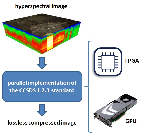
:Hyperspectral imaging is a technology which, by sensing hundreds of wavelengths per pixel, enables fine studies of the captured objects. This produces great amounts of data that require equally big storage, and compression with algorithms such as the Consultative Committee for Space Data Systems (CCSDS) 1.2.3 standard is a must. However, the speed of this lossless compression algorithm is not enough in some real-time scenarios if we use a single-core processor. This is where architectures such as Field Programmable Gate Arrays (FPGAs) and Graphics Processing Units (GPUs) can shine best. In this paper, we present both FPGA and OpenCL implementations of the CCSDS 1.2.3 algorithm. The proposed paralellization method has been implemented on the Virtex-7 XC7VX690T, Virtex-5 XQR5VFX130 and Virtex-4 XC2VFX60 FPGAs, and on the GT440 and GT610 GPUs, and tested using hyperspectral data from NASA’s Airborne Visible Infra-Red Imaging Spectrometer (AVIRIS). Both approaches fulfill our real-time requirements. This paper attempts to shed some light on the comparison between both approaches, including other works from existing literature, explaining the trade-offs of each one.

1. Introduction
Parallelization of different algorithms has been a hot topic in the last years [1]. As we are already at the limits of single-threaded applications [2], new programming paradigms are necessary to process the copious amounts of data we collect today.
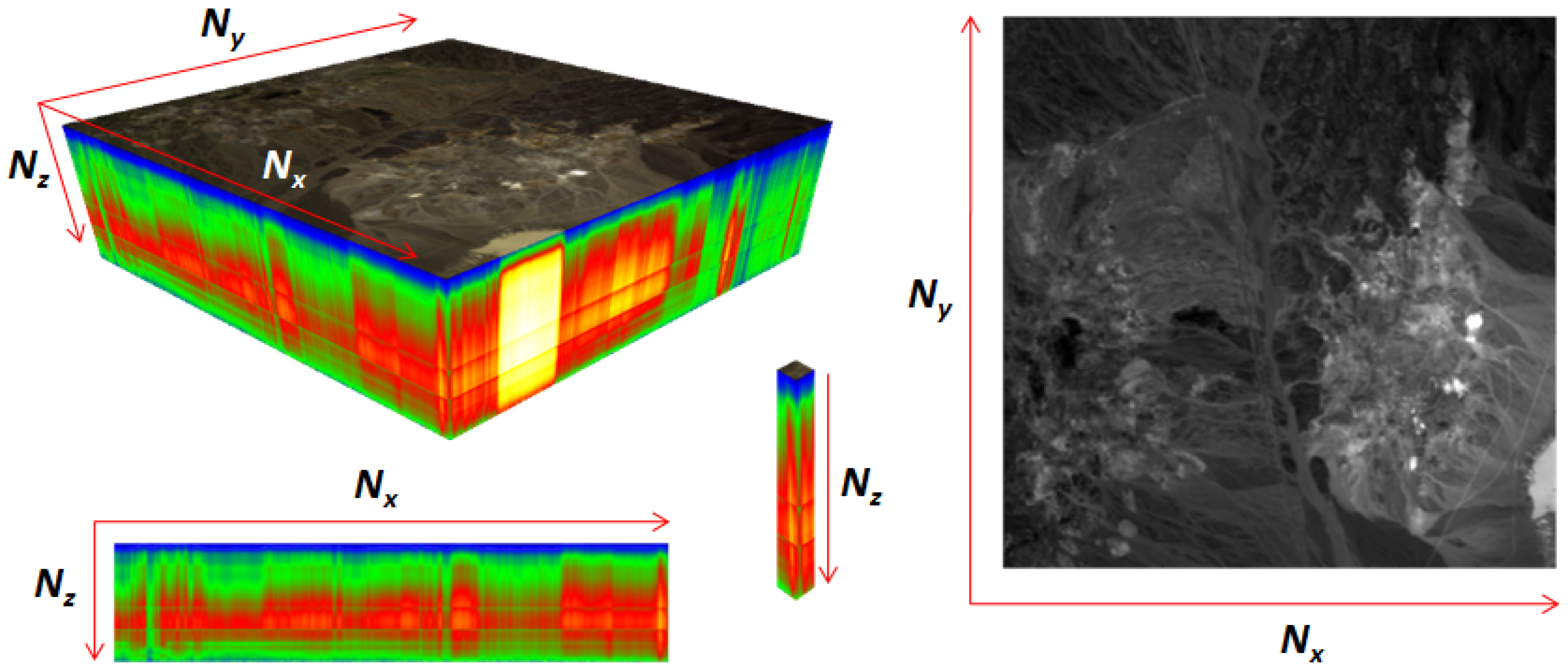
One of these data sources is hyperspectral imaging [3]. Building on the concept of capturing a mesh of pixels, this technology adds a third dimension by sweeping the electromagnetic spectrum, logging the intensity of hundreds of different wavelengths per pixel. This fact, along with the sensing resolution being quite above the 8-bit standard in normal images, boost the typical size of this images up to orders of GigaBytes.
Storing this massive amount of data in a compact manner is a must in order to save space, energy, and time. Compression algorithms can help ease this task by greatly reducing the information that needs to be stored. In an ideal scenario, we want our algorithms to perform in real time, giving the hyperspectral sensors the possibility of continuously collecting new data without running out of storage.
The interest for hyperspectral compression has been high in recent times. Some examples are Vector Quantization [4], using the vector-like nature of hyperspectral pixels; three dimensional wavelet compression [5], extending the concept used in two dimensional images; JPEG2000 adaptations [6], bringing the popular compression scheme to hyperspectral data, and much more [7]. All of these are very powerful but also computationally complex.
Linear prediction aims for a much more simple process, while having compression ratios on par or even better [8] than the mentioned algorithms. CCSDS 1.2.3 [9] is a realization of this concept. A low-complexity low-cost algorithm with the potential of being parallelized for real-time applications. For this particular algorithm, the CCSDS Green book standard [8] defines real-time as processing more than 20 MegaSamples per second (from now on MSa/s). We have also looked for the throughput of the fastest sensor and, to the best of our knowledge, found it to be the Airborne Visible InfraRed Imaging Spectrometer - Next Generation (AVIRIS-NG) [10] sensor, reaching 30.72 MSa/s. This is the threshold we have imposed on ourselves above which we will consider an implementation to be real-time.
Two of the platforms currently competing hand on hand to be the machines running parallel algorithms are FPGAs and GPUs. The former offers the flexibility of general purpose processors, and the performance of custom hardware. The latter, while not being as efficient, is readily available in almost every computer, and their ease of use overcomes their few disadvantages.
In this paper, we develop:
- A FPGA-based hardware version of the CCSDS 1.2.3 algorithm [9] for hyperspectral lossless compression. VHSIC (Very High Speed Integrated Circuits) Hardware Description Language (VHDL), a hardware definition language, has been used in this implementation. VHDL defines hardware components (such as memory, arithmetic and logic units, or custom circuits) and how they interconnect. This way, the specification can be mapped to different FPGA models by simply changing the target platform. FPGA implementations of this algorithm have already been presented in [11,12,13,14,15].In [11], they achieve a very simple and low occupancy implementation, by completely eliminating on board storage needs. This meant that, on each compression step, they needed to retrieve part of the image from memory, recalculating certain variables. This slowed down the algorithm enough that real-time compression was not possible for the newest sensors.All three [12,14,15] achieve real-time compression. However, they also use external RAM for intermediate storage, which introduces two downfalls in a spatial setting: the implementation needs more power to work, and it is more prone to errors since bit flips [16] in both the RAM and the FPGA can affect the output. Lastly, the implementation in [13] also needs external RAM, but only enough to hold one frame of the image. This avoids power consumption while still allowing a broad range of image dimensions to be compressed, but does not get around the bit flip problem.On our approach, we also strive for real-time compression. Taking advantage of the FPGAs on board memory, we use it as a buffer for the sensor’s output as well as for storing the variables needed for compression. This way, we only perform each calculation once and thus are able to achieve real-time compression, without the need for external RAM. This imposes limitations on the image frame size (See Figure 1) that can be processed, but not to the third dimension, which can grow indefinitely. Despite these limitations, we have not found a sensor with an image size too big for our algorithm when using the Virtex-7 board (Xilinx company, 2100 Logic Drive, San Jose, CA 95124-3400, USA) (see Table 2).
- An OpenCL software version of the same algorithm. OpenCL is a C/C++-based language that provides a framework for parallel computation across heterogeneous devices such as CPUs and GPUs. The code is device-independent, and a device-specific compiler makes the necessary adjustments for the code to run. By parallelizing to a higher degree than that of the FPGA, the GPU cores are able to also achieve real-time compression, using a combination of private and shared memory. The development time of this options is much lower than that of the FPGA. Even if this option has less throughput and is less power efficient than the first one, this alone can make up for it.GPU implementations of the CCSDS 1.2.3 algorithm [9] have already been presented in [17]. They develop two parallel implementations, using the OpenMP and Compute Unified Device Architecture (CUDA) languages, and test them on different configurations of CPU and GPUs. Their CUDA version significantly outperforms the OpenMP one, being targeted to more specific hardware. They surpass the real-time limit imposed by the newest sensors, attaining speeds faster than ours. However, they are using newer, more powerful GPUs, that double ours in cores and have faster core and memory clocks, making them use more power (from 75 W up to 150 W on their most powerful configuration compared with our 30 W requirement for real-time compression).
We compare both approaches, taking into account our findings as well as the existing literature, but do not draw a definitive winner. Each option has their strengths and weaknesses, and our goal is to provide a reference, for those looking to implement from scratch an algorithm, to see which platform might suit them best. We will gather results concerning power consumption, development times, and raw performance across a broad range of options.
The remainder of the paper is organized as follows. Section 2 presents an overview of the standard, focusing on a few key points that we will be taking advantage of. Section 3 describes its implementation on FPGA, with Section 4 doing the same for the GPU counterpart. Section 5 provides an experimental assessment of both power consumption and processing performance of the proposed algorithms, using well-known hyperspectral data sets collected by the NASA Jet Propulsion Laboratory’s AVIRIS [18] over the Cuprite mining district in Nevada, over the Jasper Ridge Biological Preserve in California and over the World Trade Center in New York. Finally, Section 6 concludes with some remarks and hints at plausible future research lines.
2. CCSDS 1.2.3 Algorithm
The CCSDS 1.2.3 [9] is a lossless compression algorithm for hyperspectral images. Hyperspectral images are made up of a number of bands , each containing a number of frames , which, in turn, host each pixels (see Figure 1).
A predictive model is generated per band, from which a prediction is made for each sample (Samples are denoted , where z represents the band (wavelenght) of the sample, y is the frame, and x the pixel within the frame. x and y are usually collapsed onto a single variable ). Its difference with the real value then encoded using prefix coding.
The basic flow of the algorithm is as follows:
- A sum of neighboring values of each sample is calculated as an estimate of four times the current sample. The standard defines two sum modes: neighbor-oriented and column-oriented, which vary in the number of neighboring samples used. Respectively:and
- A difference vector (Notation: We define , so we will either write for subscripting a variable ) is assembled from the differences between neighboring samples and the sum estimate. All differences follow the formula:If and we say the difference is central. When they differ, the pixel at will be either north, west or northwest of the one at . These are called directional differences ( for north, west and northwest). Differences from previous samples can also be added to this vector to improve performance, via the parameter P, indicating the number of previous central differences to be used.
- A weighted average of the differences is calculated where weights decide which of the differences is making a better prediction of the trend in sample values. A dot product is used here that multiplies the difference vector by the weigh vector .
- Weights are dynamically adapted to improve prediction accuracy based on the scaled prediction error which equals twice the difference between the predicted and the actual sample value.
- The difference between the actual sample value and predicted value, calculated from and , is sent to the encoder. The encoder works by encoding frequent and small values with few bits, using more bits for less frequent and bigger ones. The idea of using dynamic weights in the previous step is to minimize the values that the encoder receives as well as their differences.
- The encoder outputs a sequence of bits representing the compressed sample, using prefix coding so that we are able to later decode it without previously knowing each compressed sample’s length.
Data might come in one of three ways:
- Band Sequential (BSQ): Each band is processed one after another, and no pixels are completed until all the bands have been processed.
- Band Interleaved by Line (BIL): For each frame in the image, a full line (wavelength) is processed for each pixel before advancing to the next.
- Band Interleaved by Pixel (BIP): For each pixel in the image, all of its samples are processed in order before going to the next pixel.
Since each band has a different predictive model, parallelization of this algorithm resides in compressing multiple bands at once. The only ordering in which we can do that is BIP: as soon as a full pixel is received, we can compress it and proceed onto the next one. The compressed value only depends on the prediction state and the current sample, so a CCSDS core can be used at the same time for each of the samples in a pixel, accelerating by a factor of the number of bands the computation time. Each CCSDS core compresses one sample per cycle, interconnecting with other cores when intermediate results, such as differences, are shared.
However, full parallelization can not be achieved. Compressed samples vary in length, and they need to be tightly packed in the output stream, one after another. This imposes a limitation in our design, since gluing results together must be done serially. Luckily, as we will see, this serial part is quite fast. Segmenting the algorithm in parallel prediction and sequential encoding can therefore be quite beneficial.
3. FPGA Implementation of the CCSDS 1.2.3 Algorithm
Our approach to the implementation has four major stages that can be seen in Figure 2: first, a series of local operations (that is, their results only depend on input samples and not on previous results) are performed. Second, previous results are mixed with the local ones. Third, the prediction is made using adaptive weights. Lastly, it is is encoded, using an accumulator this time to improve performance.
In order to parallelize the algorithm, we must take the dependencies into account. On top of the BIP restriction, the combining part of the algorithm for a sample might depend (if ) of the differences generated by the local operations part of previous samples . We can solve this issue by simply cabling the results of one band’s local operations to multiple combiners. We also keep a difference buffer for when the whole pixel is not processed at once. The full circuit can be seen in Figure 3.
We now proceed to give a more detailed explanation:
Local operations: For this step, we need the current samples we are compressing, as well as neighboring values. These have already been processed since the algorithm works in a raster scan fashion. Given the prism-like nature of hyperspectral images, the required neighboring values have always been processed a fixed number of cycles ago. These are shown for BIP mode in Table 1.
This fact suggests the viability of using a First In First Out (FIFO) queue to store previous samples. Its size needs to be that of the longest distance among samples. We also observe that multiple values from the queue need to be read in the case of neighbor-oriented sums. This can be solved by having a multi-read queue, or by chaining queues of the partial distances between samples. We opt for the second option, since it is cheaper in hardware utilization. An example of that chaining can be seen on Figure 4.
Combining: When the number of previous bands used for prediction , we need the central local difference from the P previous bands in the combining step. This presents the next challenge: that difference might be being calculated by another copy of the algorithm, or has just been calculated in the previous cycle. In the first case, we can just send the result directly from the difference generator to the difference filter that needs it. In the second case, a buffer records the differences needed from previous cycles, and is able to deliver them when needed, as seen in Figure 3.
Prediction: A weighted average of the combined differences is added to the local sum to make a prediction of the current sample, which is then mapped to a positive integer and sent to the encoder. Weights are dynamically updated to improve the next sample’s prediction, adjusting for the error yielded by the current one.
These weights are needed per band, as each one follows a different model. Usually, the parallelization degree C is lower than the image’s number of bands , so storing these weights in a register is not viable since they would be overwritten with each step. To solve this, each CCSDS core is assigned certain bands , …, which it will process for every pixel. It also has a FIFO queue in which to store all of the (rounded up) weights. In some cases, this might result in some CCSDS cores being idle if the division is not exact. It is advised that C divides exactly , so as to not lose performance.
Encoding: Finally, the differences from the previous step and the real values are encoded using Run-Length Encodings [19]. An accumulator in this step behaves much as the prediction’s weights, and one is kept per band in the same fashion. A sequential counter is used to periodically update it, but instead of buffering it, we calculate it on the fly based on the current image coordinates. This counter is fed to all CCSDS cores at the same time, since its value is shared between all of them.
After all the parallel work is done, the results need to be serialized again because ordering of compressed samples is crucial in the output file. A special module is responsible for taking all the simultaneously compressed samples, and sending them to the output following the same order in which they came into the compressor.
4. OpenCL Implementation
There are many ways of programming parallel devices, but one of the most portable is OpenCL. It allows us to define how the device behaves, and the compiler has the task of deciding how that maps to its internal structure.
Following the same ideas we used for the FPGA implementation, we now develop a OpenCL code capable of compressing in parallel a hyperspectral image given in BIP ordering. As with FPGAs, we can decide how many threads collaborate to compress the image, having a limit imposed by the nature of the algorithm at threads.
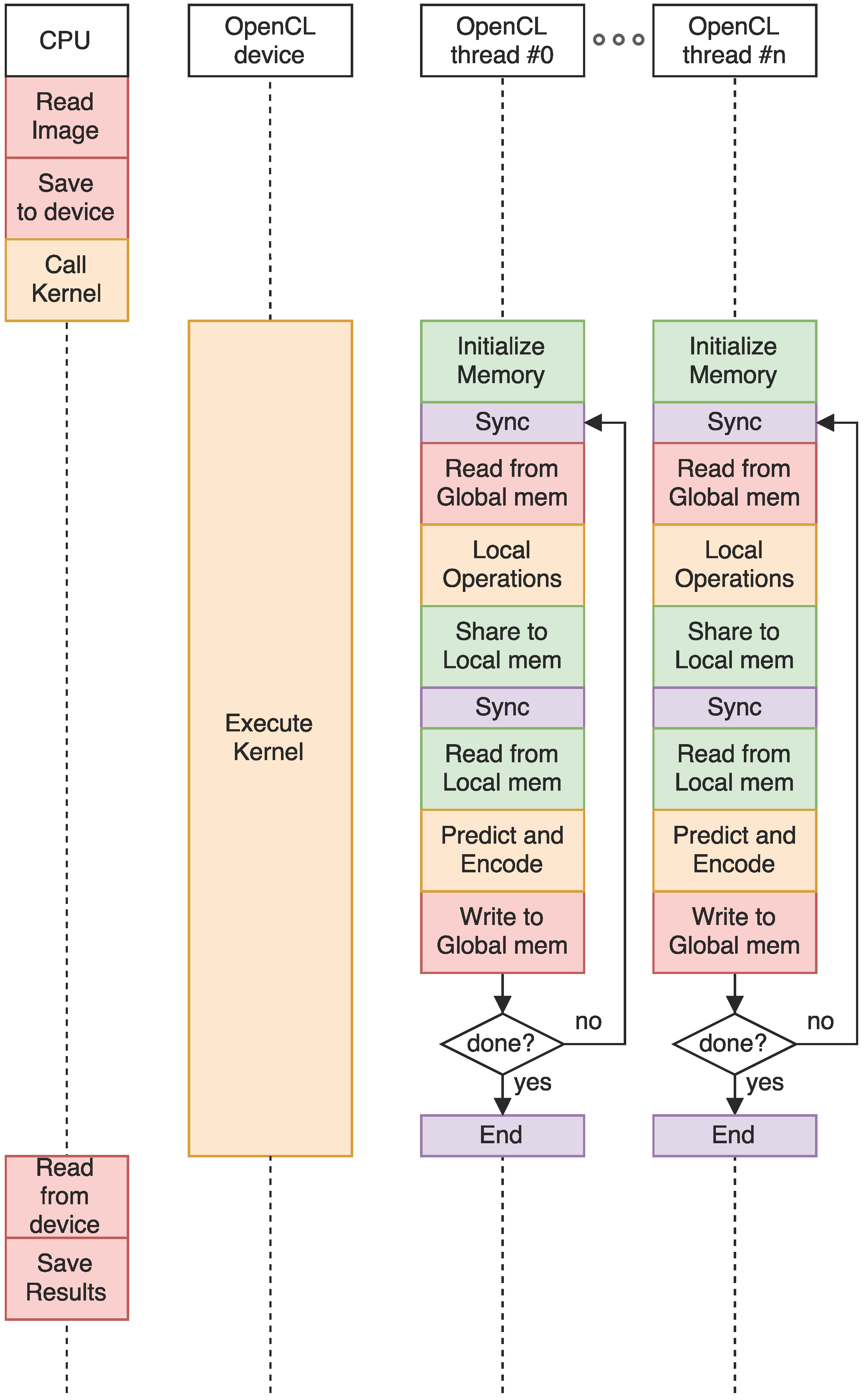
The timeline of the execution of the OpenCL code can be seen on Figure 5.
First, the CPU receives the image from the imaging device, and copies it to the device’s global memory. Then, the OpenCL kernel is called. The device will set up the threads and memory automatically, following our instructions in how many threads and memory it needs. After the set up, code execution starts. Each of our threads initializes variables such as the weight vectors or accumulators. After that, it starts compressing samples:
- The threads are synced to ensure local memory reads are all done before it can be modified.
- Local operations are done and saved to local memory, where they are shared between threads. Namely, the central local difference is shared.
- Threads are again synced so that the local memory is fully updated before being read by the other threads.
- These shared results are read from local memory, prediction and encoding are done, and the results are saved to global memory.
- This process is repeated until the image is fully processed. Each thread compresses exactly one sample per cycle.
After the kernel is executed, the CPU reads the results from the device, and is then used to pack the parallel results into the final compressed file.
5. Experimental Results
In this section, we study the performance (measured in MegaSamples per second (MSa/s)) of both the FPGA and OpenCL versions of the algorithm using a variety of different devices. We also compare power consumption, time it took to develop both versions, and other capabilities of both approaches. This is what will set them apart, since these parameters will vary wildly, and trade-offs will have to be made when choosing one or the other.
The data used from testing comes from real images. The real images are the well-known Jasper Ridge (JR), World Trade Center (WTC), and Cuprite (CPR) from the AVIRIS sensor. All three are used for testing new algorithms on hyperspectral images. The compression results have been validated using the software Empordá [20] and European Space Agency (ESA)’s implementation [21].
The algorithm parameters are defaulted to those given in [8] unless otherwise explicitly stated. Since image size affects algorithm performance (and occupancy in the case of the FPGA version), we assume an image of size , one of AVIRIS’s resolutions. We also introduce a new parameter, C, which is the number of samples that are compressed at the same time, or degree of parallelism. R, the register size for the compressor arithmetic operations, is set to the minimum value that does not produce overflow as per [8].
The reference speed above which we consider real-time to be achieved is that maximum speed at which an AVIRIS-NG sensor can deliver data: 30.72 MSa/s [10]. We also assume a bit depth of 16 b, the maximum allowed by the standard, so that our results serve as a reference for a worst case scenario performance, which can only be improved when restricting the parameters.
5.1. FPGA Implementation Results
For the FPGA implementation, the modules have been written in VHDL. Xilinx ISE (Xilinx company, 2100 Logic Drive, San Jose, CA 95124-3400, USA) has been used to tie everything together and synthesize the circuits for both the Virtex-4 XC2VFX60 FPGA (Xilinx company, 2100 Logic Drive, San Jose, CA 95124-3400, USA) (equivalent to space-grade Virtex-4QV XQR4VFX60 FPGA) and the powerful Virtex-7 XC7VX690T. We have also gathered synthesis results for the Virtex-5 XQR5VFX130, the latest most powerful space-qualified FPGA, as it serves as a theoretical limit for what could be achieved with this design on space.
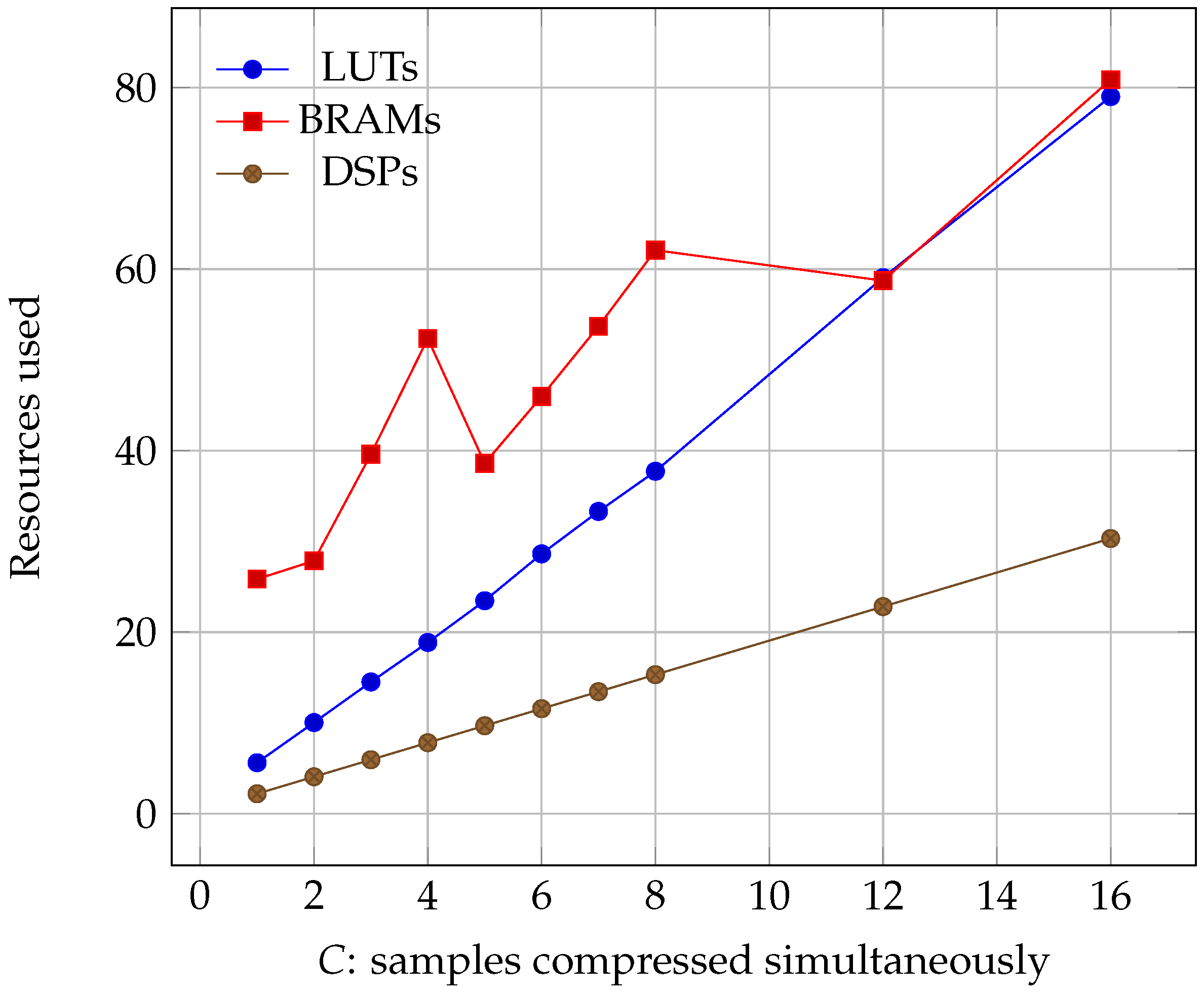
Regarding occupancy, we can see the results for all of the three boards in Figure 6, Figure 7 and Figure 8. We see that all three parameters: Lookup Tables (LUTs), Block Random Access Memories (BRAMs), and Digital Signal Processors (DSPs) grow linearly with C. However, it must be noted that, while LUT and DSP requirements do increase, the memory needed only depends on the size of the image. Its growth is a consequence of the algorithm needing to read more information at the same time, which can only be accomplished by using more BRAMs.
Table 2 shows the different resources needed for the Virtex-7, setting , for the sizes of images that different sensors output. By design, does not affect the size at all, so increasing image resolution in this axis would be the ideal choice. and do affect it, with having more impact since it not only affects the memory needed for buffering samples, but also the memory needed for weight and accumulator storage. This can be seen by, for example, comparing M3-Global and IASI [8], with the former using 10 times more memory despite the final image being 50 times smaller, all because M3-Global has a big against the big of IASI.
Another important aspect of the algorithm is speed. We can see a diagram of the algorithm pipeline, along with maximum speeds, in Figure 9. We see that, when using the default clock on a Virtex-4, our design is capable of beating the reference speed with a 30% increase in speed. If we push it to its limits, the slowest component (and thus the limiting factor of the system) clocks in at around 116 MSa/s, or a 286% increase over the reference speed. Moreover, synthesis clock results show, for , a 54.9% speed increase for the Virtex-5, and a 89.1% increase for the Virtex-7, which would put them, respectively, at 179.7 MSa/s and 219.4 MSa/s. These values were taken using the same synthesis options used for the Virtex-4 synthesis, which are Xilinx Project Navigator 14.7’s defaults.
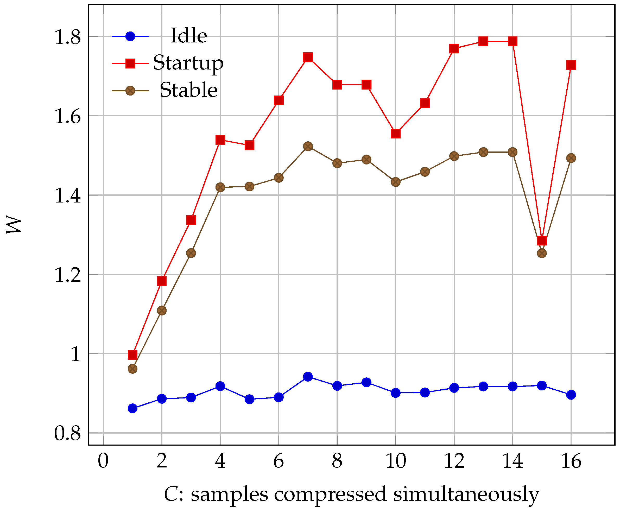
A question that might arise is what the point of massive parallelization is. Real-time compression is achieved with in a Virtex-4 with the default 100 Mhz clock. In addition, there are some serial parts of our algorithm that can not be sped up by increasing C, so we would be adding unnecessary hardware. However, when we take a look at the power consumption in Figure 10, we see that it does not keep increasing when we add more CCSDS cores. In fact, given the board’s characteristics, there is a huge dip in consumption at C = 15, meaning that, if our aim is to save on power, we need to use more FPGA area so that clock speed is lowered for the CCSDS cores.
In order to measure power consumption, we used the USB Interface Adapter EVM [22] (TEXAS instrument, 12500 T I Blvd, Dallas, TX 75243, USA). This device allows us to probe the Virtex-7’s PMBus (Power Management Bus) and read power related values, such as voltage and amperage from the board. We can log power consumption to a comma-separated values (CSV) file, and then analyze it to see what the sustained values are, getting an exact measurement better than that from simulation tools. The PMBus is not available for the Virtex-4 and 5 devices that we have tested. For these cases, Xilinx’s Power Estimation tool (XPE) [23] has been used. After implementing the design, a summary of the required resources is input into XPE, as well as the expected toggle rates, which we have left by default. XPE then returns an estimate of the design’s power consumption. These results are later discussed in Table 3.
Changing our variable C only changes the CCSDS module, and all the others remain the same. For , the bottleneck is the algorithm, and it is not fast enough to process all the samples, so it is always working at maximum load. When , the bottleneck shifts to the mixer module. This means that now the cores can work at a lower clock speed, while still maintaining the same throughput. This lower speed means that more time is available to dissipate the heat, and cooler temperatures mean a more efficient energy use. Thus, even if we increase the total footprint, we can in some cases decrease the total consumption. Of course, as evidenced by the graph, this behaviour depends on the synthesis and implementation tools, and how they decide to place our components. For best results, we should test our circuit with different degrees of parallelization, and see which one suits our needs the best.
5.2. OpenCL Implementation Results
For the OpenCL implementation, a kernel code has been written in OpenCL for the OpenCL devices, along with a wrapper in C++ for the CPU to control it. Parameter values are the same as in the FPGA implementation to keep a fair competition.
The beautiful thing about OpenCL is that we can compile it for many devices, and quickly check which ones deliver sufficient performance. We use two different GPUs and a CPU for testing:
- Nvidia GT440 (NVIDIA company, 2701 San Tomas Expy, Santa Clara, CA 95050, USA): It has 96 cores clocked at 810 MHz, with 1 GB of memory having 28.8 GB/s of bandwidth. Thermal design power (TDP) is 65 W.
- Nvidia GT610: It has 48 cores clocked at 810 MHz, with 1 GB of memory having 14.4 GB/s of bandwidth. TDP is 29 W.
- Intel i7-6700 (Intel company, 2200 Mission College Blvd, Santa Clara, CA 95054-1549, USA): IT has eight cores clocked at 3.4–4 GHz, with 8 GB of memory. TDP is 65 W.
Both GPUs are used along with the Intel i7-6700 CPU, which will interface with them, sending data and gathering results. It also doubles as an OpenCL device using its built-in parallel processing, although its performance is lower than that of the GPU.
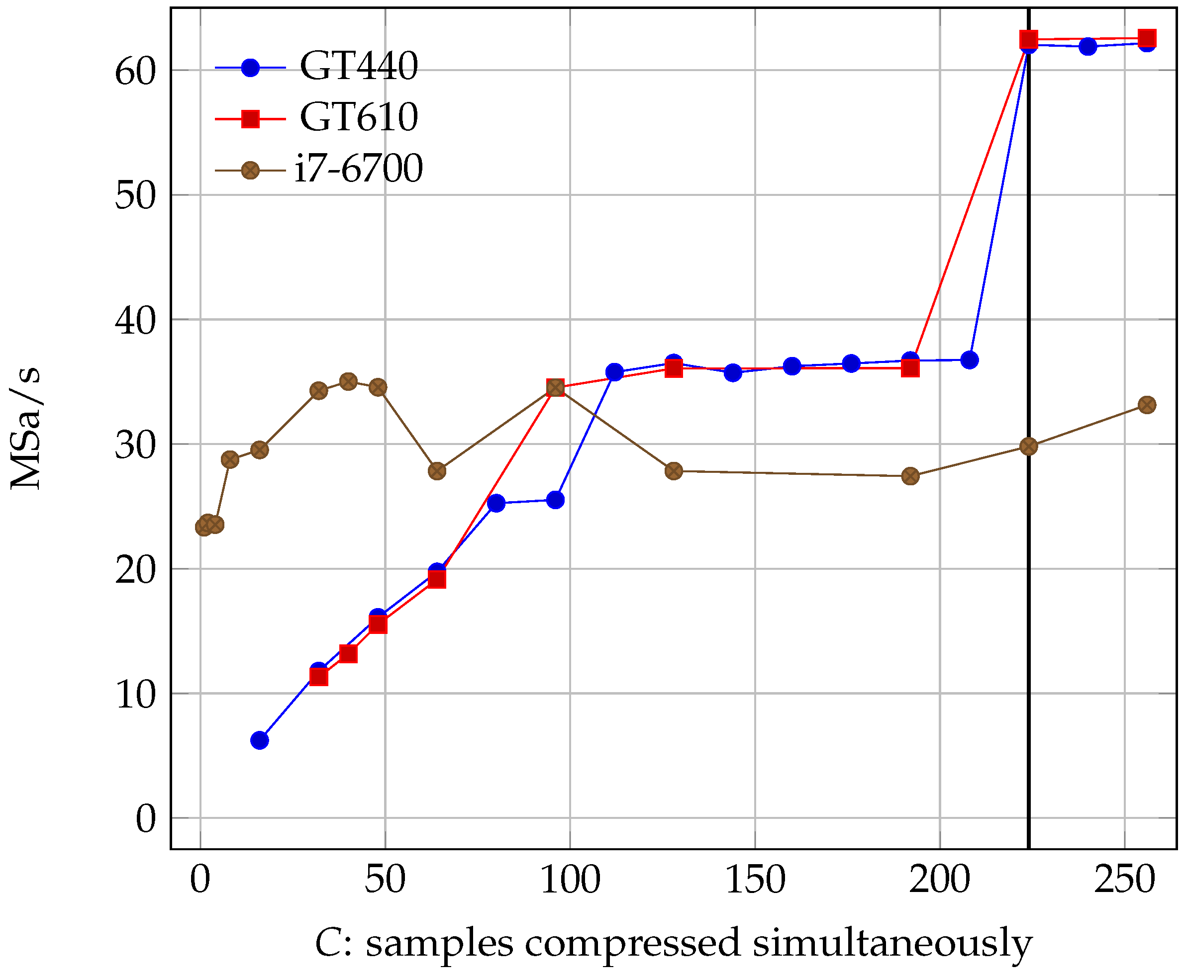
As with the FPGA counterpart, this implementation has a serial part that can not be parallelized, specifically assembling the compressed samples in the bit stream that forms the output. As each compressed sample varies in length, we do not know in advance where it will lay on the output stream, and thus can not add it until the previous has been put in place. Fortunately, this part of the code is quite fast and the parallel part is still the bottleneck until we get to a quite high parallelization. We can see the effect of varying the number of bands, C, for the kernel in Figure 11.
GPU speed increases almost linearly with the number of threads (albeit in steps and not smoothly); however, CPU speed is very erratic for this particular model. The GPU performance stops increasing when the number of threads surpasses the number of bands in the image (recall that the maximum number of useful threads we can have is limited by the number of bands ), so if we want the maximum speed possible we need to parallelize as much as the GPU allows us up to the band limit.
The C++ wrapper that later processes the data output by the OpenCL device had, throughout our tests, a minimum speed of 84.19 MSa/s. The maximum speed achieved by the GPU was 62.56 MSa/s with , and we can safely say that the serial part of the algorithm, which is not done on the GPU, is not a bottleneck. Comparing these results with the reference speed, we observe a 103.64% increase in speed, giving us a big margin for the improvement of sensors before we need to reevaluate the design.
One of the drawbacks with our OpenCL approach is that the image has to be fully loaded on the OpenCL device’s memory. In our tests, this was not a problem, as all of the tested devices could store the MB, plus another 422.5 MB for the outputs, for a total of 563.3 MB of data. This could be improved by partially loading the image and unloading the results, but it should be noted that doing multiple memory transfers would be slower than doing only one.
5.3. Comparison
We have studied both approaches individually, but the most interesting part is seeing how they fare when facing each other. Studying the differences with this particular algorithm, CCSDS 1.2.3, is interesting because of the broad range of implementations already in the literature, which offer multiple viewpoints of the same problem. Implementations of similar new algorithms might benefit from the particularities of one or the other. We present this comparison as a guide to help decide which platform (FPGA or GPU) to use for these new developments. Table 3 shows these results in more detail:
The first thing we are interested in is development times. For this, we only have our times, since the existing literature does not comment on this detail. Our algorithms have been developed with a similar background in both VHDL and OpenCL coding, so times should not be skewed. Both take into account writing the code, as well as debugging and testing it.
Our FPGA version took around three man-months to develop. Testing, fixing errors, and generally programming in VHDL is much harder than OpenCL, since the bugs now come from both a software and a hardware standpoint. Despite all of this, we get a really refined product, tailored at the logic gate level for this specific algorithm. Conversely, the OpenCL version was completed within two man-weeks. This six-fold increase can not be explained by a difference in coding experience, and we believe it to be the general case given the similarity between GPU programming languages and traditional imperative languages, which users are generally more familiar with.
The next interesting thing to consider is raw speed. Sometimes, we just need algorithms to perform fast, regardless of other factors such as power consumption. In this case, GPUs take the cake with Hopson et al.’s [17] CUDA version achieving 329.2 MSa/s, 50% faster than our fastest FPGA version. In this case, the bottleneck in the FPGA version was the serial part of the algorithm, where packing the variable-length codewords into the output stream limited performance. Hopson et al. solved this issue by cleverly precalculating the boundaries of the codewords, logically ORing the 4-byte words where different segments met. This could be done in parallel, so they took full advantage of the GPU. Applying a similar strategy for the FPGA version would certainly improve its rates, but would imply losing its independency from external memory.
Looking at power consumption, we clearly see that the winners are FPGAs. Not only are they less power demanding, but they are more than an order of magnitude more efficient at using that power. The limit is set at 122.60 MSa/s/W with our Virtex-4 version (based on XPE estimations). Ignoring estimations, Keymeulen et al.’s [14] version, at 57.10 MSa/s/W, is the most efficient one. In any case, both significantly outperform the most efficient GPU version, at 3.96 MSa/s/W. One thing we can take away from this, though, is that the more modern GPUs are increasingly more efficient, since the GTX 560 M is four times as efficient as the GT 440.
Other aspects that we can not directly compare are:
- Some FPGAs (in this comparison the Virtex-5QV) are radiation-hardened and could be used in a spatial setting, which, for this algorithm, is particularly interesting since hyperspectral images can be taken from satellites.
- The FPGA version can run by itself, connecting directly to the sensor and/or memory. The GPU version needs a processor to help it along.
- GPUs are readily available in almost every computer, so the trouble of getting an FPGA might not be worth it for some.
- The speed of FPGAs does not depend on external factors, such as interruptions by system calls that can occur on a GPU managed by an OS. For a real-time setting where failures can not be tolerated, this might be an important issue.
- Some GPU codes such as OpenCL, and directive-based programming such as OpenMP, run on CPUs. However, they are neither faster nor more efficient than either FPGAs or GPUs. However, this can be very useful for testing when specific hardware is not available.
Despite their pros and cons, both alternatives met and exceeded the real-time expectations, and both can be further improved. GPUs are limited mostly by parallelization, since they easily achieve the maximum possible (parallelization equal to the number of bands), and would improve their performance with more threads being launched. FPGAs are limited by the serial part of the algorithm, since the parallel part outperforms GPUs for the same value of C. The older models such as the Virtex-5 (space qualified) also suffer from a lack of resources, since the circuit can not fit for large values of C, or when dealing with very large images.
6. Conclusions
We developed a VHDL implementation of the CCSDS 1.2.3 standard for compressing hyperspectral images, suitable for synthesis on FPGAs, along with an OpenCL version of the same algorithm, suitable for execution on any OpenCL device such as CPUs, GPUs or even some FPGAs as well. We compared them with existing implementations for both FPGAs and GPUs.
Results show that both options have many advantages and disadvantages. In the case of needing reliability and low power consumption, FPGAs are the obvious choice. Some even are radiation-hardened for usage in space, from where many hyperspectral images are captured. GPUs are best for obtaining results faster. Testing is easier, and integration with other parts or algorithms is also quicker. Further testing with other types of parallel algorithms will help clarify if the differences observed here are applicable outside of a hyperspectral setting, which we believe is entirely possible.
All in all, we can not just guess what the best platform for improving an algorithm’s performance is. We need to know what the advantages of each system are, and choose the one that better fits our needs. Future research studying these implementations for other algorithms might shed more light in this open debate between FPGAs and other non re-programmable devices.
Acknowledgments
This work has been supported by the by the Spanish Ministry of Science and Innovation under reference READAR (TIN2013-40968-P).
Author Contributions
D.B. design a parallel implementation of the algorithm; C.G. and D.M. conceived and designed the experiments; D.B. performed the experiments; D.B., C.G. and D.M. analyzed the data; D.B., C.G. and D.M. wrote the paper.
Conflicts of Interest
The authors declare no conflict of interest.
References
- Leighton, F.T. Introduction to Parallel Algorithms and Architectures: Arrays Trees Hypercubes; Elsevier: Amsterdam, The Netherland, 2014. [Google Scholar]
- Sutter, H. The free lunch is over: A fundamental turn toward concurrency in software. Dr. Dobb’s J. 2005, 30, 202–210. [Google Scholar]
- Chang, C.-I. Hyperspectral Imaging: Techniques for Spectral Detection and Classification; Springer: Baltimore, MD, USA, 2003; Volume 1. [Google Scholar]
- Ryan, M.J.; John, F.A. The lossless compression of AVIRIS images by vector quantization. IEEE Trans. Geosci. Remote Sens. 1997, 35, 546–550. [Google Scholar] [CrossRef]
- Dragotti, P.L.; Poggi, G.; Ragozini, A.R. Compression of multispectral images by three-dimensional SPIHT algorithm. IEEE Trans. Geosci. Remote Sens. 2000, 38, 416–428. [Google Scholar] [CrossRef]
- Penna, B.; Tillo, T.; Magli, E.; Olmo, G. Progressive 3-D coding of hyperspectral images based on JPEG 2000. IEEE Geosci. Remote Sens. Lett. 2006, 3, 125–129. [Google Scholar] [CrossRef]
- Motta, G.; Rizzo, F.; Storer, J.A. (Eds.) Hyperspectral Data Compression; Springer: New York, NY, USA, 2006. [Google Scholar]
- Lossless Multispectral & Hyperspectral Image Compression. CCSDS 120.2-G-1. 2015. Available online: https://public.ccsds.org/Pubs/120x2g1.pdf (accessed on 19 September 2017).
- Lossless Multispectral & Hyperspectral Image Compression. CCSDS 123.0-B-1. 2012. Available online: https://public.ccsds.org/Pubs/123x0b1ec1.pdf (accessed on 19 September 2017).
- AVIRIS-NG Website. Available online: https://aviris-ng.jpl.nasa.gov/ (accessed on 19 September 2017).
- Santos, L.; Berrojo, L.; Moreno, J.; López, J.F.; Sarmiento, R. Multispectral and Hyperspectral Lossless Compressor for Space Applications (HyLoC): A Low-Complexity FPGA Implementation of the CCSDS 1.2.3 Standard. IEEE J. Sel. Top. Appl. Earth Obs. Remote Sens. 2016, 9, 757–770. [Google Scholar] [CrossRef]
- Keymeulen, D.; Luong, H.; Pham, T.; Ghossemi, H.; Shin, S.; Kiely, A.; Klimesh, M.; Cheng, M.; Dolman, D.; Holyoake, C.; et al. FPGA Implementation of Space-Based Lossless and Lossy Multispectral and Hyperspectral Image Compression. In Proceedings of the 5th International Workshop on On-Board Payload Data Compression, Frascati, Italy, 28–29 September 2016. [Google Scholar]
- Theodorou, G.; Kranitis, N.; Tsigkanos, A.; Paschalis, A. High Performance CCSDS 123.0-B-1 Multispectral & Hyperspectral Image Compression Implementation on a Space-Grade SRAM FPGA. In Proceedings of the 5th International Workshop on On-Board Payload Data Compression, Frascati, Italy, 28–29 September 2016. [Google Scholar]
- Keymeulen, D.; Aranki, N.; Bakhshi, A.; Luong, H.; Sarture, C.; Dolman, D. Airborne demonstration of FPGA implementation of Fast Lossless hyperspectral data compression system. In Proceedings of the 2014 NASA/ESA Conference on Adaptive Hardware and Systems (AHS), Leicester, UK, 14–17 July 2014. [Google Scholar]
- Lopez, G.; Napoli, E.; Strollo, A.G. FPGA implementation of the CCSDS-123.0-B-1 lossless Hyperspectral Image compression algorithm prediction stage. In Proceedings of the 2015 IEEE 6th Latin American Symposium on Circuits & Systems (LASCAS), Montevideo, Uruguay, 24–27 February 2015. [Google Scholar]
- Serrano, F.; Clemente, J.A.; Mecha, H. A Methodology to Emulate Single Event Upsets in Flip-Flops using FPGAs through Partial Reconfiguration and Instrumentation. IEEE Trans. Nucl. Sci. 2015, 62, 1617–1624. [Google Scholar] [CrossRef]
- Hopson, B.; Benkrid, K.; Keymeulen, D.; Aranki, N. Real-time CCSDS lossless adaptive hyperspectral image compression on parallel GPGPU & multicore processor systems. In Proceedings of the 2012 NASA/ESA Conference on Adaptive Hardware and Systems (AHS), Erlangen, Germany, 25–28 June 2012; pp. 107–114. [Google Scholar]
- AVIRIS Website. Available online: https://aviris.jpl.nasa.gov/aviris/instrument.html (accessed on 19 September 2017).
- Golomb, S.W. Run-length encodings. IEEE Trans. Inf. Theory 1966, 12, 399–401. Available online: http://urchin.earth.li/~twic/Golombs_Original_Paper/ (accessed on 19 September 2017). [CrossRef]
- GICI Group, Empordá Software, Universitat Autonoma de Barcelona, 2011. Available online: http://www.gici.uab.es (accessed on 19 September 2017).
- Luca Fossati, Lossless Ccsds. European Space Agency, 2011. Available online: https://amstel.estec.esa.int/tecedm/misc/ESA_OSS_license.html (accessed on 19 September 2017).
- Texas Instruments’s USB Interface Adapter EVM. Available online: http://www.ti.com/tool/usb-to-gpio (accessed on 19 September 2017).
- Xilinx Power Estimator. Xilinx. Available online: https://www.xilinx.com/products/technology/power/xpe.html (accessed on 19 September 2017).
Figure 1.
On the top left, a representation of a hyperspectral image. On the right, a band of the image, showing the intensity of a specific wavelength. On the bottom left, a frame of the image. In the bottom center, a pixel, containing all the wavelengths that conform it. The image is Cuprite from NASA’s Jet Propulsion Laboratory.

Figure 2.
FPGA implementation of the CCSDS 1.2.3 algorithm.
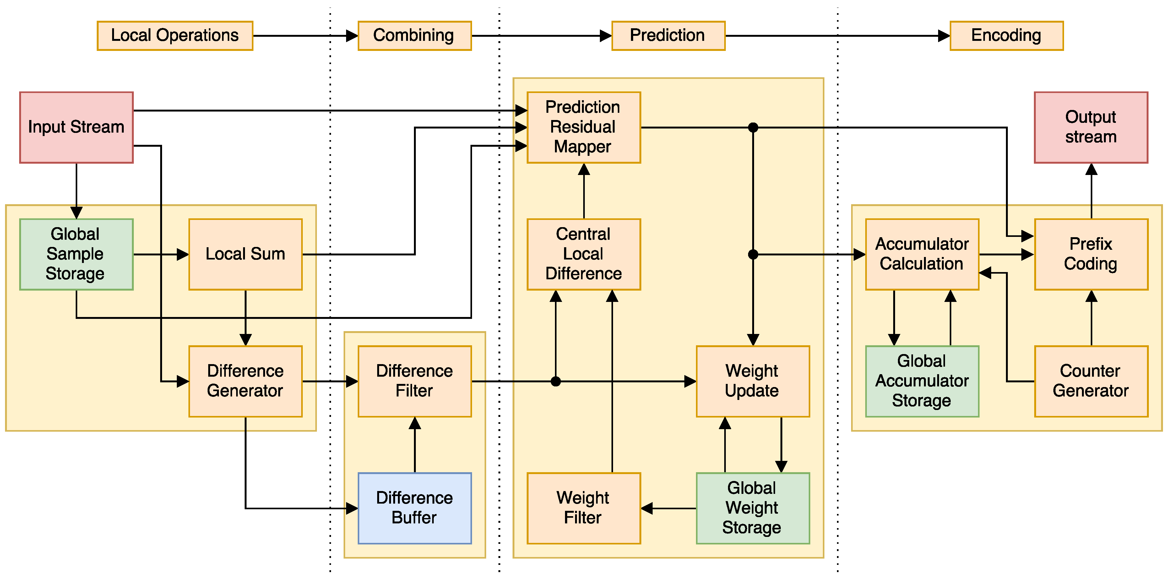
Figure 3.
Parallel FPGA implementation of the CCSDS 1.2.3 algorithm.
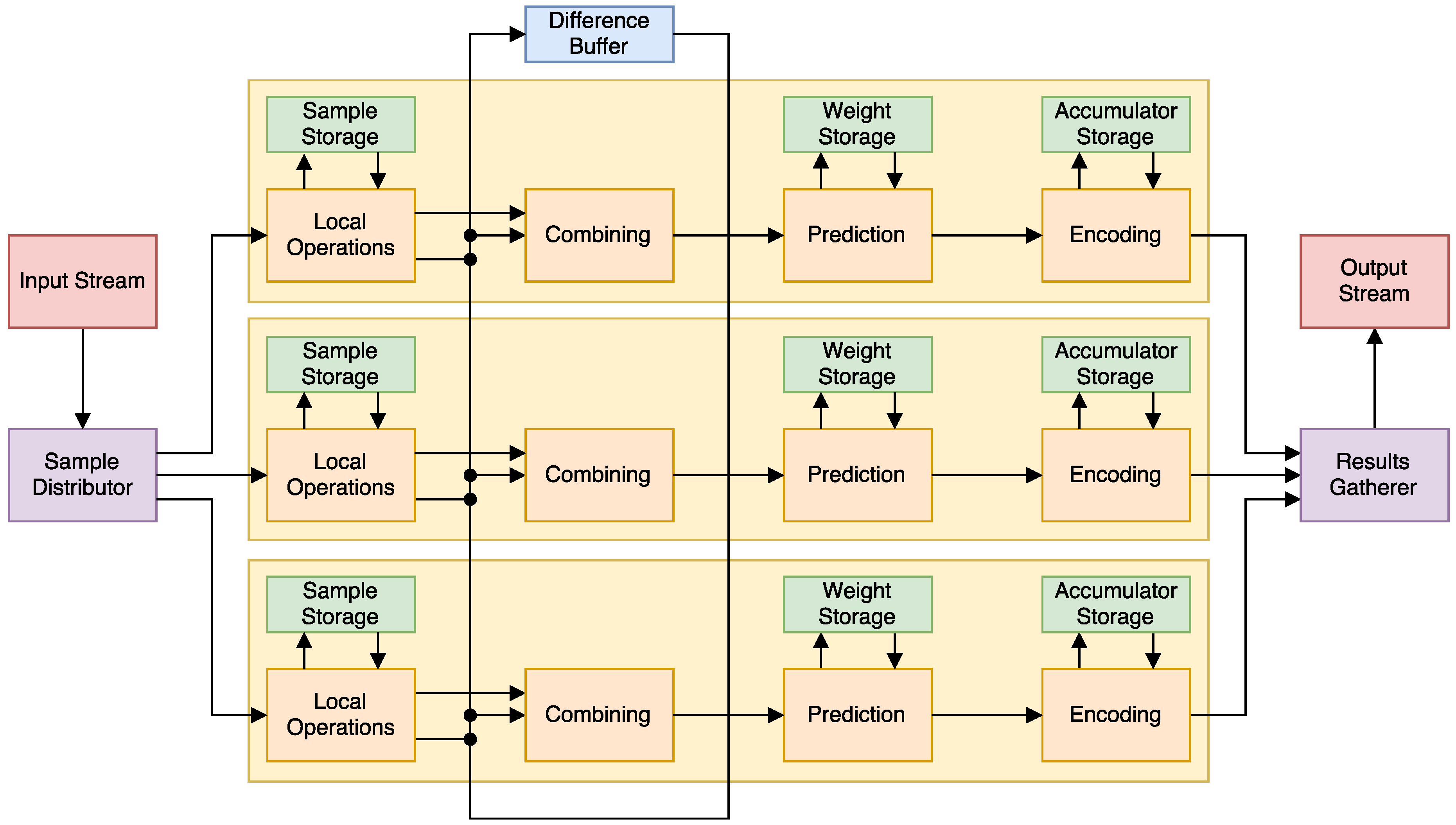
Figure 4.
Queue chaining for Band Interleaved by Pixel (BIP) scan. Red is the current sample, and the rest of colors are different queues feeding into each other. The neighborhood is assembled from the first element of each queue.
Figure 4.
Queue chaining for Band Interleaved by Pixel (BIP) scan. Red is the current sample, and the rest of colors are different queues feeding into each other. The neighborhood is assembled from the first element of each queue.
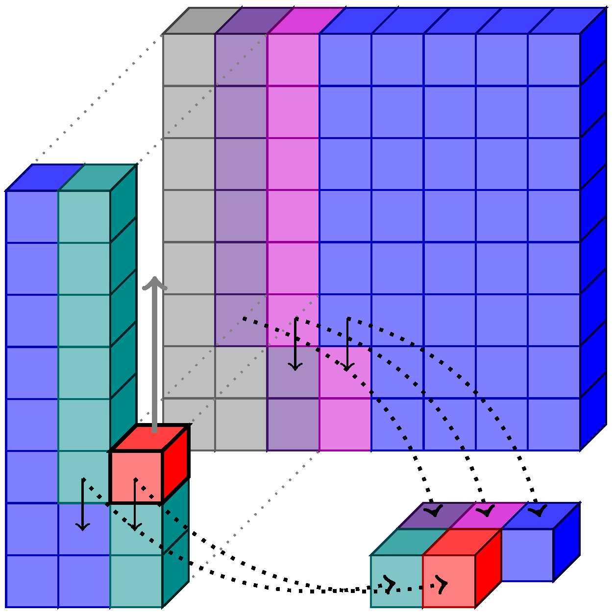
Figure 5.
OpenCL implementation timeline.

Figure 6.
Percentage of the Virtex-4 resources used as the number of samples compressed simultaneously increased (lower is better).
Figure 6.
Percentage of the Virtex-4 resources used as the number of samples compressed simultaneously increased (lower is better).
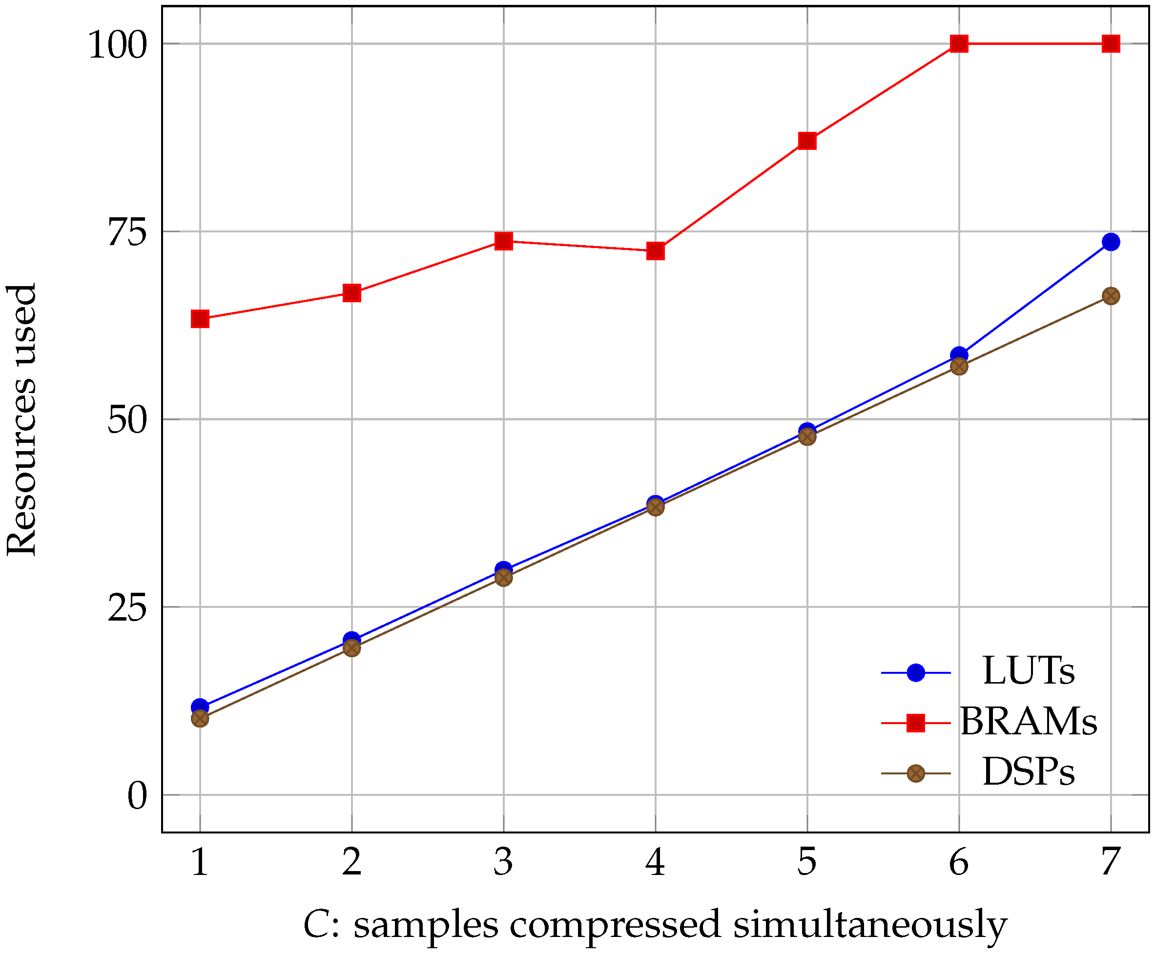
Figure 7.
Percentage of the Virtex-5 resources used as the number of samples compressed simultaneously increased (lower is better).
Figure 7.
Percentage of the Virtex-5 resources used as the number of samples compressed simultaneously increased (lower is better).

Figure 8.
Percentage of the Virtex-7 resources used as the number of samples compressed simultaneously increased (lower is better).
Figure 8.
Percentage of the Virtex-7 resources used as the number of samples compressed simultaneously increased (lower is better).
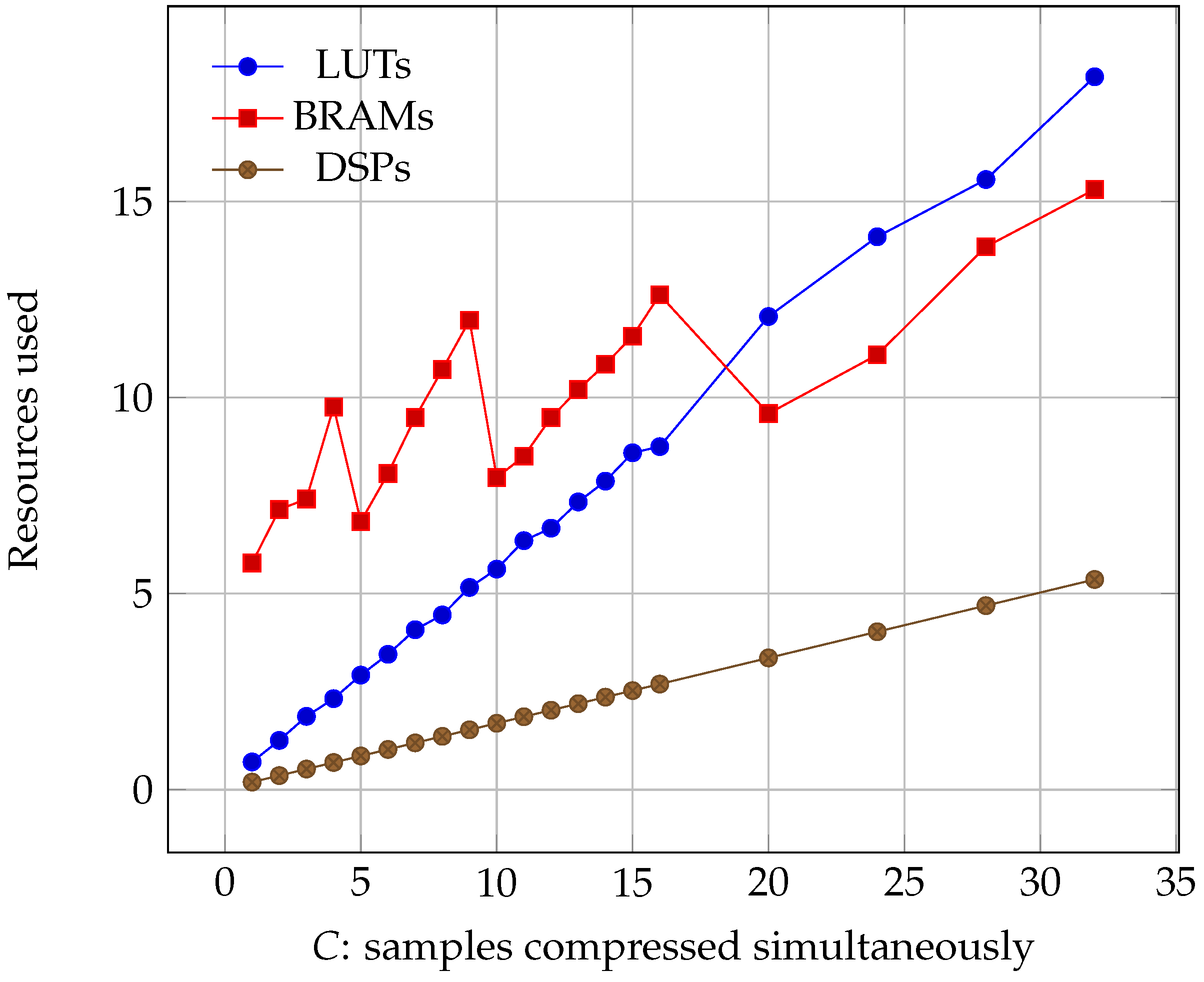
Figure 9.
Speed of the different pipelined components on the Virtex-4 board when .
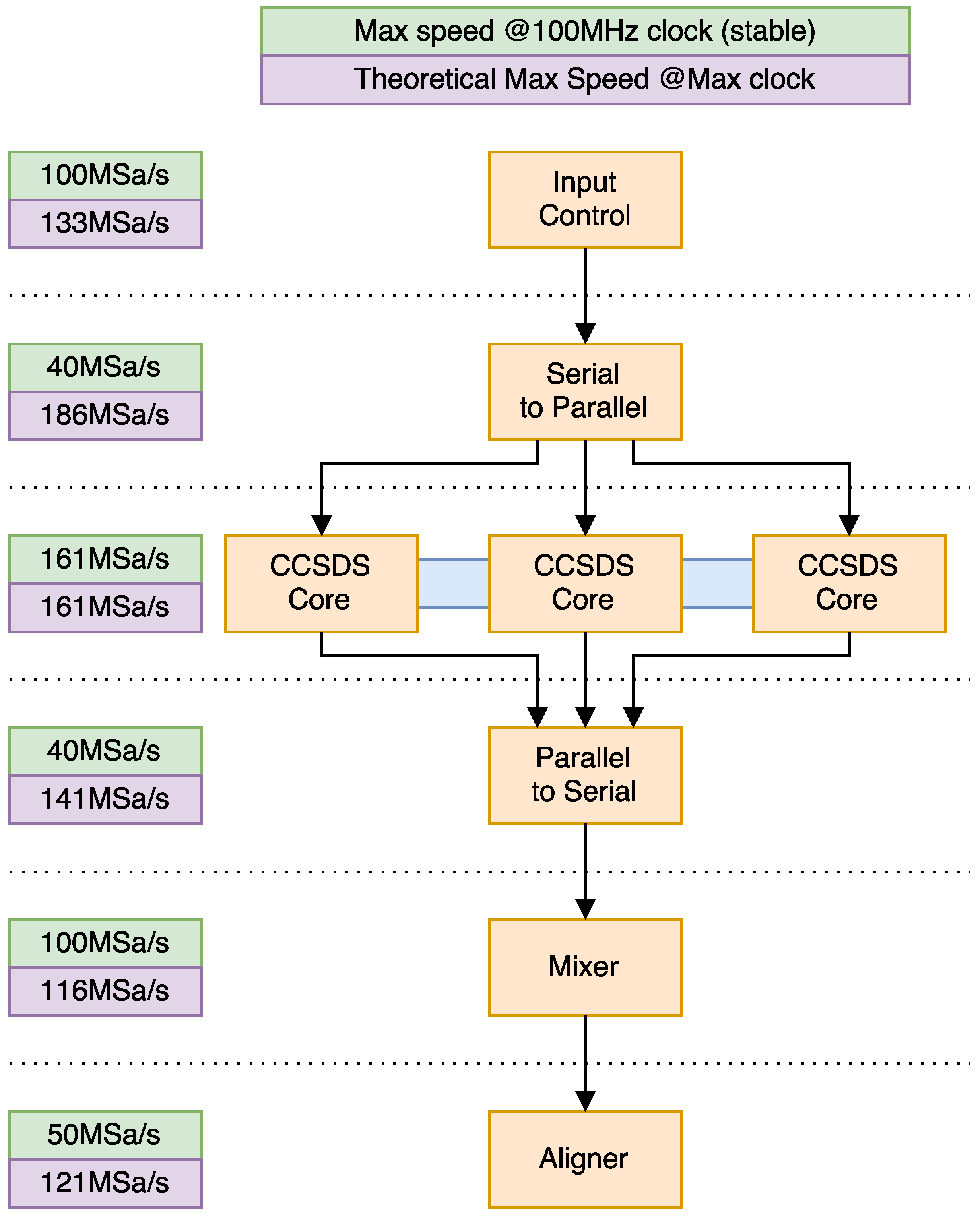
Figure 10.
Virtex-7 power consumption as the number of simultaneously compressed samples increases. Note the stalling after when the design has reached real-time performance and keeps compressing at the same rate.
Figure 10.
Virtex-7 power consumption as the number of simultaneously compressed samples increases. Note the stalling after when the design has reached real-time performance and keeps compressing at the same rate.

Figure 11.
Kernel speed for different OpenCL devices. The black line shows the number of bands in AVIRIS’s images. Parallelizing beyond that point does not increase performance since, for a band, compression of a sample depends on results from the previous ones.
Figure 11.
Kernel speed for different OpenCL devices. The black line shows the number of bands in AVIRIS’s images. Parallelizing beyond that point does not increase performance since, for a band, compression of a sample depends on results from the previous ones.

Table 1.
Distance, or cycles since the samples were processed in Band Interleaved by Pixel (BIP) mode, assuming we are processing sample . Note that, for column-oriented mode, we only use .
Table 1.
Distance, or cycles since the samples were processed in Band Interleaved by Pixel (BIP) mode, assuming we are processing sample . Note that, for column-oriented mode, we only use .
Table 2.
Resources needed for compressing different image sizes from different sensors [8] on a Virtex-7. D stands for sample bit depth. Total resources available are 433,200 Lookup Tables Block Random Access Memories (BRAMs), 1470 RAMs, and 3600 Digital Signal Processors (DSPs).
Table 2.
Resources needed for compressing different image sizes from different sensors [8] on a Virtex-7. D stands for sample bit depth. Total resources available are 433,200 Lookup Tables Block Random Access Memories (BRAMs), 1470 RAMs, and 3600 Digital Signal Processors (DSPs).
| MODEL | D | Nx | Ny | Nz | LUTs | RAMs | DSPs |
|---|---|---|---|---|---|---|---|
| SFSI | 12 | 496 | 140 | 240 | 8250 | 61 | 24 |
| MSG | 10 | 3712 | 3712 | 11 | 8084 | 35 | 25 |
| MODIS | 12 | 1354 | 2030 | 17 | 8080 | 23 | 25 |
| M3-Target | 12 | 640 | 2843 | 260 | 7950 | 109 | 25 |
| M3-Global | 12 | 320 | 28,283 | 386 | 8122 | 25 | 25 |
| Landsat | 8 | 1024 | 1024 | 8 | 6262 | 4.5 | 24 |
| Hyperion | 12 | 256 | 3242 | 242 | 8312 | 37 | 24 |
| CRISM-FRT | 12 | 640 | 510 | 545 | 8320 | 157 | 25 |
| CRISM-HRL | 12 | 320 | 480 | 545 | 8253 | 109 | 24 |
| CRISM-MSP | 12 | 64 | 2700 | 74 | 8023 | 16 | 24 |
| CASI | 12 | 405 | 2852 | 72 | 8115 | 25 | 25 |
| AVIRIS | 16 | 680 | 512 | 224 | 9955 | 143.5 | 25 |
| AIRS | 14 | 90 | 135 | 1501 | 11,080 | 143.5 | 24 |
| IASI | 12 | 66 | 60 | 8461 | 8638 | 327 | 24 |
Table 3.
Different implementations and results. N/S stands for not specified. Power values marked with * have been obtained with XPE [23]. Power values with a less than symbol indicate the max TDP (thermal design power) for the given platforms.
Table 3.
Different implementations and results. N/S stands for not specified. Power values marked with * have been obtained with XPE [23]. Power values with a less than symbol indicate the max TDP (thermal design power) for the given platforms.
| Platform | Language | Speed | Power | Efficiency | Development |
|---|---|---|---|---|---|
| V-5QV FX130T | VHDL | 179.7 MSa/s | 3.04 W * | 59.11 MSa/s/W | 480 h |
| V-5QV FX130T [13] | N/S | 110.0 MSa/s | 3.72 W * | 29.54 Msa/s/W | N/S |
| V-5QV FX130T [15] | N/S | 55.4 MSa/s | 3.31 W * | 16.70 MSa/s/W | N/S |
| V-5QV FX130T [11] | VHDL | 11.3 MSa/s | 2.34 W | 4.8 MSa/s/W | N/S |
| RTAX1000S [11] | VHDL | 4.4 MSa/s | 0.17 W | 25.82 MSa/s/W | N/S |
| V-4 XC2VFX60 | VHDL | 116.0 MSa/s | 0.95 W * | 122.60 MSa/s/W | 480 h |
| V-4 LX160 [11] | VHDL | 11.2 MSa/s | 1.49 W | 7.51 Msa/s/W | N/S |
| V-5 SX50T [14] | VHDL | 40.0 MSa/s | 0.70 W | 57.10 MSa/s/W | N/S |
| V-7 XC7VX690T | VHDL | 219.4 MSa/s | 5.30 W | 31.30 MSa/s/W | 480 h |
| GT 440 | OpenCL | 62.2 MSa/s | <65.00 W | 0.96 MSa/s/W | 80 h |
| GT 610 | OpenCL | 62.6 MSa/s | <29.00 W | 2.15 MSa/s/W | 80 h |
| GTX 560M [17] | CUDA | 297.1 MSa/s | <75.00 W | 3.96 MSa/s/W | N/S |
| 2x GTX 560M [17] | CUDA | 329.2 MSa/s | <150.00 W | 2.19 MSa/s/W | N/S |
| i7-6700 | OpenCL | 35.0 MSa/s | <65.00 W | 0.54 MSa/s/W | 80 h |
| i7-2760QM [17] | OpenMP | 118.0 MSa/s | <45.00 W | 2.62 MSa/s/W | N/S |
© 2017 by the authors. Licensee MDPI, Basel, Switzerland. This article is an open access article distributed under the terms and conditions of the Creative Commons Attribution (CC BY) license (http://creativecommons.org/licenses/by/4.0/).
Share and Cite
MDPI and ACS Style
Báscones, D.; González, C.; Mozos, D. Parallel Implementation of the CCSDS 1.2.3 Standard for Hyperspectral Lossless Compression. Remote Sens. 2017, 9, 973. https://doi.org/10.3390/rs9100973
AMA Style
Báscones D, González C, Mozos D. Parallel Implementation of the CCSDS 1.2.3 Standard for Hyperspectral Lossless Compression. Remote Sensing. 2017; 9(10):973. https://doi.org/10.3390/rs9100973
Chicago/Turabian StyleBáscones, Daniel, Carlos González, and Daniel Mozos. 2017. "Parallel Implementation of the CCSDS 1.2.3 Standard for Hyperspectral Lossless Compression" Remote Sensing 9, no. 10: 973. https://doi.org/10.3390/rs9100973
Note that from the first issue of 2016, this journal uses article numbers instead of page numbers. See further details here.