A Fast Atmospheric Trace Gas Retrieval for Hyperspectral Instruments Approximating Multiple Scattering—Part 2: Application to XCO2 Retrievals from OCO-2

 , , and
Abstract
:1. Introduction
2. Preprocessing
3. Retrieval Adaptations
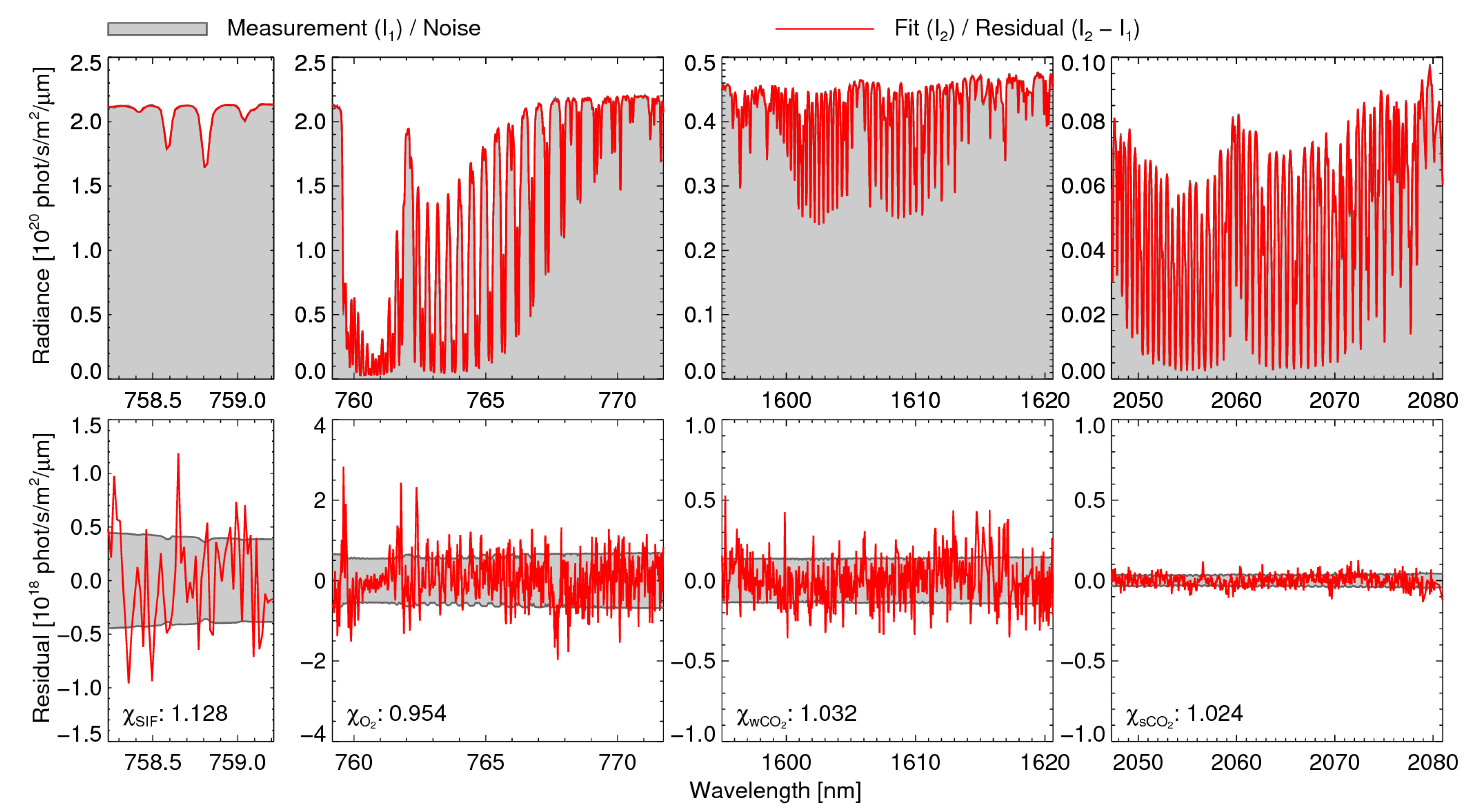
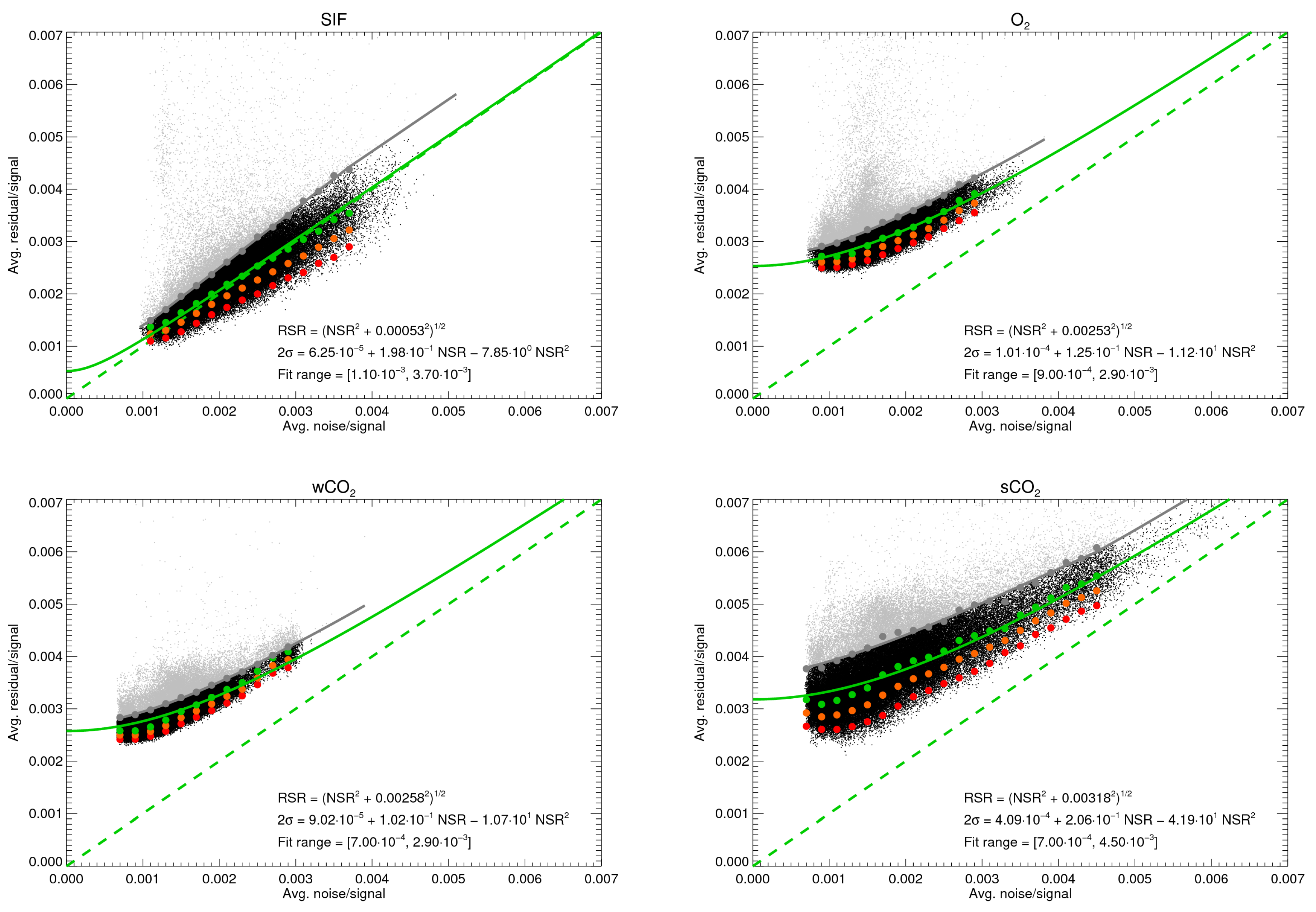
3.1. Noise Model
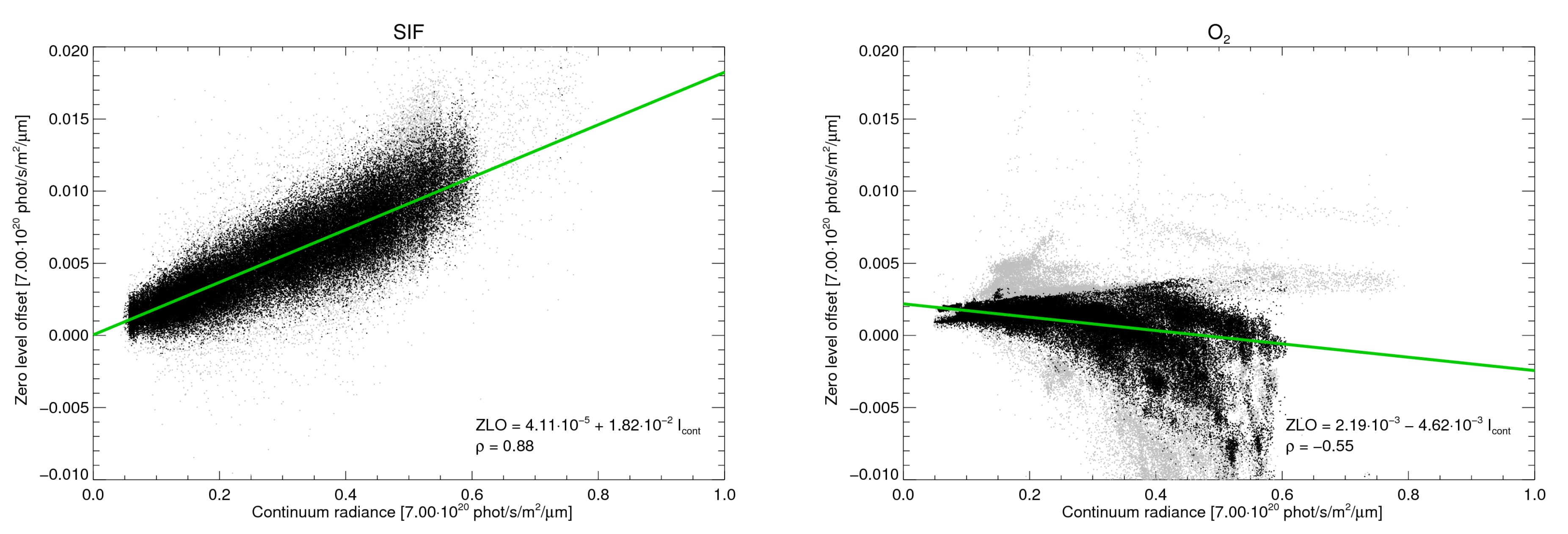
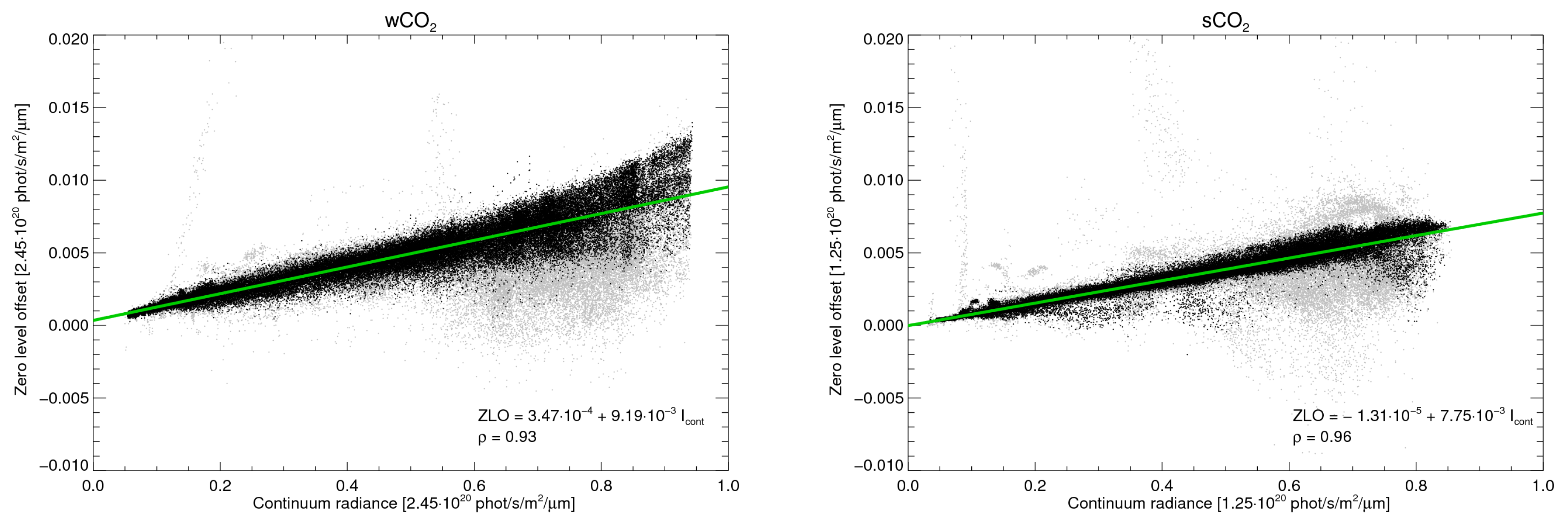
3.2. Zero Level Offset Correction
4. Postprocessing
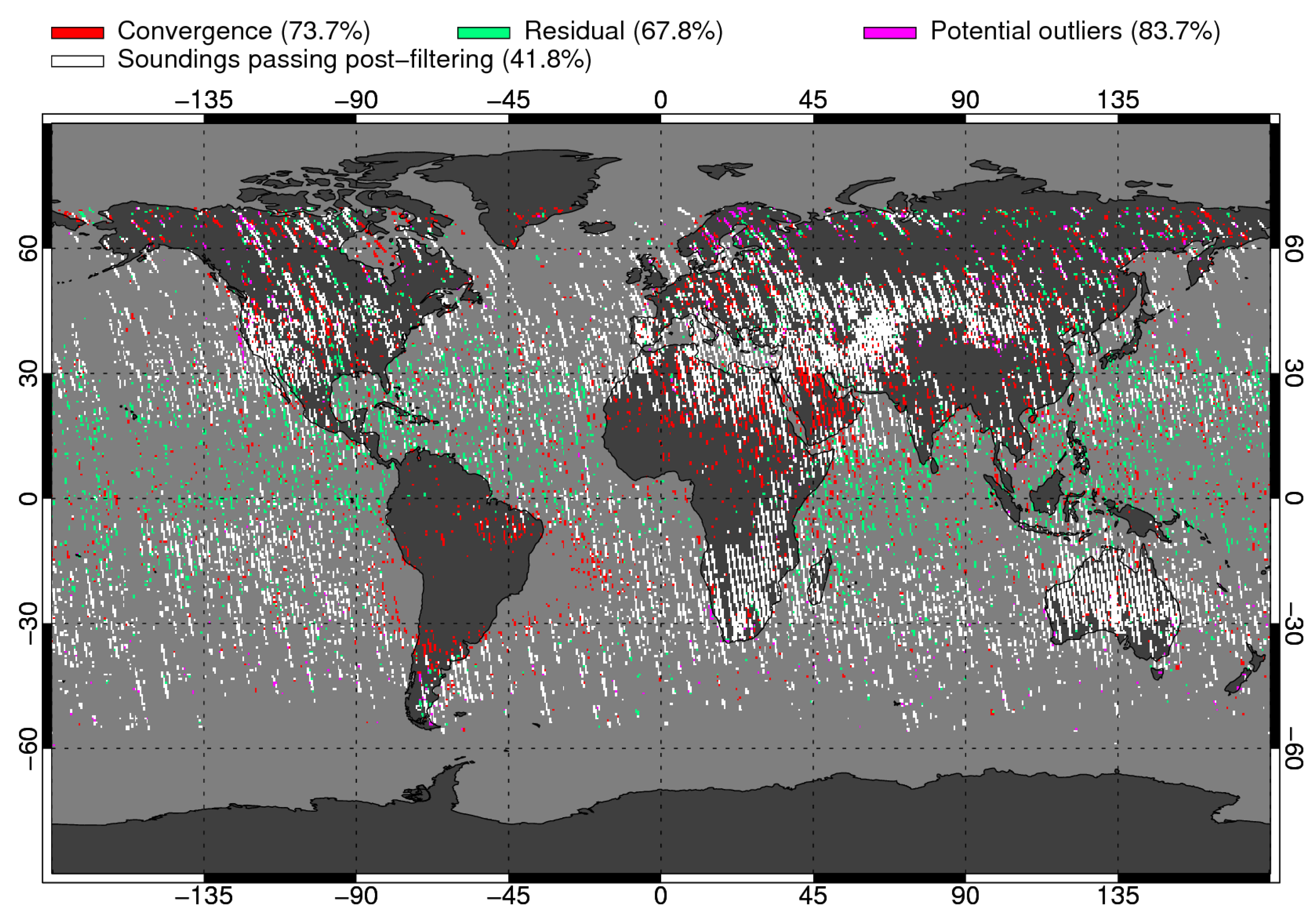
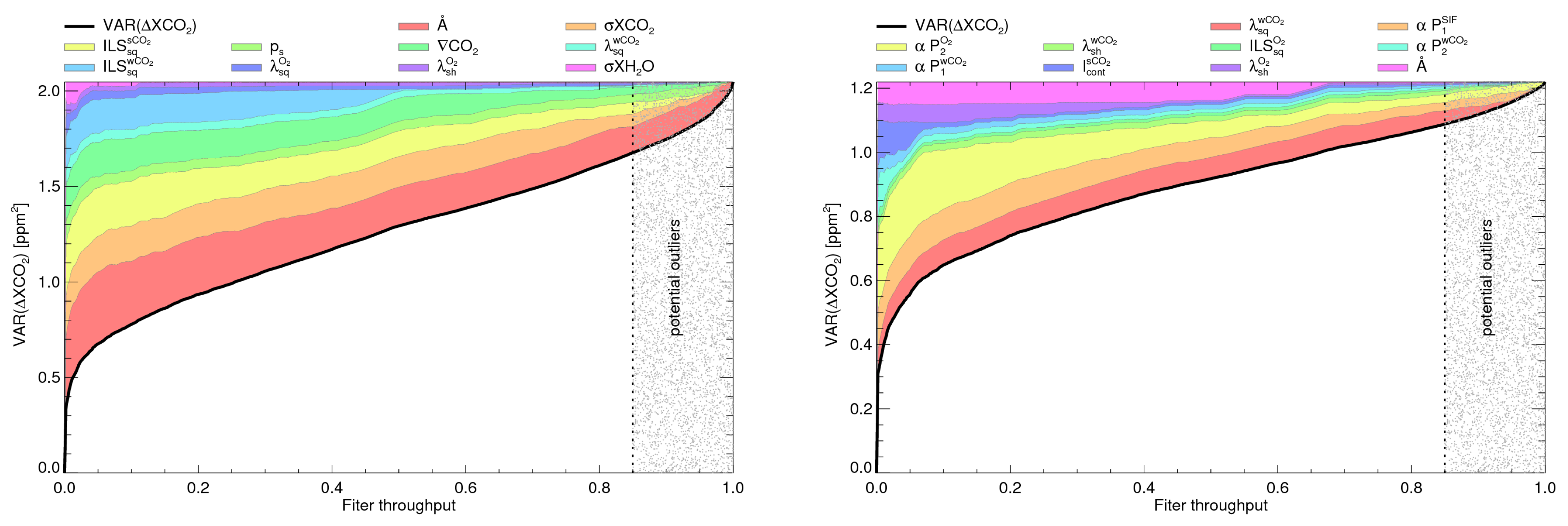
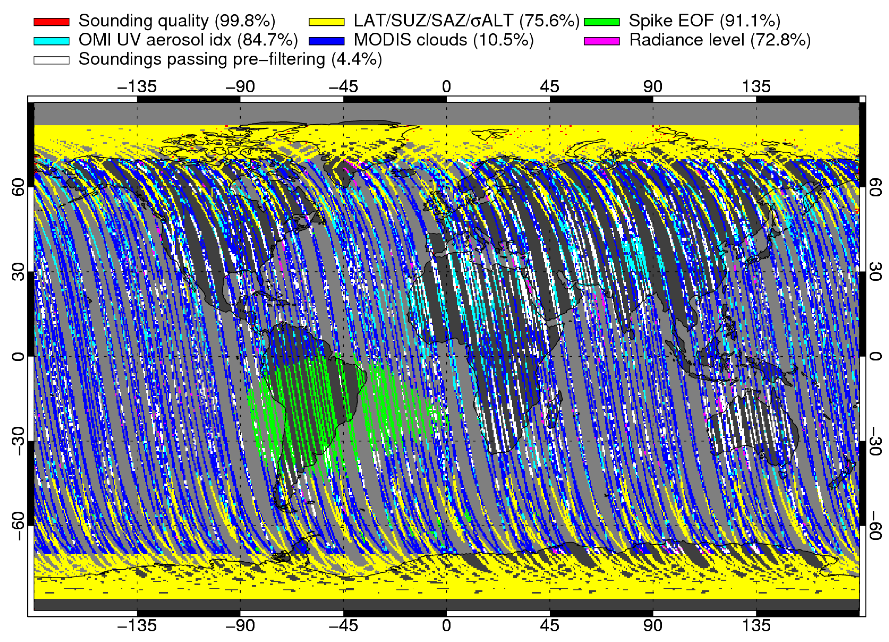
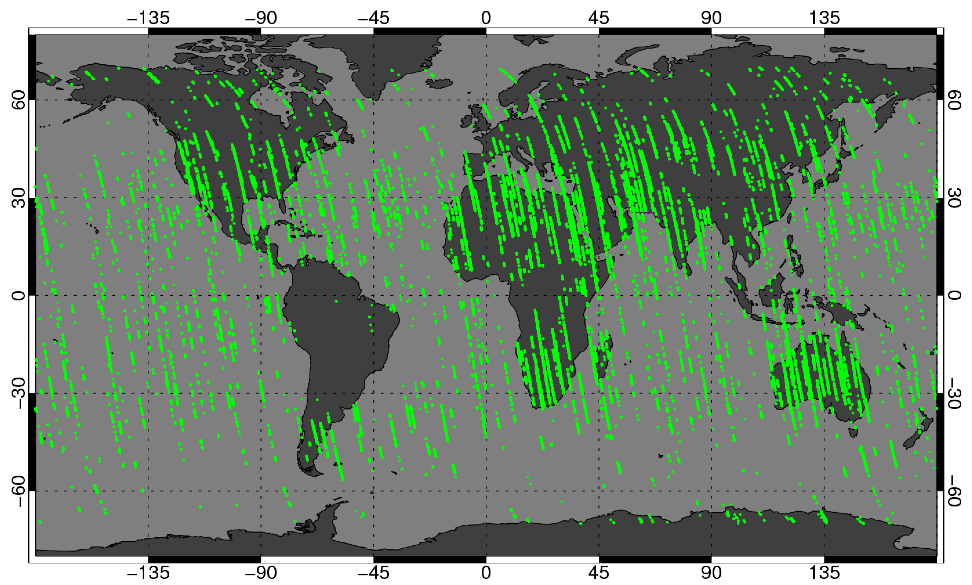
4.1. Filtering
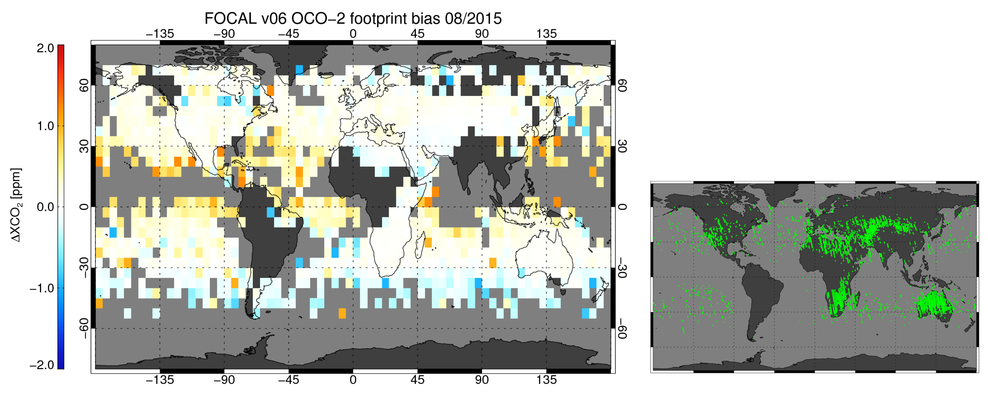
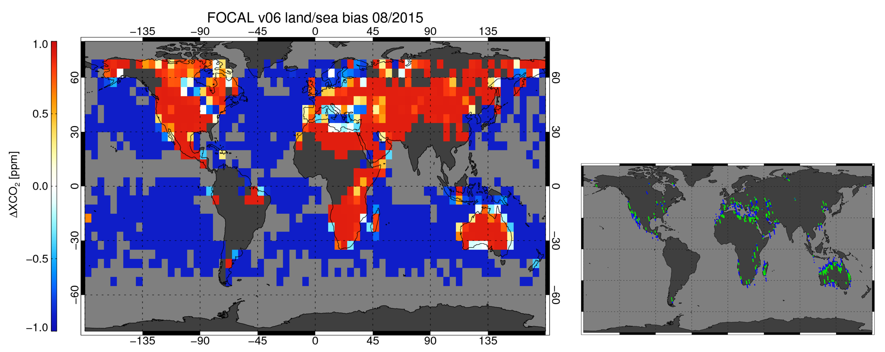
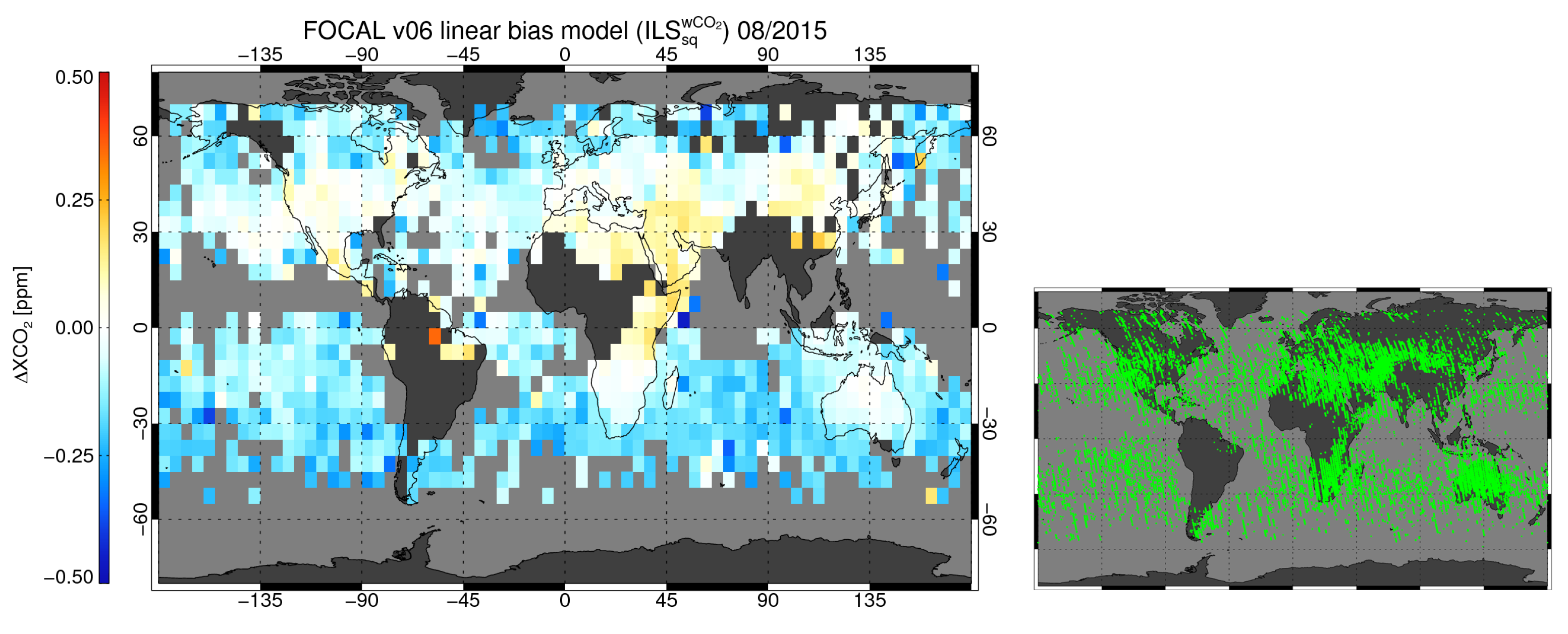
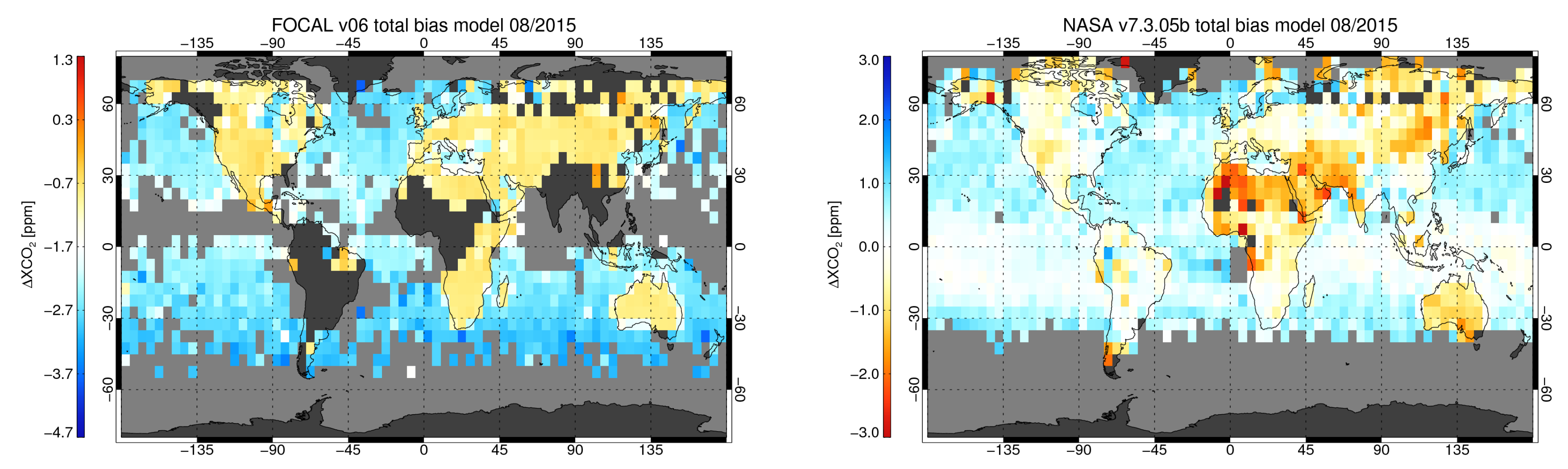
4.2. Bias Correction
5. Comparison and Validation
5.1. Model Comparison
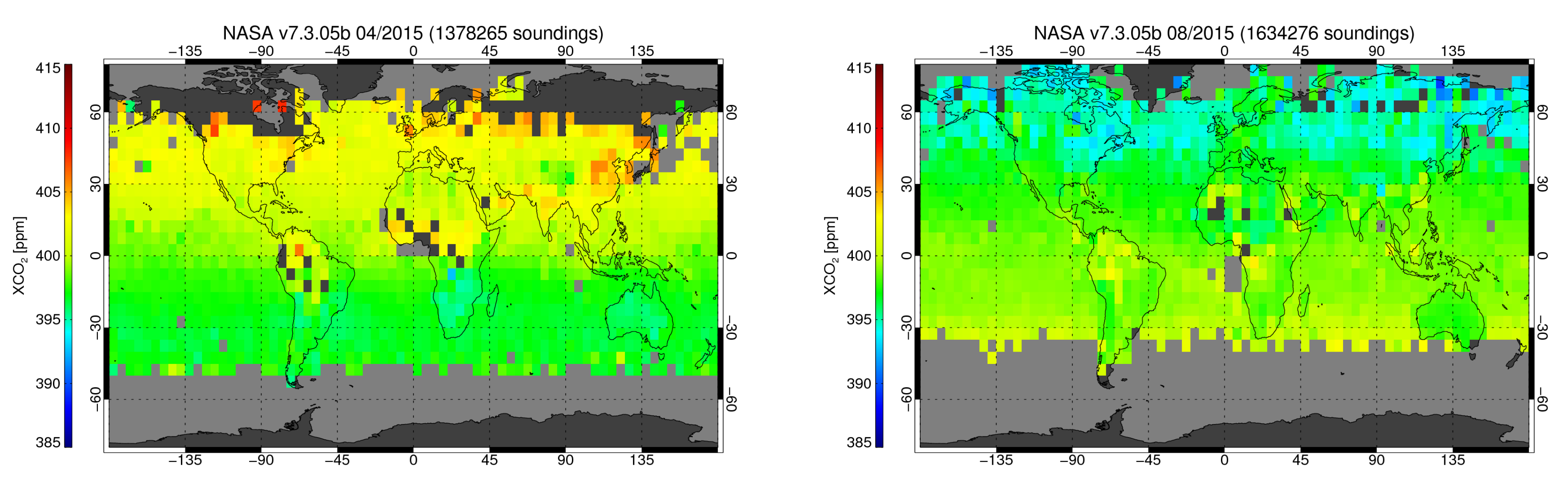
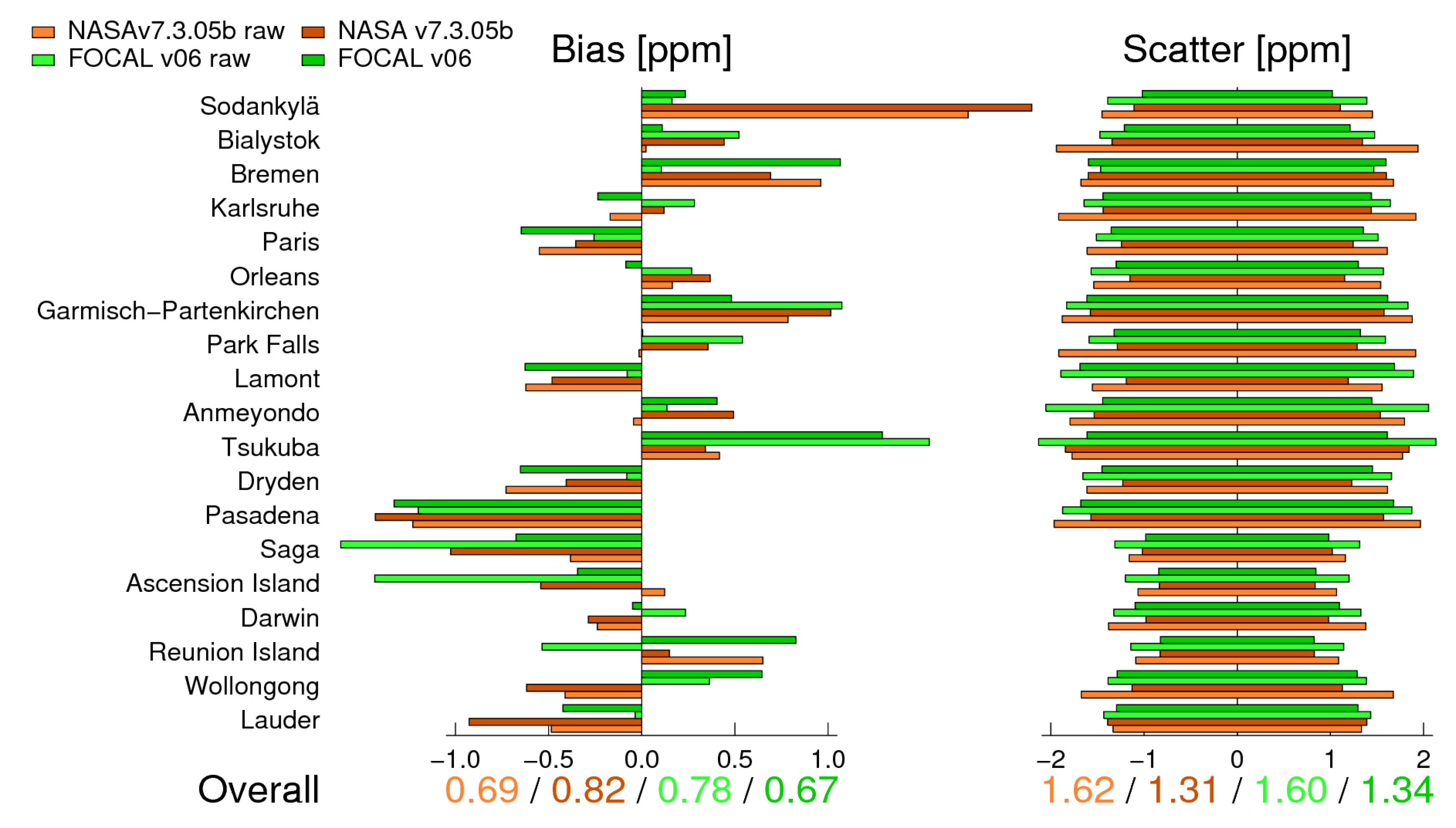
5.2. Comparison with NASA’s Operational OCO-2 L2 Product
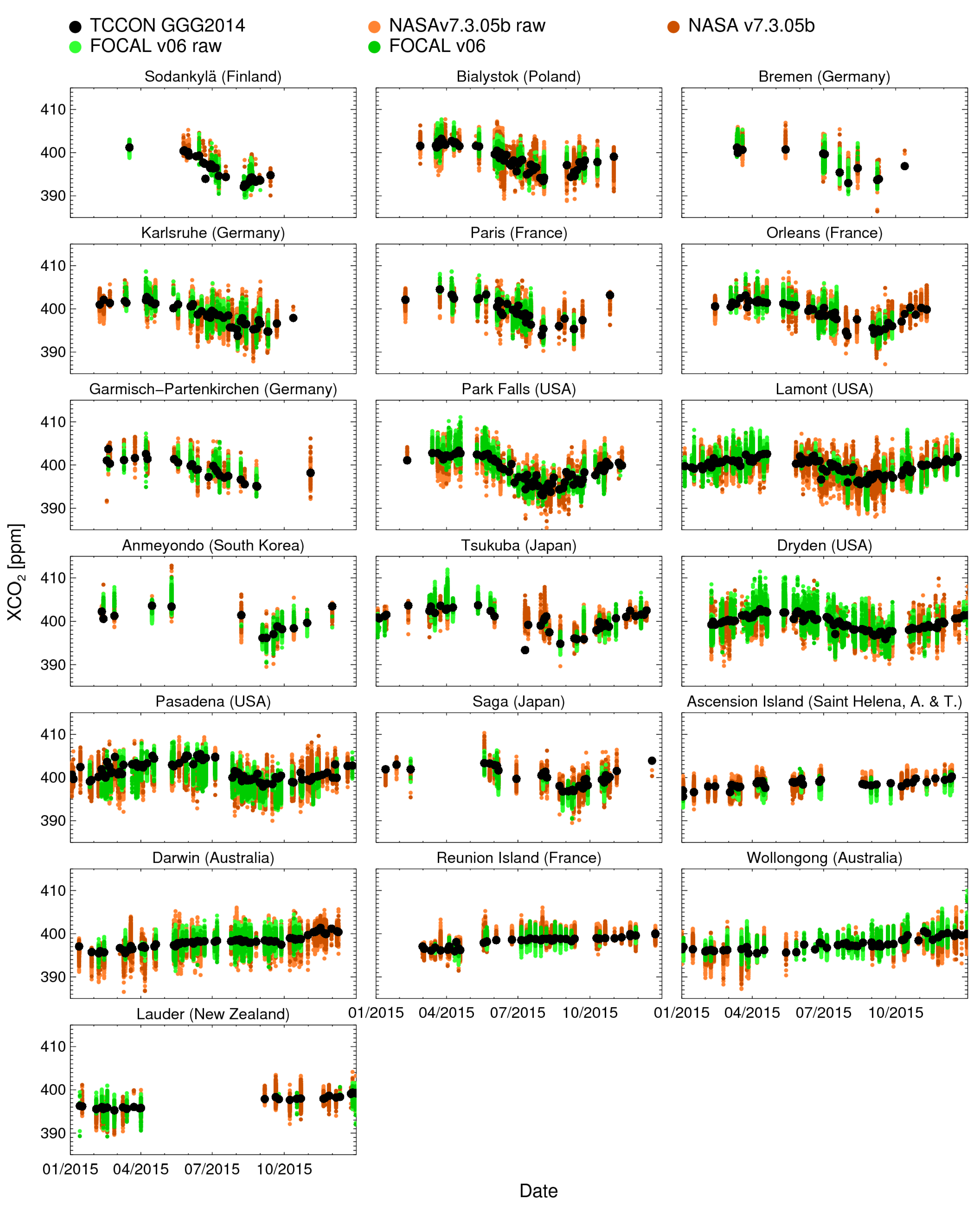
5.3. Validation with TCCON
6. Conclusions
Acknowledgments
Author Contributions
Conflicts of Interest
References
- Reuter, M.; Buchwitz, M.; Hilker, M.; Heymann, J.; Bovensmann, H.; Burrows, J.P.; Houweling, S.; Liu, Y.Y.; Nassar, R.; Chevallier, F.; et al. How much CO2 is taken up by the European Terrestrial Biosphere? Bull. Am. Meteorol. Soc. 2017, 98, 665–671. [Google Scholar] [CrossRef]
- Miller, C.E.; Crisp, D.; DeCola, P.L.; Olsen, S.C.; Randerson, J.T.; Michalak, A.M.; Alkhaled, A.; Rayner, P.; Jacob, D.J.; Suntharalingam, P.; et al. Precision requirements for space-based XCO2 data. J. Geophys. Res. 2007, 112. [Google Scholar] [CrossRef]
- Chevallier, F.; Bréon, F.M.; Rayner, P.J. Contribution of the Orbiting Carbon Observatory to the estimation of CO2 sources and sinks: Theoretical study in a variational data assimilation framework. J. Geophys. Res. 2007, 112. [Google Scholar] [CrossRef]
- Bovensmann, H.; Buchwitz, M.; Burrows, J.P.; Reuter, M.; Krings, T.; Gerilowski, K.; Schneising, O.; Heymann, J.; Tretner, A.; Erzinger, J. A remote sensing technique for global monitoring of power plant CO2 emissions from space and related applications. Atmos. Meas. Tech. 2010, 3, 781–811. [Google Scholar] [CrossRef]
- Burrows, J.P.; Hölzle, E.; Goede, A.P.H.; Visser, H.; Fricke, W. SCIAMACHY—Scanning imaging absorption spectrometer for atmospheric chartography. Acta Astronaut. 1995, 35, 445–451. [Google Scholar] [CrossRef]
- Bovensmann, H.; Burrows, J.P.; Buchwitz, M.; Frerick, J.; Noël, S.; Rozanov, V.V.; Chance, K.V.; Goede, A. SCIAMACHY—Mission objectives and measurement modes. J. Atmos. Sci. 1999, 56, 127–150. [Google Scholar] [CrossRef]
- Kuze, A.; Suto, H.; Nakajima, M.; Hamazaki, T. Thermal and near infrared sensor for carbon observation Fourier-transform spectrometer on the Greenhouse Gases Observing Satellite for greenhouse gases monitoring. Appl. Opt. 2009, 48, 6716. [Google Scholar] [CrossRef] [PubMed]
- Crisp, D.; Atlas, R.M.; Bréon, F.M.; Brown, L.R.; Burrows, J.P.; Ciais, P.; Connor, B.J.; Doney, S.C.; Fung, I.Y.; Jacob, D.J.; et al. The Orbiting Carbon Observatory (OCO) mission. Adv. Space Res. 2004, 34, 700–709. [Google Scholar] [CrossRef]
- Crisp, D.; Pollock, H.R.; Rosenberg, R.; Chapsky, L.; Lee, R.A.M.; Oyafuso, F.A.; Frankenberg, C.; O’Dell, C.W.; Bruegge, C.J.; Doran, G.B.; et al. The on-orbit performance of the Orbiting Carbon Observatory-2 (OCO-2) instrument and its radiometrically calibrated products. Atmos. Meas. Tech. 2017, 10, 59–81. [Google Scholar] [CrossRef]
- Buchwitz, M.; Rozanov, V.V.; Burrows, J.P. A near-infrared optimized DOAS method for the fast global retrieval of atmospheric CH4, CO, CO2, H2O, and N2O total column amounts from SCIAMACHY Envisat-1 nadir radiances. J. Geophys. Res. 2000, 105, 15231–15245. [Google Scholar] [CrossRef]
- Reuter, M.; Buchwitz, M.; Schneising, O.; Heymann, J.; Bovensmann, H.; Burrows, J.P. A method for improved SCIAMACHY CO2 retrieval in the presence of optically thin clouds. Atmos. Meas. Tech. 2010, 3, 209–232. [Google Scholar] [CrossRef]
- Schneising, O.; Buchwitz, M.; Reuter, M.; Heymann, J.; Bovensmann, H.; Burrows, J.P. Long-term analysis of carbon dioxide and methane column-averaged mole fractions retrieved from SCIAMACHY. Atmos. Chem. Phys. 2011, 11, 2863–2880. [Google Scholar] [CrossRef] [Green Version]
- Heymann, J.; Bovensmann, H.; Buchwitz, M.; Burrows, J.P.; Deutscher, N.M.; Notholt, J.; Rettinger, M.; Reuter, M.; Schneising, O.; Sussmann, R.; et al. SCIAMACHY WFM-DOAS XCO2: Reduction of scattering related errors. Atmos. Meas. Tech. 2012, 5, 2375–2390. [Google Scholar] [CrossRef]
- Butz, A.; Guerlet, S.; Hasekamp, O.; Schepers, D.; Galli, A.; Aben, I.; Frankenberg, C.; Hartmann, J.M.; Tran, H.; Kuze, A.; et al. Toward accurate CO2 and CH4 observations from GOSAT. Geophys. Res. Lett. 2011, 38. [Google Scholar] [CrossRef]
- Cogan, A.J.; Boesch, H.; Parker, R.J.; Feng, L.; Palmer, P.I.; Blavier, J.F.L.; Deutscher, N.M.; Macatangay, R.; Notholt, J.; Roehl, C.; et al. Atmospheric carbon dioxide retrieved from the Greenhouse gases Observing SATellite (GOSAT): Comparison with ground-based TCCON observations and GEOS-Chem model calculations. J. Geophys. Res. Atmos. 2012, 117. [Google Scholar] [CrossRef] [Green Version]
- O’Dell, C.W.; Connor, B.; Bösch, H.; O’Brien, D.; Frankenberg, C.; Castano, R.; Christi, M.; Eldering, D.; Fisher, B.; Gunson, M.; et al. The ACOS CO2 retrieval algorithm—Part 1: Description and validation against synthetic observations. Atmos. Meas. Tech. 2012, 5, 99–121. [Google Scholar] [CrossRef]
- Yoshida, Y.; Kikuchi, N.; Morino, I.; Uchino, O.; Oshchepkov, S.; Bril, A.; Saeki, T.; Schutgens, N.; Toon, G.C.; Wunch, D.; et al. Improvement of the retrieval algorithm for GOSAT SWIR XCO2 and XCH4 and their validation using TCCON data. Atmos. Meas. Tech. 2013, 6, 1533–1547. [Google Scholar] [CrossRef]
- Buchwitz, M.; Reuter, M.; Schneising, O.; Hewson, W.; Detmers, R.G.; Boesch, H.; Hasekamp, O.P.; Aben, I.; Bovensmann, H.; Burrows, J.P.; et al. Global satellite observations of column-averaged carbon dioxide and methane: The GHG-CCI XCO2 and XCH4 CRDP3 data set. Remote Sens. Environ. 2017. [Google Scholar] [CrossRef]
- Reuter, M.; Bösch, H.; Bovensmann, H.; Bril, A.; Buchwitz, M.; Butz, A.; Burrows, J.P.; O’Dell, C.W.; Guerlet, S.; Hasekamp, O.; et al. A joint effort to deliver satellite retrieved atmospheric CO2 concentrations for surface flux inversions: The ensemble median algorithm EMMA. Atmos. Chem. Phys. 2013, 13, 1771–1780. [Google Scholar] [CrossRef]
- Reuter, M.; Buchwitz, M.; Hilker, M.; Heymann, J.; Schneising, O.; Pillai, D.; Bovensmann, H.; Burrows, J.P.; Bösch, H.; Parker, R.; et al. Satellite-inferred European carbon sink larger than expected. Atmos. Chem. Phys. 2014, 14, 13739–13753. [Google Scholar] [CrossRef]
- Boesch, H.; Brown, L.; Castano, R.; Christi, M.; Connor, B.; Crisp, D.; Eldering, A.; Fisher, B.; Frankenberg, C.; Gunson, M.; et al. Orbiting Carbon Observatory-2 (OCO-2) Level 2 Full Physics Retrieval Algorithm Theoretical Basis; Version 2.0 Rev 2; National Aeronautics and Space Administration, Jet Propulsion Laboratory, California Institute of Technology: Pasadena, CA, USA, 2015.
- Eldering, A.; O’Dell, C.W.; Wennberg, P.O.; Crisp, D.; Gunson, M.R.; Viatte, C.; Avis, C.; Braverman, A.; Castano, R.; Chang, A.; et al. The Orbiting Carbon Observatory-2: First 18 months of science data products. Atmos. Meas. Tech. 2017, 10, 549. [Google Scholar] [CrossRef]
- Reuter, M.; Buchwitz, M.; Schneising, O.; Noël, S.; Rozanov, V.; Bovensmann, H.; Burrows, J.P. A fast atmospheric trace gas retrieval for hyperspectral instruments approximating multiple scattering—Part 1: Radiative transfer and a potential OCO-2 XCO2 retrieval setup. Remote Sens. 2017. submitted. [Google Scholar]
- Eldering, A.; Pollock, R.; Lee, R.; Rosenberg, R.; Oyafuso, F.; Crisp, D.; Chapsky, L.; Granat, R. Orbiting Carbon Observatory-2 (OCO-2) - LEVEL 1B - Algorithm Theoretical Basis; Version 1.2 Rev 1; National Aeronautics and Space Administration, Jet Propulsion Laboratory, California Institute of Technology: Pasadena, CA, USA, 2015.
- Stammes, P. OMI Algorithm Theoretical Basis Document, Volume III, Clouds, Aerosols, and Surface UV Irradiance (ATBD-OMI-03); Royal Netherlands Meteorological Institute (KNMI): De Bilt, The Netherlands, 2002. [Google Scholar]
- Ackerman, S.; Frey, R.; Strabala, K.; Liu, Y.; Gumley, L.; Baum, B.; Menzel, P. Discriminating Clear-Sky from Cloud with MODIS—Algorithm Theoretical Basis Document (MOD35); Version 6.1; Cooperative Institute for Meteorological Satellite Studies, University of Wisconsin—Madison: Madison, WI, USA, 2010. [Google Scholar]
- Heymann, J.; Reuter, M.; Hilker, M.; Buchwitz, M.; Schneising, O.; Bovensmann, H.; Burrows, J.P.; Kuze, A.; Suto, H.; Deutscher, N.M.; et al. Consistent satellite XCO2 retrievals from SCIAMACHY and GOSAT using the BESD algorithm. Atmos. Meas. Tech. 2015, 8, 2961–2980. [Google Scholar] [CrossRef]
- Hu, C.; Lee, Z.; Franz, B. Chlorophyll-a algorithms for oligotrophic oceans: A novel approach based on three-band reflectance difference. J. Geophys. Res. Oceans 2012, 117. [Google Scholar] [CrossRef]
- Chevallier, F.; Ciais, P.; Conway, T.J.; Aalto, T.; Anderson, B.E.; Bousquet, P.; Brunke, E.G.; Ciattaglia, L.; Esaki, Y.; Fröhlich, M.; et al. CO2 surface fluxes at grid point scale estimated from a global 21 year reanalysis of atmospheric measurements. J. Geophys. Res. 2010, 115. [Google Scholar] [CrossRef]
- Chevallier, F. Validation report for the inverted CO2 fluxes, v16r1. CAMS deliverable CAMS73_2015S2_ D73.1.4.2-1979-2016-v1_201707. 2017. Available online: https://atmosphere.copernicus.eu/sites/default/files/FileRepository/Resources/Validation-reports/Fluxes/CAMS73_2015SC2_D73.1.4.2-1979-2016-v1_201707_final.pdf (accessed on 29 October 2017).
- Rodgers, C.D. Inverse Methods for Atmospheric Sounding: Theory and Practice; World Scientific Publishing: Singapore, 2000. [Google Scholar]
- Wunch, D.; Toon, G.C.; Blavier, J.F.L.; Washenfelder, R.A.; Notholt, J.; Connor, B.J.; Griffith, D.W.T.; Sherlock, V.; Wennberg, P.O. The Total Carbon Column Observing Network (TCCON). Philos. Trans. R. Soc. Lond. Ser. A Math. Phys. Eng. Sci. 2011, 369, 2087–2112. [Google Scholar] [CrossRef] [PubMed]
- Reuter, M.; Bovensmann, H.; Buchwitz, M.; Burrows, J.P.; Connor, B.J.; Deutscher, N.M.; Griffith, D.W.T.; Heymann, J.; Keppel-Aleks, G.; Messerschmidt, J.; et al. Retrieval of atmospheric CO2 with enhanced accuracy and precision from SCIAMACHY: Validation with FTS measurements and comparison with model results. J. Geophys. Res. 2011, 116. [Google Scholar] [CrossRef]
- Kivi, R.; Heikkinen, P.; Kyro, E. TCCON data from Sodankyla, Finland, Release GGG2014R0. In TCCON Data Archive; Carbon Dioxide Information Analysis Center (CDIAC): Sacramento, CA, USA, 2014. [Google Scholar]
- Deutscher, N.; Notholt, J.; Messerschmidt, J.; Weinzierl, C.; Warneke, T.; Petri, C.; Grupe, P.; Katrynski, K. TCCON data from Bialystok, Poland, Release GGG2014R1. In TCCON Data Archive; Carbon Dioxide Information Analysis Center (CDIAC): Sacramento, CA, USA, 2014. [Google Scholar]
- Notholt, J.; Petri, C.; Warneke, T.; Deutscher, N.; Buschmann, M.; Weinzierl, C.; Macatangay, R.; Grupe, P. TCCON data from Bremen, Germany, Release GGG2014R0. In TCCON Data Archive; Carbon Dioxide Information Analysis Center (CDIAC): Sacramento, CA, USA, 2014. [Google Scholar]
- Hase, F.; Blumenstock, T.; Dohe, S.; Groß, J.; Kiel, M. TCCON data from Karlsruhe, Germany, Release GGG2014R1. In TCCON Data Archive; Carbon Dioxide Information Analysis Center (CDIAC): Sacramento, CA, USA, 2014. [Google Scholar]
- Te, Y.; Jeseck, P.; Janssen, C. TCCON data from Paris, France, Release GGG2014R0. In TCCON Data Archive; Carbon Dioxide Information Analysis Center (CDIAC): Sacramento, CA, USA, 2014. [Google Scholar]
- Warneke, T.; Messerschmidt, J.; Notholt, J.; Weinzierl, C.; Deutscher, N.; Petri, C.; Grupe, P.; Vuillemin, C.; Truong, F.; Schmidt, M.; et al. TCCON data from Orleans, France, Release GGG2014R0. In TCCON Data Archive; Carbon Dioxide Information Analysis Center (CDIAC): Sacramento, CA, USA, 2014. [Google Scholar]
- Sussmann, R.; Rettinger, M. TCCON data from Garmisch, Germany, Release GGG2014R0. In TCCON Data Archive; Carbon Dioxide Information Analysis Center (CDIAC): Sacramento, CA, USA, 2014. [Google Scholar]
- Wennberg, P.O.; Roehl, C.; Wunch, D.; Toon, G.C.; Blavier, J.F.; Washenfelder, R.; Keppel-Aleks, G.; Allen, N.; Ayers, J. TCCON data from Park Falls, Wisconsin, USA, Release GGG2014R0. In TCCON Data Archive; Carbon Dioxide Information Analysis Center (CDIAC): Sacramento, CA, USA, 2014. [Google Scholar]
- Wennberg, P.O.; Wunch, D.; Roehl, C.; Blavier, J.F.; Toon, G.C.; Allen, N.; Dowell, P.; Teske, K.; Martin, C.; Martin, J. TCCON data from Lamont, Oklahoma, USA, Release GGG2014R1. In TCCON Data Archive; Carbon Dioxide Information Analysis Center (CDIAC): Sacramento, CA, USA, 2014. [Google Scholar]
- Goo, T.Y.; Oh, Y.S.; Velazco, V.A. TCCON data from Anmeyondo, South Korea, Release GGG2014R0. In TCCON Data Archive; Carbon Dioxide Information Analysis Center (CDIAC): Sacramento, CA, USA, 2014. [Google Scholar]
- Morino, I.; Matsuzaki, T.; Shishime, A. TCCON data from Tsukuba, Ibaraki, Japan, 125HR, Release GGG2014R1. In TCCON Data Archive; Carbon Dioxide Information Analysis Center (CDIAC): Sacramento, CA, USA, 2014. [Google Scholar]
- Iraci, L.; Podolske, J.; Hillyard, P.; Roehl, C.; Wennberg, P.O.; Blavier, J.F.; Landeros, J.; Allen, N.; Wunch, D.; Zavaleta, J.; et al. TCCON data from Armstrong Flight Research Center, Edwards, CA, USA, Release GGG2014R1. In TCCON Data Archive; Carbon Dioxide Information Analysis Center (CDIAC): Sacramento, CA, USA, 2014. [Google Scholar]
- Wennberg, P.O.; Wunch, D.; Yavin, Y.; Toon, G.C.; Blavier, J.F.; Allen, N.; Keppel-Aleks, G. TCCON data from Jet Propulsion Laboratory, Pasadena, California, USA, Release GGG2014R0. In TCCON Data Archive; Carbon Dioxide Information Analysis Center (CDIAC): Sacramento, CA, USA, 2014. [Google Scholar]
- Shiomi, K.; Kawakami, S.; Ohyama, H.; Arai, K.; Okumura, H.; Taura, C.; Fukamachi, T.; Sakashita, M. TCCON data from Saga, Japan, Release GGG2014R0. In TCCON Data Archive; Carbon Dioxide Information Analysis Center (CDIAC): Sacramento, CA, USA, 2014. [Google Scholar]
- Feist, D.G.; Arnold, S.G.; John, N.; Geibel, M.C. TCCON data from Ascension Island, Saint Helena, Ascension and Tristan da Cunha, Release GGG2014R0. In TCCON Data Archive; Carbon Dioxide Information Analysis Center (CDIAC): Sacramento, CA, USA, 2014. [Google Scholar]
- Griffith, D.W.T.; Deutscher, N.; Velazco, V.A.; Wennberg, P.O.; Yavin, Y.; Aleks, G.K.; Washenfelder, R.; Toon, G.C.; Blavier, J.F.; Murphy, C.; et al. TCCON data from Darwin, Australia, Release GGG2014R0. In TCCON Data Archive; Carbon Dioxide Information Analysis Center (CDIAC): Sacramento, CA, USA, 2014. [Google Scholar]
- De Maziere, M.; Sha, M.K.; Desmet, F.; Hermans, C.; Scolas, F.; Kumps, N.; Metzger, J.M.; Duflot, V.; Cammas, J.P. TCCON data from Reunion Island (La Reunion), France, Release GGG2014R0. In TCCON Data Archive; Carbon Dioxide Information Analysis Center (CDIAC): Sacramento, CA, USA, 2014. [Google Scholar]
- Griffith, D.W.T.; Velazco, V.A.; Deutscher, N.; Murphy, C.; Jones, N.; Wilson, S.; Macatangay, R.; Kettlewell, G.; Buchholz, R.R.; Riggenbach, M. TCCON data from Wollongong, Australia, Release GGG2014R0. In TCCON Data Archive; Carbon Dioxide Information Analysis Center (CDIAC): Sacramento, CA, USA, 2014. [Google Scholar]
- Sherlock, V.; Connor, B.; Robinson, J.; Shiona, H.; Smale, D.; Pollard, D. TCCON data from Lauder, New Zealand, 125HR, Release GGG2014R0. In TCCON Data Archive; Carbon Dioxide Information Analysis Center (CDIAC): Sacramento, CA, USA, 2014. [Google Scholar]
- Taylor, T.E.; O’Dell, C.W.; Partain, P.T.; Cronk, H.Q.; Nelson, R.R.; Rosenthal, E.J.; Chang, A.Y.; Osterman, G.B.; Pollock, R.H.; Gunson, M.R. Orbiting Carbon Observatory-2 (OCO-2) cloud screening algorithms: Validation against collocated MODIS and CALIOP data. Atmos. Meas. Tech. 2016, 9, 973. [Google Scholar] [CrossRef]
- Buchwitz, M.; Reuter, M.; Bovensmann, H.; Pillai, D.; Heymann, J.; Schneising, O.; Rozanov, V.; Krings, T.; Burrows, J.P.; Boesch, H.; et al. Carbon Monitoring Satellite (CarbonSat): Assessment of atmospheric CO2 and CH4 retrieval errors by error parameterization. Atmos. Meas. Tech. 2013, 6, 3477–3500. [Google Scholar] [CrossRef]


| Parameter | Lower Threshold | Upper Threshold | Variance Reduction [%] | |
|---|---|---|---|---|
| Land | Å | 1.6669 | - | 38 |
| XCO [ppm] | - | 1.2963 | 17 | |
| - | 1.0022 | 16 | ||
| p [p] | −1.6435 × 10 | 2.2603 × 10 | 11 | |
| ∇CO [ppm] | 5.2509 | 5.9995 | 11 | |
| [nm] | −5.2186 × 10 | 3.9367 × 10 | 2 | |
| - | 1.0041 | 1 | ||
| [nm] | - | −2.5907 × 10 | 2 | |
| [nm] | −6.6146 × 10 | 9.2043 × 10 | 1 | |
| XHO [ppm] | - | 15.705 | 1 | |
| Sea | [nm] | −3.1372 × 10 | −8.2869 × 10 | 32 |
| −2.3184 × 10 | 3.4846 × 10 | 20 | ||
| - | 1.7900 × 10 | 19 | ||
| [nm] | - | 2.1023 × 10 | 9 | |
| - | 1.0175 | 4 | ||
| - | −2.1247 × 10 | 5 | ||
| 3.2736 × 10 | - | 4 | ||
| [1.25 × 10 Ph/s/m/m] | 5.6468 × 10 | - | 4 | |
| [nm] | −3.4860 × 10 | - | 2 | |
| Å | 1.9014 | - | 2 |
© 2017 by the authors. Licensee MDPI, Basel, Switzerland. This article is an open access article distributed under the terms and conditions of the Creative Commons Attribution (CC BY) license (http://creativecommons.org/licenses/by/4.0/).
Share and Cite
Reuter, M.; Buchwitz, M.; Schneising, O.; Noël, S.; Bovensmann, H.; Burrows, J.P. A Fast Atmospheric Trace Gas Retrieval for Hyperspectral Instruments Approximating Multiple Scattering—Part 2: Application to XCO2 Retrievals from OCO-2. Remote Sens. 2017, 9, 1102. https://doi.org/10.3390/rs9111102
Reuter M, Buchwitz M, Schneising O, Noël S, Bovensmann H, Burrows JP. A Fast Atmospheric Trace Gas Retrieval for Hyperspectral Instruments Approximating Multiple Scattering—Part 2: Application to XCO2 Retrievals from OCO-2. Remote Sensing. 2017; 9(11):1102. https://doi.org/10.3390/rs9111102
Chicago/Turabian StyleReuter, Maximilian, Michael Buchwitz, Oliver Schneising, Stefan Noël, Heinrich Bovensmann, and John P. Burrows. 2017. "A Fast Atmospheric Trace Gas Retrieval for Hyperspectral Instruments Approximating Multiple Scattering—Part 2: Application to XCO2 Retrievals from OCO-2" Remote Sensing 9, no. 11: 1102. https://doi.org/10.3390/rs9111102