Improving the Triple-Carrier Ambiguity Resolution with a New Ionosphere-Free and Variance-Restricted Method

1
College of Automation, Harbin Engineering University, Harbin 150001, China
2
Academy of Opto-Electronics, Chinese Academy of Sciences, Beijing 100094, China
*
Author to whom correspondence should be addressed.
Remote Sens. 2017, 9(11), 1108; https://doi.org/10.3390/rs9111108
Submission received: 22 September 2017
/
Revised: 24 October 2017
/
Accepted: 25 October 2017
/
Published: 30 October 2017
(This article belongs to the Special Issue Multi-Constellation Global Navigation Satellite Systems: Methods and Applications)
Abstract
:The ionospheric bias and the combined observation noise are two crucial factors affecting the reliability of the triple-carrier ambiguity resolution (TCAR). In order to obtain a better reliability of TCAR, a new ionosphere-free and variance-restricted TCAR method is proposed through exploring the ambiguity link between each step of TCAR. The method constructs an ionosphere-free combination and simultaneously restricts the combined observation noise with respect to the wavelength to a sufficiently low level for each step of TCAR. The performance of the proposed method is tested by the datasets from the BeiDou navigation satellite system (BDS), with the baseline varying from 7.7 km to 68.8 km. Comparing with the state-of-the-art TCAR methods, the experimental results indicate that the proposed method can obtain a better performance of ambiguity resolution, even though the double-differenced ionospheric delay increases up to 72.4 cm at the baseline of 68.8 km.
1. Introduction
Integer ambiguity resolution is the key technique for high-precision relative positioning using carrier phase observation such as real-time kinematic (RTK) [1]. With the modernization of global navigation satellite system (GNSS), significant efforts have been made to achieve reliable ambiguity resolution by using the triple-frequency signals. The triple-carrier ambiguity resolution (TCAR) method proposed by the authors of [2,3] is one of the widely-used approaches for resolving the triple-frequency ambiguity in a short baseline case so that the ionospheric error can be neglected. When the ionospheric bias cannot be neglected, especially in medium and long baseline cases, much research has also been done to improve its performance [4,5,6,7]. A common conclusion is that both the ionospheric bias and combined observation noise are two crucial factors for the reliability of TCAR [4,8]. Therefore, it is very necessary to eliminate the ionospheric bias and restrict the combined observation noise level simultaneously to improve the reliability of TCAR.
Considering these two crucial factors for TCAR, the ionosphere-estimated method can be used to compensate the effect of ionospheric bias without amplifying the observation noise [6,9]. However, the performance of the ionosphere-estimated method depends on the precision of the ionospheric model, which includes a functional and stochastic model. Moreover, the increased ionosphere-related parameters will reduce the strength of the estimated-model [10]. The rate of total electrical content (TEC) corrections can be utilized to improve the strength of the ionosphere-estimated model, and it has proven to be efficient for different latitudes and ionospheric conditions [11,12]. In addition to the ionosphere-estimated method, most studies of TCAR focus on choosing the optimal combination coefficients among triple-frequency observations. These studies aim at suppressing the effect of ionospheric bias and combined observation noise [4,5,8,13,14]. The coefficients can be determined based on different categories to suppress these two kinds of observation errors. The widely-used category includes the ionosphere-free combination [13,15,16,17] and the ionosphere-reduced combination [4]. The ionosphere-free combination ensures the absence of ionospheric bias, but the combined observation noise is largely amplified, which will worsen ambiguity resolution performance [18,19]. Therefore, a moving average method has to be used to restrict the effect of combined observation noise [7,13,17,20,21]. Furthermore, the ionosphere-reduced combination can also be applied because it is in essence a trade-off between the ionospheric effect reduction and observation variance restriction. It aims at suppressing the effect of ionospheric bias and combined observation noise simultaneously [4]. Nevertheless, the residual of ionospheric delay is still a threat for the reliability of TCAR.
The ionosphere is difficult to be predicted or modeled precisely because it is subjected to undetermined variation in temporal and spatial dimensions [22]. Therefore, the reliability of the ionosphere-estimated method has its limitations. In contrast, the observation combination method has enormous potential in mitigating the effect of ionospheric bias so that the reliability of TCAR can be improved [5,8,13]. Typically, the ionosphere-free combination is usually used for eliminating the effect of ionospheric bias on TCAR. However, the current ionosphere-free combined methods still suffer from the contradiction between eliminating ionospheric bias and suppressing combined observation noise. The contradiction is reflected by the fact that, if the ionospheric bias is eliminated, the combined observation noise will be amplified. If the combined observation noise is restricted, the ionospheric bias is difficult to be eliminated for the traditional TCAR methods. Although the traditional ionosphere-free combination method takes the advantage of ambiguity-corrected observations from previous steps to restrict the combined observation noise with respect to the wavelength, the corresponding combination still does not successfully restrict the noise with respect to the wavelength to a sufficiently low level [13,17]. To restrict the combined observation noise level under the ionosphere-free combination, we propose an ionosphere-free and variance-restricted (IFVR) TCAR method in this contribution. “Variance-restricted” means the combined observation noise with respect to the wavelength can be restricted to a sufficiently low level so as to achieve reliable ambiguity resolution. The method takes into account the available information of the ambiguity link between different steps, which can be used to build a relationship between observations with respect to different frequencies. This relationship can provide an opportunity to form an optimal combination method so that the ionospheric bias can be eliminated and the combined observation noise can be restricted simultaneously. Taking advantages of ambiguity links between each step of TCAR for the proposed method, a better ambiguity resolution performance can therefore be anticipated.
2. Methodology
In order to demonstrate the proposed TCAR method, we will briefly review the general linear combinations between the double-differenced code and carrier phase observations, shown by [4].
where combination coefficients (i, j, k) ∈ Z are the arbitrary integer and ft (t = 1, 2, 3) denote BDS three frequency signals, i.e., f1 = 1561.098 MHz, f2 = 1207.140 MHz and f3 = 1268.520 MHz, respectively; p and φ represent code and phase observations in meters, respectively; ρ describes the non-dispersive terms including geometric distance and the tropospheric delay in meters; I1 is the first-order ionospheric delay on frequency f1 in meters; λ(i,j,k) and N(i,j,k) are wavelength in meters and ambiguity in cycles for different coefficients combination; εp and εφ represent noise of double-differenced code and phase observations, respectively. The ionospheric scale factor β(i,j,k), the noise scale factor γ(i,j,k), wavelength λ(i,j,k), and ambiguity N(i,j,k) based on the combination, are defined as (Feng 2008)
where c is the speed of light.
Similar to the traditional TCAR methods, the proposed TCAR method comprises three steps: extra-wide-lane (EWL), wide-lane (WL) and narrow-lane (NL) ambiguity resolution. EWL ambiguity can be reliably resolved by previous studies [4,6,7], but rapid and reliable WL and NL ambiguity resolution is still challenging because of both ionospheric bias and the combined observation noise [6]. Therefore, the proposed TCAR method focuses on finding a better WL and NL combination method to eliminate ionospheric bias and restrict combined observation noise simultaneously. To simplify the quantitative analysis below, we assume all un-differenced observations are independent with each other, the observations among different frequencies have the same precision, i.e., un-differenced code and phase precision take 30 cm and 3 mm, respectively. Thus, the standard deviations (STD) of corresponding double-differenced observations are σp = 60 cm and σφ = 6 mm, respectively. The proposed TCAR method can be implemented by the following three-step procedure.
2.1. EWL Ambiguity Resolution
The widely-used EWL combination can be expressed as [4,6]
where φEWL represents EWL combination: the corresponding wavelength is λEWL ≈ 4.88 m. Based on the assumed observation precision, the ratio of the noise to the wavelength is σEWL/λEWL ≈ 0.09 cycles. The sufficiently low σEWL/λEWL indicates the success rate of EWL ambiguity resolution by using the constructed EWL combination is close to 100%.
2.2. WL Ambiguity Resolution
When the EWL ambiguity is correctly resolved, EWL resolved ambiguity can be used in WL ambiguity resolution. First, two widely-used WL combinations φ(1,−1,0) and φ(1,0,−1) are constructed [20,23], and then the ambiguity link between EWL and WL ambiguities can be formed as
Using (4), φ(1,−1,0) and φ(1,0,−1) contain the same ambiguity values N(1,0,−1). The characteristic provides a new WL ionosphere-free combination method, shown by
where φWL1 denotes WL ionosphere-free combination. In order to eliminate the ionospheric bias and retain the geometry terms, the values of coefficient set ≈ −19.66 and ≈ 20.66. The corresponding wavelength and noise are λWL1 = a1λ(1,−1,0) + a2λ(1,0,−1) ≈ 4.52 m and σWL1 ≈ 114.4 σφ, respectively.
In the new WL combination, it can be found that the ratio of the noise to the wavelength σWL1/λWL1 is only 0.15 cycles, although the noise has been amplified by about 114.4 times. Therefore, the new WL combination method can sufficiently restrict the combined observation noise under ionosphere-free combination, which is able to obtain a better ambiguity resolution performance.
Because of the presence of geometry terms, the rank deficiency issue exists for (5). Therefore, additional ionosphere-free combination should be constructed. Furthermore, the combination to be constructed and φWL1 must be mutually independent. One option is to construct an ionosphere-free combination by using code observations [19]. In view of the lower precision of code observations, the STD of combined observation noise using the code observation will be enlarged to meter level, e.g., the noise of ionosphere-free combination would reach up to 1.74 m by using f1 and f2 code observations [4,19]. In order to avoid the enlarged observation noise under the ionosphere-free combination, another new WL ionosphere-free combination contained WL ambiguity N(1,0,−1) is constructed taking full advantage of EWL ambiguity-corrected observation = φ(0,−1,1) − λ(0,−1,1) , written as
where φWL2 denotes another WL ionosphere-free combination; (l,m,n) ∈ Z represents combined coefficients of code observation. In order to construct ionosphere-free combination and retain geometry terms, the coefficients set and . The corresponding wavelength and noise are λWL2 = b2λ(1,0,−1) ≈ 2.84β(l,m,n) m and , respectively.
The new φWL2 eliminates the rank deficiency issue of (5), which is independent with φWL1 because of the introduction of code observations. Meanwhile, in order to obtain the best reliability of WL ambiguity resolution, the minimization criterion of σWL2/λWL2 should be satisfied. In this paper, the integer coefficients of the code observation are selected as (l,m,n) = (0,0,1), the corresponding coefficients are b1 ≈ −4.20 and b2 ≈ 4.20, respectively. The integer coefficient selection is detailed in Appendix A. As a result, the wavelength λWL2 is 4.30 m and the ratio of the noise to the wavelength is σWL2/λWL2 ≈ 0.23 cycles based on the assumed observation precision.
These two WL ionosphere-free combinations from (5) and (6) take full advantage of ambiguity links and ambiguity-corrected observations to restrict the combined observation noise with respect to wavelength sufficiently. Moreover, because the two WL observations contain the same WL ambiguity N(1,0,−1) depending on the ambiguity link between the EWL and WL ambiguity, the strength of the WL ambiguity model can be improved by these advantages. Using these two WL ionosphere-free combinations, we construct a new linear model for WL ambiguity resolution. In view of presence of non-dispersive terms, the residual tropospheric bias also needs to be taken into account as estimated parameter to compensate the tropospheric bias, which is detailed in Section 3. Therefore, the WL linear model writes
where Φ represents the vector of modelled combined observations; H denotes the geometry matrix; m is tropospheric mapping function; b includes baseline components; τ is zenith tropospheric wet delay (ZWD); N(1,0,−1) is vector of ambiguities; I is identity matrix. After applying least-square estimation, the WL ambiguities N(1,0,−1) can be determined using the least-squares ambiguity decorrelation adjustment (LAMBDA) algorithm [1].
2.3. NL Ambiguity Resolution
The reliability of NL ambiguity resolution determines the performance of precise positioning. Compared with WL and EWL ambiguity resolution, the NL ambiguity resolution is more sensitive to the ionospheric bias and the combined observation noise [17,24]. Therefore, it is very necessary to eliminate the ionospheric bias and restrict the combined observation noise simultaneously for improving the reliability of NL ambiguity resolution.
In the NL ambiguity resolution, the double-differenced carrier phase observation, including φ(1,0,0), φ(0,1,0) and φ(0,0,1), are used to construct two new independent ionosphere-free combinations. Assuming that the EWL and WL ambiguity are correctly resolved above, the and can be used to form the ambiguity link between EWL, WL and NL ambiguities, shown by
Due to the ambiguity link, we can construct two new ionosphere-free combinations contained the same ambiguity N(1,0,0) for NL ambiguity resolution, which can be expressed as
where φNL1 and φNL2 denote two independent ionosphere-free combinations by using different phase observations in NL ambiguity resolution. In order to construct ionosphere-free combination and retain the geometry terms, the coefficients set ≈ 2.49, ≈ −1.49 and ≈ 2.94, ≈ −1.94, respectively. The wavelength and the noise are λNL1 = c1λ(1,0,0) + c2λ(0,1,0) ≈ 0.108 m, σNL1 ≈ 2.90 σφ and λNL2 = d1λ(1,0,0) + d2λ(0,0,1) ≈ 0.106 m, σNL2 ≈ 3.53 σφ ,respectively. The corresponding ratio of the noise to the wavelength are σNL1/λNL1 ≈ 0.16 cycles and σNL2/λNL2 ≈ 0.20 cycles, respectively.
Similar to WL ambiguity resolution, depending on the advantage of the ambiguity link (8), we construct two new ionosphere-free combinations from (9) with sufficiently combined observation noise restriction. Using these two ionosphere-free combinations, the linear model for NL ambiguity resolution can be expressed as
Similar to the WL ambiguity resolution in (7), it can be seen that ambiguities N(1,0,0) can be resolved by these two combinations. After applying a least-square estimation, the NL ambiguities N(1,0,0) can be determined using the LAMBDA algorithm. Then, the baseline parameters are adjusted by the integer constraints of the corrected NL ambiguities to obtain high-precision positioning solutions [1]. In order to clearly understand the proposed method, the coefficients for the EWL, WL, NL observations of the proposed IFVR method are listed in Table 1.
According to the description of the proposed TCAR method above, the advantage of the ambiguity link between each step of TCAR is demonstrated for WL and NL ambiguity resolution. The proposed IFVR method precisely eliminates the ionospheric bias and sufficiently restricts the variance of combined observation noise by the ambiguity link. From (5) and (6) for WL ambiguity resolution and (9) for NL ambiguity resolution, it can be seen that each new combination restricts the ratio of the noise to the wavelength within 0.25 cycles based on the assumed observation precision. Furthermore, the strength of WL and NL ambiguity resolution is also enhanced by the ambiguity link, which is beneficial for improving the reliability of ambiguity resolution. It can be found that the combined observation in (7) and (10) are independent from each other, and, due to the corresponding design matrix in (7) and (10) are full row rank, it can also be deduced that (7) and (10) are independent from each other. Therefore, the model strength of proposed TCAR is sufficiently strong.
In order to get an insight into the essence of the proposed method, we use the equality lemma to compare with the geometry-based un-combined TCAR (GBUC) [25], as shown by Appendix B. Although the GBUC is theoretically comparable with the proposed method, the effectiveness of GBUC is limited by the model robustness of ionospheric bias.
3. Results
3.1. Experiments Setup
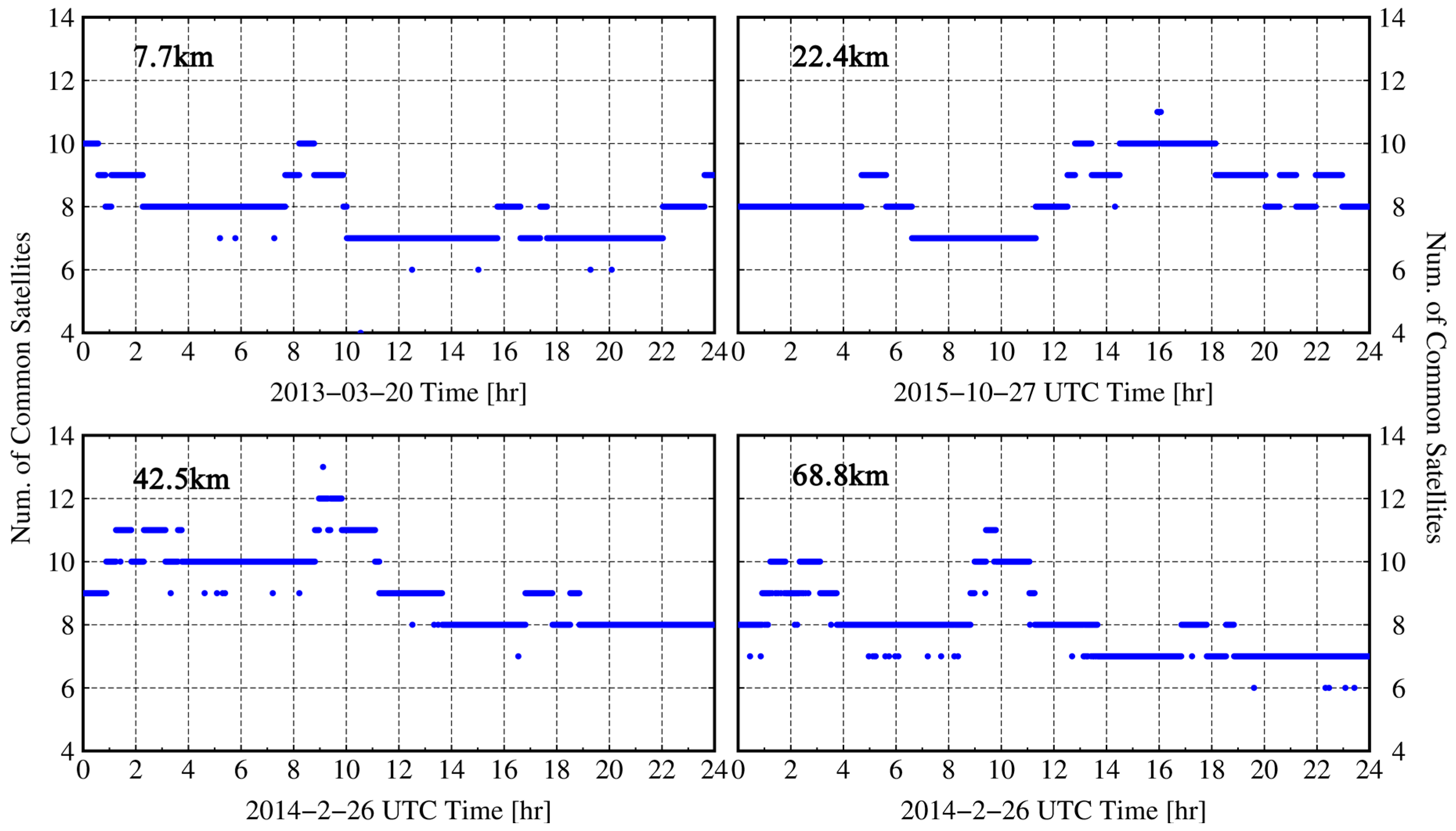
In order to test the proposed TCAR method, a series of actual triple-frequency BDS data were collected. The baseline distances of the selected stations vary from 7.7 km to 68.8 km. Table 2 gives a summary of the data including the baseline distance, the time of data collection and the sampling rate. The distribution of these stations is shown in Figure 1. The number of common satellites for four baselines is also given in Figure 2. To evaluate the ambiguity resolution performance later, we correctly resolve the NL ambiguities among three frequencies beforehand using the whole span of data. The stations of CUT0, PERT and JFNG belong to the international GNSS service (IGS) network, whose locations are being precisely known. In contrast, the precisely locations of WUDH, WHHP, and WHHN cannot be publicly obtained. We use the commercial post-processing software (NovAtel GrafNav) to obtain the coordinate of these stations, i.e., the precise point positioning (PPP) mode using the IGS precise products. Moreover, because the WL and NL model from the proposed TCAR method contain the non-dispersive terms, the tropospheric bias needs to be taken into account. The hydrostatic part of tropospheric delay contained in the un-differenced observations is compensated by the Saastamoinen model [26]. The wet part of troposphere delay is estimated by zenith wet parameter along with Niell mapping function [27]. The parameter is assumed to be a random-walk process [6,28]. The corresponding state transition between two consecutive epochs is τk = τk−1 + ω, in which ω denotes the process noise with the corresponding variance σω2 = qτ ∆t, where qτ and ∆t is the spectrum density coefficients and the sampling internal, respectively. We take qτ = 3 cm2/h for tropospheric estimated model [6]. In addition, the cutoff elevation angle is set to 15°. The elevation-dependent weighting is applied, and the observation STD at elevation θ is σ(θ) = σo(1 + 1/sin(θ))with σo being the STD in zenith, which takes 30 cm and 3 mm for triple-frequency un-differenced code and phase observation, respectively. Moreover, in order to further improve estimated precision and efficiency, we use the sequential method of the extended Kalman filter as introduced in [6].
3.2. Error Analysis of the Combined Observation
In order to validate the performance of the proposed TCAR method with respect to different ionospheric cases, the residual double-differenced ionospheric delay is extracted using ambiguity-fixed phase observations from the proposed IFVR method.
According to the relationship of ionospheric delay between frequencies, I1, the first-order double-differenced ionospheric delay on frequency f1, can be calculated using ambiguity-corrected observation and . It can be expressed as
Figure 3 shows the calculated results of the ionospheric delay on frequency f1, in which the different color codes represent the ionospheric delay from each satellite-pairs. It can be found from Figure 3 that, the peaks of the ionospheric delay for the baseline distance of 7.7 km, 22.4 km, 42.5 km, and 68.8 km can reach up to 11.6 cm, 18.1 cm, 58.0 cm, and 72.4 cm, respectively. It should be pointed out that the ionospheric delay for 68.8 km can be up to 3.8 cycles with respect to the wavelength of f1. It is because the ionospheric delay does not only depend on the baseline distance but also the ionospheric condition. The peak of ionospheric delay fluctuations for the 68.8 km is at the local time from 18:00 to 22:00, which correspond to the local sunset and midnight. This relatively large ionospheric delay is probably related to the ionospheric disturbance, i.e., the so-called traveling ionospheric disturbances (TID) [29]. Because the new ionosphere-free combinations are used in the proposed TCAR method, the ambiguity resolution will not be affected by the ionospheric bias.
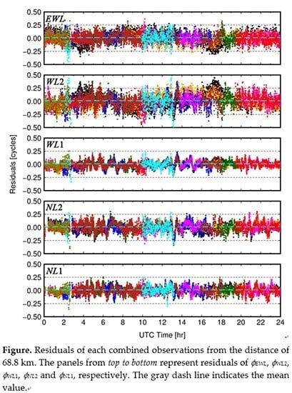
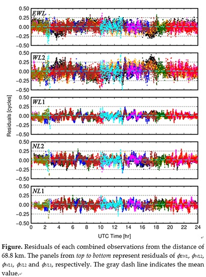
In addition to the effect of ionospheric bias, the combined observation noise is another factor impacting the reliability of ambiguity resolution. Because the residuals of observation reflect the noise level of observation, we therefore use Figure 4 to show different combined observation residuals with respect to each visible satellites-pair for the baseline of 68.8 km. It can be seen that the majority of observation residuals can be restricted to within 0.25 cycles and the mean is close to 0 cycles. This demonstrates that the proposed TCAR method is not only capable of eliminating the effect of atmospheric bias, but also can restrict the noise level, which has a positive effect on the fast and reliable ambiguity resolution. The statistical results of residuals for all baselines are listed in Table 3. It can be seen that the maximum of STD of observation residuals are less than 0.15 cycles. Moreover, it can be found that the residual level of φWL2 and φEWL are larger than that of the others. This is because these two combined observations are constructed by using code observation with low precision. However, the STD of the residuals of these two combinations can still be restricted within 0.15 cycles, which means the reliable ambiguity resolution can be achieved.
3.3. Performance of Ambiguity Resolution
In order to demonstrate the effectiveness of the proposed TCAR method (denoted as the IFVR), two ‘state-of-the-art’ methods, namely, the geometry-based and ionosphere-reduced TCAR method (denoted as the GBIR, referred to by [4]) and the geometry-free and ionosphere-free TCAR method (denoted as the GFIF, referred to by [17]) are selected to be compared. The GBIR is selected to demonstrate the effectiveness of eliminating ionospheric bias for reliable ambiguity resolution. The method constructs the three EWL, WL, and NL ambiguities, which selects the combined strategies as follows: EWL (φ(0,−1,1), p(0,1,1)), WL(φ(1,4,−5), ), and NL(φ(4,−3,0), ) referred to by [4,30]. In addition, the comparison between GFIF and IFVR is made to demonstrate the necessity of restricting the combinational noise level. The method consists of three cascaded steps, whose combined observations for each step are selected as EWL (φ(0,−1,1) − p(0,1,1)), WL (φ(1,4,−5) − p(1,1,1)), and NL (a1 + a2 − φ(1,0,0)), of which a is corresponding combined factors, referred to by [7,17]. Note that the LAMBDA algorithm is used for the ambiguity resolution of IFVR, GFIF, and GBIR, in which the threshold value for the ratio test is set to 3. The epoch-by-epoch ambiguity resolution processing is used in order to investigate the performance of ambiguity resolution ultimately.
The experimental results are evaluated by the ambiguity resolution performance and positioning accuracy. The ambiguity resolution performance of EWL, WL and NL steps are shown by the metrics of the empirical fixed rate (Pfix) and the conditional success rate (Pcf), in which Pfix are defined as the ratio between the epochs of the ambiguity being fixed and total epochs, and Pcf is defined as the ratio between the epochs of the ambiguity being fixed correctly and the epochs of the ambiguity being fixed, in which the ambiguity can been accepted as fixed only if the ratio-test is passed. Herein, Pfix reflects the continuity of ambiguity resolution, while Pcf reflects the correctness of ambiguity resolution. As discussed in [21,31], the empirical fixed rate and conditional success rate reflects the reliability of ambiguity resolution, which are listed in Table 4. The positioning errors for the three methods in the ambiguity-fixed mode are shown in Figure 5 and the corresponding STD values of positioning errors are listed in Table 5.
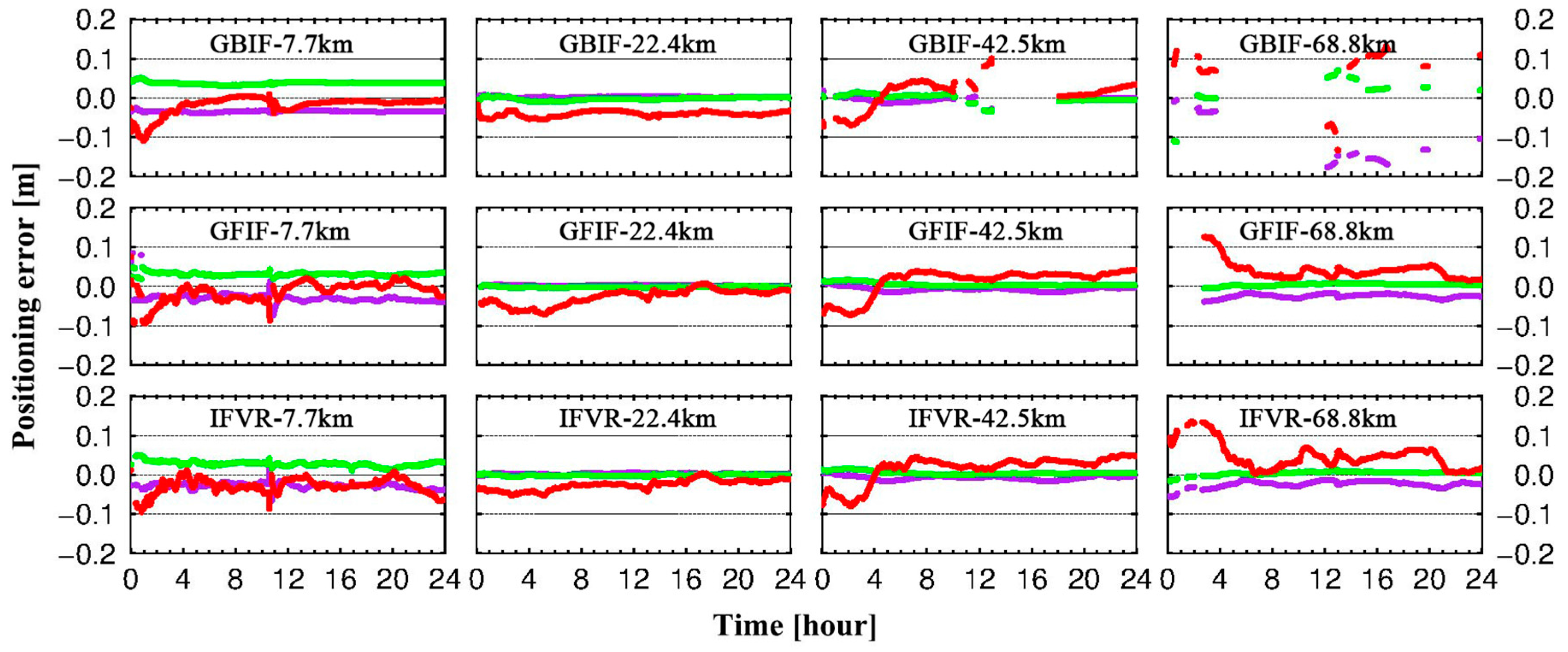
As seen from Table 4, the empirical and correctly fixed rates of EWL and WL ambiguity resolution for three methods achieve 100% regardless of the baseline distances, which reveals the effectiveness of long wavelength by observation combination. By comparing the NL ambiguity resolution result between the GBIR and the IF-based TCAR methods, i.e., the GFIF and the proposed IFVR, the necessity of the ionosphere-free combination can be demonstrated because the continuity and the reliability of GBIR is deteriorated when a larger ionospheric bias results from the increased baselines. Particularly, when the baseline increases to 68.8 km, the empirical fixed rate of GBIR is 22.5%, and the correctly fixed rate is 30.5%, respectively. Compared with the GFIF and the IFVR, it can be found that the empirical fixed rate performances are comparable to each other, which can be also be reflected by the comparable positioning accuracy performance as listed in Table 5. Note that the position error of first column is shifted from its reference value in the Figure 5. This is probably the bias from PPP-based positioning reference. However, the ambiguity resolution correctness performance of IFVR can achieve an improvement by 5.7% at most in the 68.8 km baseline distance case, which means the proposed IFVR has stronger ambiguity resolution strength than the GFIF.
4. Concluding Remarks
The purpose of this study is to improve the reliability of the TCAR method by eliminating ionospheric bias and restricting the combined observation noise simultaneously. We proposed a new ionosphere-free and combined observation variance-restricted TCAR method by utilizing ambiguity links between each step of TCAR. Since the advantage of the ambiguity link is explored sufficiently, the contradiction between the ionosphere elimination and combined observation noise suppression can be removed, so that the new ionosphere-free combination method with combined observation noise restriction can be constructed especially for WL and NL ambiguity resolution. Moreover, the strength of ambiguity resolution can also be improved by the ambiguity link, which is beneficial for improving the reliability of ambiguity resolution. The proposed TCAR method is tested using real data from various baselines. As a result, the STD of residuals of combination from each step of TCAR can be restricted within 0.15 cycles, even when the baseline is increased to 68.8 km. By comparing the NL ambiguity resolution performance of GBIR with the GFIF and the IFVR, it is found that the elimination of the effect of ionospheric bias is essential to improve the ambiguity resolution, particularly in the NL step. Meanwhile, the continuity performance is significantly improved by effectively restricting the observational noise level with respect to the wavelength, as indicated by the comparison with the GFIF and the IFVR.
Since the proposed IFVR method is capable of restricting the combined observation noise and eliminating the ionospheric bias, it is suitable for long baseline RTK positioning. The application of proposed method for 100 km or even 1000 km long baseline RTK will be our future work. In addition, the performance will be further tested with other GNSS such as GPS and Galileo.
Acknowledgments
The authors acknowledge the IGS, Xiaohong Zhang from Wuhan University (China), the GNSS Research Centre of Curtin University (Australia) for providing the BDS data. This research was jointly funded by the National Natural Science Foundation of China (No. 61773132, 61633008, 61374007, 61304235, 41674043), the Fundamental Research Funds for Central Universities (No. HEUCFP201768) and the Post-doctoral Scientific Research Foundation, Heilongjiang Province (No. LBH-Q15033).
Author Contributions
The corresponding author Liang Li proposed the research and organized the entire experimental program. Chun Jia drafted the manuscript and were responsible for field data collection. Lin Zhao, Hui Li, Jianhua Cheng and Zishen Li performed the data analysis and were involved in the writing of the manuscript.
Conflicts of Interest
The authors declare no conflict of interest.
Appendix A. Procedure for Selecting the Code Combined Coefficients
For achieving the best ambiguity resolution performance, the optimal integer coefficient for combined observations φWL2 in WL ambiguity resolution needs to follow the minimization criterion of σWL2/λWL2 = min. Assuming that the candidate integer coefficients (l,m,n) ∈ [−10,10], some optimal combined coefficient candidates can be searched with the predefined observation precision. Assuming that the standard deviations of double-differenced code and phase observations take σp = 60 cm and σφ = 6 mm, respectively, the optimal combined coefficient is (l,m,n) = (4,9,8) in mathematical analysis, in which, λWL2 ≈ 4.14 m, σWL2 ≈ 0.86 m, and then σWL2/λWL2 ≈ 0.21 cycles. However, the assumption that all code observations have the same precision does not exactly be inconsistent with the fact that the code chipping rate on f3 is 10 times faster than that of the others, which means the precision of code on frequency f3 is higher than that of the others in theoretical analysis [9,32]. Considering the difference in observation noise between p1, p2 and p3, the assumption becomes = = σp and = n·σp, in which the factor n is smaller than 1 (theoretically it is 0.1), but the practical value of 0.2 is used in this case, i.e., = = 60 cm and = 12 cm. The coefficient combination (l,m,n) = (0,0,1) can obtain a better performance with σWL2/λWL2 ≈ 0.19 cycles. Therefore, in our studies, we choose (l,m,n) = (0,0,1), considering the actual BDS environments.
Appendix B. Proof of Equivalence of IFVR and GBUC Method
We firstly introduce the equality lemma [33,34,35]. The general model can be expressed as
where, E{}, D{} denotes expectation and deviation operator, respectively; y ∈ Rn×1 is observation vector; the symbols x1 ∈ Rs×1 includes baseline, troposphere, ambiguities unknown parameters and x2 ∈ Rt×1 includes ionosphere parameters as nuisance parameters for ambiguity resolution. A1 and A2 is the corresponding design matrix, respectively. Q is covariance matrix for the observations.
In order to eliminate the nuisance parameters x2, a transition matrix C can be used to form a new observation model
Equality lemma: If the transition matrix C fulfills the condition of CA2 = 0 and rank(C) = n − t, the result can be obtained, which means the model strength of (A1) is equal as Model (A2).
The equivalence between GBUC and IFVR method can be derived by using the equality lemma.
Because the code observations p1 is not used by IFVR, therefore, the raw observations includes l={φ1, φ2, φ3, p2, p3}T, where p and φ denotes double-differenced code and phase observations, respectively, the subscript denotes the different frequency. The GBUC method is given
If the number of double-differenced satellite pairs is m, the l ∈ Rn×1, n = 5 m can be obtained; x1 = {b, τ, N1, N2, N3} ∈ R(4+3m)×1, the symbols b, τ, N denotes baseline, troposphere and ambiguity parameters, respectively; x2 = {l1} ∈ Rm×1, the symbols l represents the slant ionosphere parameters; the corresponding the design matrix is given as
with, B is design matrix of b and τ parameters, Λ = diag(λ1, λ2, λ3); μφ = [−μ1, −μ2, −μ3]T, μp = [μ2, μ3]T, where μ1 = 1, μ2 = (f1/f2)2, μ3 = (f1/f3)2; Im is identity matrix; ⊗ denotes Kronecker product.
The IFVR method formed by Equations (3), (7) and (10) can be rearranged as
where,
where, ; the coefficients a, b, c, d are defined in the Equations (5), (6) and (9). The rank (C) = n − t, which means the C is not-square matrix and is not non-singular matrix.
According to the equality lemma, the CA2 can be derived as
Therefore, the condition of CA2 = 0 and rank (C) = n − t is fulfilled between the GBUC and the IFVR method, which means the method strength of these two combinations are equivalent. However, the effectiveness of the GBUC depends on accuracy of ionospheric model, particularly, ionospheric stochastic model. In contrast, the IFVR method can be used without regard to inaccuracy of ionospheric model, which means the proposed IFVR have better ambiguity resolution performance in the presence of ionosphere.
References
- Teunissen, P.J. The least-squares ambiguity decorrelation adjustment: A method for fast GPS integer ambiguity estimation. J. Geodesy 1995, 70, 65–82. [Google Scholar] [CrossRef]
- Forssell’, B.; Martin-Neira, M.; Harrisz, R. Carrier phase ambiguity resolution in GNSS-2. In Proceedings of the 10th International Technical Meeting of the Satellite Division of The Institute of Navigation (ION GPS 1997), Kansas City, MO, USA, 16–19 September 1997; pp. 1727–1736. [Google Scholar]
- Vollath, U.; Birnbach, S.; Landau, L.; Fraile-Ordoñez, J.M.; Martí-Neira, M. Analysis of Three-Carrier Ambiguity Resolution Technique for Precise Relative Positioning in GNSS-2. Navigation 1999, 46, 13–23. [Google Scholar] [CrossRef]
- Feng, Y. GNSS three carrier ambiguity resolution using ionosphere-reduced virtual signals. J. Geodesy 2008, 82, 847–862. [Google Scholar] [CrossRef]
- Henkel, P.; Günther, C. Reliable Integer Ambiguity Resolution: Multi-Frequency Code Carrier Linear Combinations and Statistical A Priori Knowledge of Attitude. Navigation 2012, 59, 61–75. [Google Scholar] [CrossRef]
- Li, B.; Feng, Y.; Gao, W.; Li, Z. Real-time kinematic positioning over long baselines using triple-frequency BeiDou signals. IEEE Trans. Aerosp. Electron. Syst. 2015, 51, 3254–3269. [Google Scholar] [CrossRef]
- Chen, D.; Ye, S.; Xia, J.; Liu, Y.; Xia, P. A geometry-free and ionosphere-free multipath mitigation method for BDS three-frequency ambiguity resolution. J. Geodesy 2016, 90, 703–714. [Google Scholar] [CrossRef]
- Cocard, M.; Bourgon, S.; Kamali, O.; Collins, P. A systematic investigation of optimal carrier-phase combinations for modernized triple-frequency GPS. J. Geodesy 2008, 82, 555–564. [Google Scholar] [CrossRef]
- Tang, W.; Deng, C.; Shi, C.; Liu, J. Triple-frequency carrier ambiguity resolution for Beidou navigation satellite system. GPS Solut. 2014, 18, 335–344. [Google Scholar] [CrossRef]
- Li, B.; Verhagen, S.; Teunissen, P.J. Robustness of GNSS integer ambiguity resolution in the presence of atmospheric biases. GPS Solut. 2014, 18, 283–296. [Google Scholar] [CrossRef]
- Sieradzki, R.; Paziewski, J. Study on reliable GNSS positioning with intense TEC fluctuations at high latitudes. GPS Solut. 2016, 20, 553–563. [Google Scholar] [CrossRef]
- Sieradzki, R.; Paziewski, J. MSTIDs impact on GNSS observations and its mitigation in rapid static positioning at medium baselines. Ann. Geophys. 2016, 58, 0661. [Google Scholar]
- Wang, K.; Rothacher, M. Ambiguity resolution for triple-frequency geometry-free and ionosphere-free combination tested with real data. J. Geodesy 2013, 87, 539–553. [Google Scholar] [CrossRef]
- Li, J.; Yang, Y.; He, H.; Guo, H. An analytical study on the carrier-phase linear combinations for triple-frequency GNSS. J. Geodesy 2017, 91, 151–166. [Google Scholar] [CrossRef]
- Odijk, D. Ionosphere-free phase combinations for modernized GPS. J. Surv. Eng. 2003, 129, 165–173. [Google Scholar] [CrossRef]
- Richert, T.; El-Sheimy, N. Optimal linear combinations of triple frequency carrier phase data from future global navigation satellite systems. GPS Solut. 2007, 11, 11–19. [Google Scholar] [CrossRef]
- Li, B.; Feng, Y.; Shen, Y. Three carrier ambiguity resolution: Distance-independent performance demonstrated using semi-generated triple frequency GPS signals. GPS Solut. 2010, 14, 177–184. [Google Scholar] [CrossRef]
- Teunissen, P. On the sensitivity of the location, size and shape of the GPS ambiguity search space to certain changes in the stochastic model. J. Geodesy 1997, 71, 541–551. [Google Scholar] [CrossRef]
- Geng, J.; Bock, Y. Triple-frequency GPS precise point positioning with rapid ambiguity resolution. J. Geodesy 2013, 87, 449–460. [Google Scholar] [CrossRef]
- Zhao, Q.; Dai, Z.; Hu, Z.; Sun, B.; Shi, C.; Liu, J. Three-carrier ambiguity resolution using the modified TCAR method. GPS Solut. 2015, 19, 589–599. [Google Scholar] [CrossRef]
- Li, L.; Jia, C.; Zhao, L.; Yang, F.; Li, Z. Integrity monitoring-based ambiguity validation for triple-carrier ambiguity resolution. GPS Solut. 2017, 21, 797–810. [Google Scholar] [CrossRef]
- Liu, L.; Wan, W.; Ning, B.; Pirog, O.; Kurkin, V. Solar activity variations of the ionospheric peak electron density. J. Geophys. Res. Space Phys. 2006, 111. [Google Scholar] [CrossRef]
- Misra, P.; Enge, P. Global Positioning System: Signals, Measurements and Performance, 2nd ed.; Ganga-Jamuna Press: Lincoln, MA, USA, 2006. [Google Scholar]
- Urquhart, L. An Analysis of Multi-Frequency Carrier Phase Linear Combinations for GNSS; Technical Report No. 263; Universtiy of New Brunswick: Fredericton, NB, Canada, 2009. [Google Scholar]
- Joosten, P.; Teunissen, P.J.; Jonkman, N. GNSS three carrier phase ambiguity resolution using the LAMBDA-method. Proc. GNSS 1999, 99, 5–8. [Google Scholar]
- Saastamoinen, J. Contributions to the theory of atmospheric refraction. Bull. Géodésique (1946–1975) 1973, 107, 13–34. [Google Scholar] [CrossRef]
- Niell, A. Global mapping functions for the atmosphere delay at radio wavelengths. J. Geophys. Res. Solid Earth 1996, 101, 3227–3246. [Google Scholar] [CrossRef]
- Wielgosz, P.; Paziewski, J.; Baryła, R. On constraining zenith tropospheric delays in processing of local GPS networks with Bernese software. Surv. Rev. 2011, 43, 472–483. [Google Scholar] [CrossRef]
- Ding, F.; Wan, W.; Xu, G.; Yu, T.; Yang, G.; Wang, J.S. Climatology of medium-scale traveling ionospheric disturbances observed by a GPS network in central China. J. Geophys. Res. Space Phys. 2011, 116. [Google Scholar] [CrossRef]
- Zhang, X.; He, X. Performance analysis of triple-frequency ambiguity resolution with BeiDou observations. GPS Solut. 2016, 20, 269–281. [Google Scholar] [CrossRef]
- Li, L.; Li, Z.; Yuan, H.; Wang, L.; Hou, Y. Integrity monitoring-based ratio test for GNSS integer ambiguity validation. GPS Solut. 2016, 20, 573–585. [Google Scholar] [CrossRef]
- Montenbruck, O.; Hauschild, A.; Steigenberger, P.; Hugentobler, U.; Teunissen, P.; Nakamura, S. Initial assessment of the COMPASS/BeiDou-2 regional navigation satellite system. GPS Solut. 2013, 17, 211–222. [Google Scholar] [CrossRef]
- Schaffrin, B.; Grafarend, E. Generating classes of equivalent linear models by nuisance parameter elimination. Manuscr. Geod. 1986, 11, 262–271. [Google Scholar]
- Shen, Y.; Xu, G. Simplified equivalent representation of GPS observation equations. GPS Solut. 2008, 12, 99–108. [Google Scholar] [CrossRef]
- Li, B.; Ge, H.; Shen, Y. Comparison of Ionosphere-free, Uofc and Uncombined PPP Observation Models. Acta Geod. Cartogr. Sin. 2015, 44, 734–740. [Google Scholar]
Figure 1.
Distribution of the selected stations in our experiment.
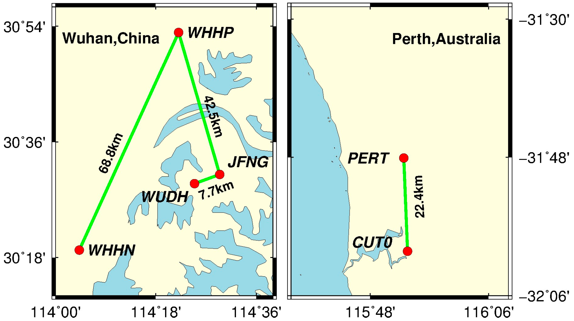
Figure 2.
Number of common satellites for four baselines. Top left: 7.7 km, Top right: 22.4 km, Bottom left: 42.5 km, Bottom right: 68.8 km.
Figure 2.
Number of common satellites for four baselines. Top left: 7.7 km, Top right: 22.4 km, Bottom left: 42.5 km, Bottom right: 68.8 km.

Figure 3.
Double-differenced ionospheric delay on frequency f1 for four baselines. Top left: 7.7 km, Top right: 22.4 km, Bottom left: 42.5 km, Bottom right: 68.8 km.
Figure 3.
Double-differenced ionospheric delay on frequency f1 for four baselines. Top left: 7.7 km, Top right: 22.4 km, Bottom left: 42.5 km, Bottom right: 68.8 km.
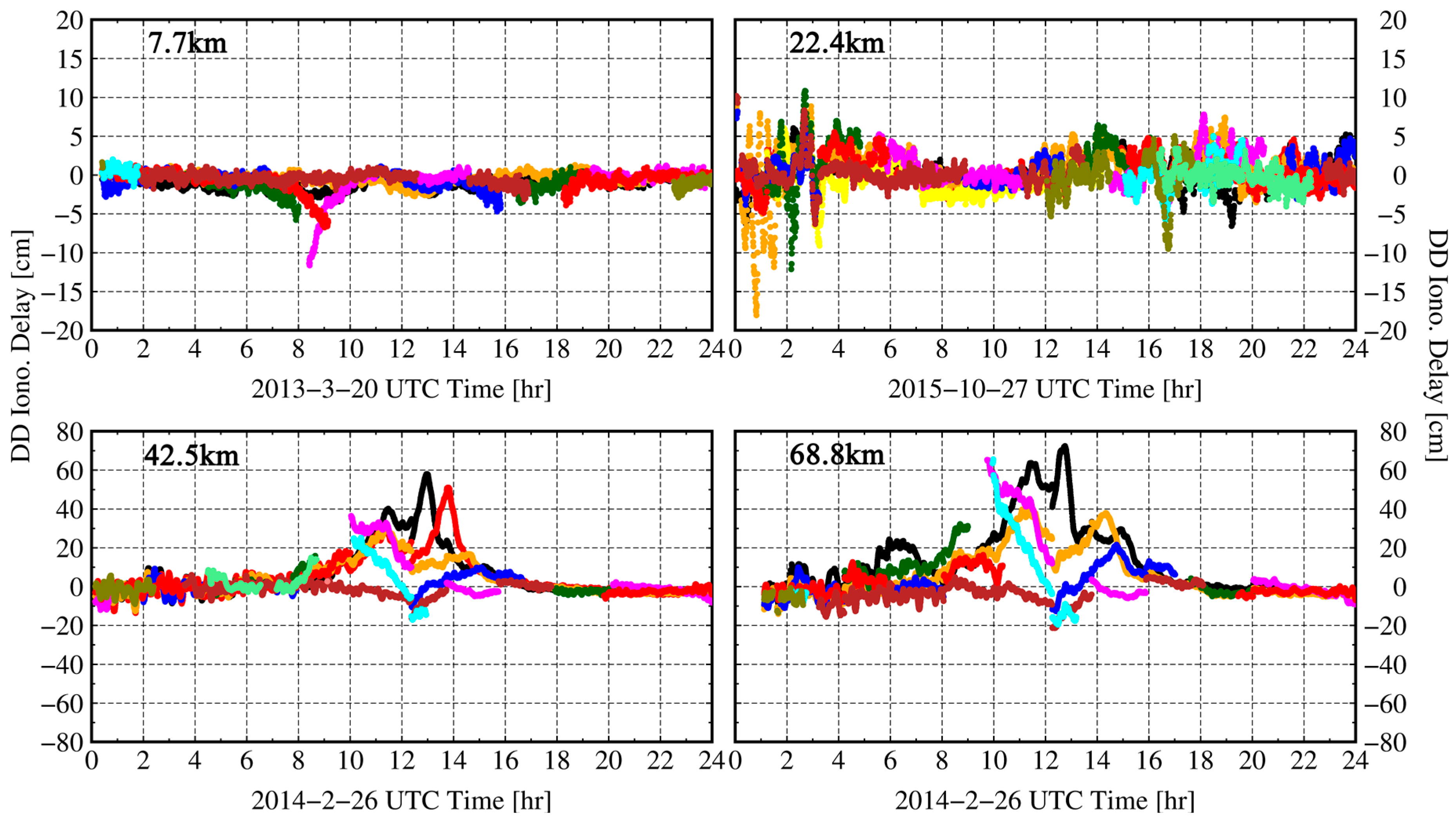
Figure 4.
Residuals of each combined observations from the distance of 68.8 km. The panels from top to bottom represent residuals of φEWL, φWL2, φWL1, φNL2 and φNL1, respectively. The gray dash line indicates the mean value.
Figure 4.
Residuals of each combined observations from the distance of 68.8 km. The panels from top to bottom represent residuals of φEWL, φWL2, φWL1, φNL2 and φNL1, respectively. The gray dash line indicates the mean value.
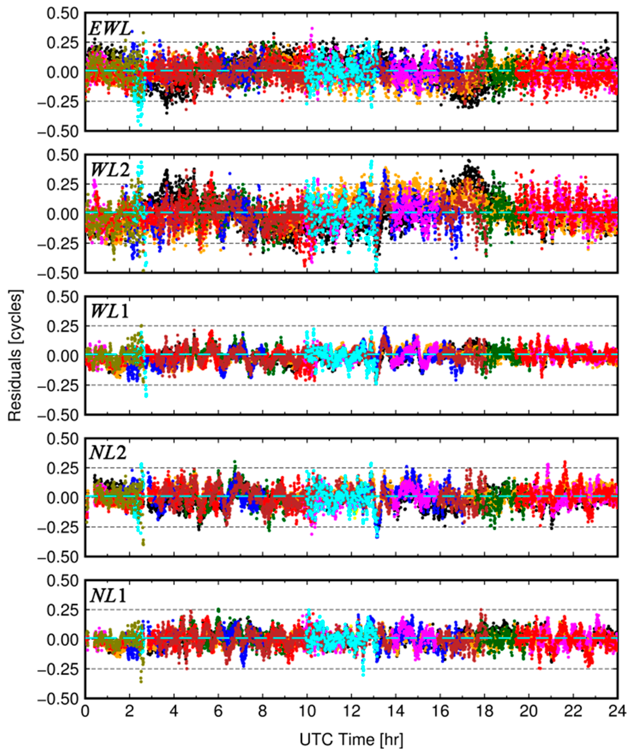
Figure 5.
Positioning error comparison for different methods in the ambiguity-fixed mode. The row panels from top to bottom denote GBIR, GFIF, and IFVR, respectively. The column panels from left to right denote the distances of 7.7 km, 22.4 km, 42.5 km, and 68.8 km. The colors of purple, green and red represent the positioning errors in the east, north, and up components, respectively.


Table 1.
Coefficients for the extra-wide-lane (EWL), (wide-lane) WL, and narrow-lane (NL) observations of the proposed ionosphere-free and variance-restricted (IFVR) method.
Table 1.
Coefficients for the extra-wide-lane (EWL), (wide-lane) WL, and narrow-lane (NL) observations of the proposed ionosphere-free and variance-restricted (IFVR) method.
| Observations | Combination |
|---|---|
| φEWL | |
| φWL1 | |
| φWL2 | |
| φNL1 | |
| φNL2 |
Table 2.
Data information.
| No. | Dis. | UTC | Duration | Interval(s) |
|---|---|---|---|---|
| 1 | 7.7 km | 2013/3/20 | 24 h | 30 |
| 2 | 22.4 km | 2015/10/27 | 24 h | 30 |
| 3 | 42.5 km | 2014/2/26 | 24 h | 30 |
| 4 | 68.8 km | 2014/2/26 | 24 h | 30 |
Table 3.
Statistics of residuals for each combined observation from all of data (STD: cycles).
| Dis. | φNL1 | φNL2 | φWL1 | φWL2 | φEWL |
|---|---|---|---|---|---|
| 7.7 km | 0.05 | 0.06 | 0.03 | 0.10 | 0.09 |
| 22.4 km | 0.06 | 0.08 | 0.04 | 0.13 | 0.10 |
| 42.5 km | 0.06 | 0.07 | 0.05 | 0.14 | 0.10 |
| 68.8 km | 0.06 | 0.07 | 0.06 | 0.12 | 0.09 |
Table 4.
Ambiguity validation performances for different methods (×100%).
| Amb. | Dis. | GBIR | GFIF | IFVR | |||
|---|---|---|---|---|---|---|---|
| Pfix | Pcf | Pfix | Pcf | Pfix | Pcf | ||
| EWL | 7.7 km | 100 | 100 | 100 | 100 | 100 | 100 |
| 22.4 km | 100 | 100 | 100 | 100 | 100 | 100 | |
| 42.5 km | 100 | 100 | 100 | 100 | 100 | 100 | |
| 68.8 km | 100 | 100 | 100 | 100 | 100 | 100 | |
| WL | 7.7 km | 100 | 100 | 100 | 100 | 100 | 100 |
| 22.4 km | 100 | 100 | 100 | 100 | 100 | 100 | |
| 42.5 km | 100 | 100 | 100 | 100 | 100 | 100 | |
| 68.8 km | 100 | 100 | 100 | 100 | 100 | 100 | |
| NL | 7.7 km | 99.1 | 99.9 | 96.6 | 99.9 | 97.6 | 99.9 |
| 22.4 km | 98.5 | 100 | 98.1 | 100 | 98.4 | 100 | |
| 42.5 km | 66.1 | 98.0 | 98.3 | 100 | 99.5 | 100 | |
| 68.8 km | 22.5 | 30.5 | 86.4 | 100 | 92.1 | 100 | |
Table 5.
Positioning errors for different methods (cm).
| Dis. | GBIR | GFIF | IFVR | |||||||||
|---|---|---|---|---|---|---|---|---|---|---|---|---|
| STD | SEP (95%) | STD | SEP (95%) | STD | SEP (95%) | |||||||
| E | N | U | E | N | U | E | N | U | ||||
| 7.7 km | 0.2 | 0.3 | 2.3 | 9.3 | 0.7 | 0.5 | 1.8 | 8.2 | 0.7 | 1.1 | 2.3 | 7.6 |
| 22.4 km | 0.2 | 0.4 | 0.7 | 5.4 | 0.2 | 0.2 | 1.3 | 4.8 | 0.1 | 0.1 | 2 | 6.4 |
| 42.5 km | 0.7 | 0.9 | 3.5 | 7.0 | 0.5 | 0.4 | 3.2 | 6.6 | 0.5 | 0.4 | 3.3 | 6.5 |
| 68.8 km | 5.9 | 3.4 | 6.2 | 20.8 | 0.5 | 0.3 | 2.3 | 11.1 | 0.8 | 0.5 | 3.6 | 12.9 |
© 2017 by the authors. Licensee MDPI, Basel, Switzerland. This article is an open access article distributed under the terms and conditions of the Creative Commons Attribution (CC BY) license (http://creativecommons.org/licenses/by/4.0/).
Share and Cite
MDPI and ACS Style
Jia, C.; Zhao, L.; Li, L.; Li, H.; Cheng, J.; Li, Z. Improving the Triple-Carrier Ambiguity Resolution with a New Ionosphere-Free and Variance-Restricted Method. Remote Sens. 2017, 9, 1108. https://doi.org/10.3390/rs9111108
AMA Style
Jia C, Zhao L, Li L, Li H, Cheng J, Li Z. Improving the Triple-Carrier Ambiguity Resolution with a New Ionosphere-Free and Variance-Restricted Method. Remote Sensing. 2017; 9(11):1108. https://doi.org/10.3390/rs9111108
Chicago/Turabian StyleJia, Chun, Lin Zhao, Liang Li, Hui Li, Jianhua Cheng, and Zishen Li. 2017. "Improving the Triple-Carrier Ambiguity Resolution with a New Ionosphere-Free and Variance-Restricted Method" Remote Sensing 9, no. 11: 1108. https://doi.org/10.3390/rs9111108
Note that from the first issue of 2016, this journal uses article numbers instead of page numbers. See further details here.