A Novel Principal Component Analysis Method for the Reconstruction of Leaf Reflectance Spectra and Retrieval of Leaf Biochemical Contents


Key Laboratory of Digital Earth Science, Institute of Remote Sensing and Digital Earth, Chinese Academy of Sciences, Beijing 100094, China
*
Author to whom correspondence should be addressed.
Remote Sens. 2017, 9(11), 1113; https://doi.org/10.3390/rs9111113
Submission received: 21 September 2017
/
Revised: 23 October 2017
/
Accepted: 24 October 2017
/
Published: 31 October 2017
(This article belongs to the Section Remote Sensing in Agriculture and Vegetation)
Abstract
:Vegetation variable retrieval from reflectance data is typically grouped into three categories: the statistical–empirical category, the physical category and the hybrid category (physical models applied to statistical models). Based on the similarities between the spectra of leaves in the optical domain, the leaf reflectance spectra can be linearly modelled using a very limited number of principal components (PCs) if the PCA (principal component analysis) transformation is carried out at the sample dimension. In this paper, we present a novel data-driven approach that uses the PCA transformation to reconstruct leaf reflectance spectra and also to retrieve leaf biochemical contents. First, the PCA transformation was carried out on a training dataset simulated by the PROSPECT-5 model. The results showed that the leaf reflectance spectra can be accurately reconstructed using only a few leading PCs, as the ten leading PCs contained 99.999% of the total information in the 3636 training samples. The spectral error between the simulated or measured reflectance and the reconstructed spectra was also investigated using the simulated and measured datasets (ANGERS and LOPEX’93). The mean root mean squared error (RMSE) values varied from 5.56 × 10⁻⁵ to 6.18 × 10⁻³, which is about 3–10 times more accurate than the PROSPECT simulation method for measured datasets. Secondly, the relationship between PCs and leaf biochemical components was investigated, and we found that the PCs are closely related to the leaf biochemical components and to the reflectance spectra. Only when the weighting coefficient of the most sensitive PC was employed to retrieve the leaf biochemical contents, the coefficients of determination for the PCA data-driven model were 0.69, 0.99, 0.94 and 0.68 for the specific leaf weight (SLW), equivalent water thickness (EWT), chlorophyll content (Cab) and carotenoid content (Car), respectively. Finally, statistical models for the retrieval of leaf biochemical contents were developed based on the weighting coefficients of the sensitive PCs, and the PCA data-driven models were validated and compared to the traditional VI-based and physically-based approaches for the retrieval of leaf properties. The results show that the PCA method shows similar or better performance in the estimation of leaf biochemical contents. Therefore, the PCA method provides a new and accurate data-driven method for reconstructing leaf reflectance spectra and also for retrieving leaf biochemical contents.
1. Introduction
Remote sensing of canopy biophysical variables is important in many applications ranging from precision agriculture [1,2] to global assessments of the carbon and nutrient cycles [3,4,5]. Vegetation variable retrievals from remote sensing data are typically grouped in three categories: the statistical–empirical category, the physical category, and the hybrid category (physical models applied to statistical models) [5,6,7].
The statistical–empirical method is typically based on a regression function that links measured biochemical or biophysical parameters to spectral measurements [7,8], such as spectral reflectance [9,10], spectral indices [11,12,13,14], red-edge features [15,16,17,18], absorption features [19,20,21,22], and band combinations made using the wavelet transformation or principal transformation [23,24,25,26]. However, the leaf spectrum depends on a complex interaction between internal and external factors that may vary significantly from one species to another, and it is hard to build a universal relationship between a single vegetation variable and a spectral signature [27].
The physically-based radiation-transfer models (RTM) have proved to be a promising alternative as they describe the radiation transfer within a leaf or canopy based on physical laws and thus provide an explicit connection between the biophysical variables and the canopy reflectance [28]. Various strategies have been proposed for the inversion of the vegetation RTMs, including numerical optimization approaches [29,30,31], and look-up table approaches [32,33,34]. Some hybrid inversion methods were also developed using both statistical and physically-based methods to retrieve vegetation parameters, such as artificial neural network approaches [35,36,37,38], and machine learning regression algorithms [39,40,41,42,43]. Verrelst et al. used ANN, SVM, kernel ridge regression (KRR), and Gaussian process regression (GPR) methods to predict LAI and concluded that GPR was a fast and accurate nonlinear retrieval algorithm [39]. The main limitation of using RTMs is the ill-posed nature of the model inversion which arises because different combinations of leaf parameters may correspond to very similar spectra [30]. This makes the choice of the initial parameter values important, and some regularization of the inverse problem may be required, implying the use of a priori knowledge to constrain the inversion process [30,34]. Ground measurements acquired during field campaigns are key to validating remote sensing estimates. Numerous methods were presented to collect ground-based measurements, while there may be some differences and uncertainties among these methods even for one variable, such as leaf area index (LAI) [44,45,46].
Principal component analysis (PCA) is a statistical procedure that uses an orthogonal transformation to convert a set of observations of possibly correlated variables into a set of values of linearly uncorrelated variables called principal components (PCs). In the field of hyperspectral remote sensing, the PCA method is usually carried out at the spectral dimension, and the PCs are normally computed as the transform of spectral measurements made at different wavelengths into an orthogonal system of eigenvectors. Generally, due to the high degree of spatial similarity between different bands, most of the variation in the data set can be explained by only a few leading PCs (if the PCA transformation is done at the spectral dimension), which can be used to represent the original observations. The PCA method is widely used in dimensionality reduction (DR) and has several applications in hyperspectral image analysis, including denoising [47], spectral unmixing [48] and target detection [49]. Besides, various alternative DR methods have been also presented [43]. For example, Rivera-Caicedo et al. evaluated 11 DR methods in combination with advanced machine learning regression algorithms (MLRAs) for statistical variable retrieval [43].
Furthermore, PCA methods are also used for selecting subsets of variables used in regression equations of surface properties such as the leaf area index (LAI) [23,50,51,52,53,54,55,56,57], canopy chlorophyll content [24,58,59], soil properties [60] and the chlorophyll concentration of inland water bodies [61,62]. Some hyperspectral studies have demonstrated that regression models using PCA (over spectral dimension) gave superior results as compared to using VIs [23,50,51,52,53,59]. For example, Satapathy showed that the retrieved LAI from PCA has higher accuracy (RMSE = 0.137) than the classical NDVI–LAI empirical approach (RMSE = 1.139) [51]. Chaurasia and Dadhwal found that a multi-band PCA inversion approach yielded a high accuracy (RMSE = 0.380) as compared to NDVI and SR approaches (RMSE = 2.28, 0.88) [50]. Partial least squares regression (PLSR) is a multiple linear regression method that concentrates the merits of multiple linear regression analysis and principal component analysis [57]. PLSR is also a PCA data-driven approach, which does not require manual optimization. Some studies showed that PLSR performs much better than PCA in the estimation of vegetation parameters [57,58]. However, other hyperspectral studies showed that such a PCA method did not show better performance than the VI-based method [54,55,56,57]. For example, Gonsamo et al. found that the estimated LAI from the NDVI-based model significantly correlated with the ground-measured LAI with a R2 of 0.63 and RMSE of 0.52, while the LAI inverted from the PCA method showed poor correlation with ground-measured LAI [54]. Ray et al. found that none of the principal components (PCs) showed significant correlation with LAI while some VIs correlate well with LAI [55]. This might be due to the fact that the PCs provide only statistical measures, whereas the other indices are based on a priori knowledge of the connections between specific physiological and reflectance features [55]. By definition, the components are dependent on the covariance of the training dataset. That means that a regression model based on single or multi-band component(s) is limited to being site-specific and non-transferable [50].
This high degree of spectral similarity (instead of spatial similarity) is also widely observed between reflectance or transmittance spectra of the Earth’s surface or atmosphere. For example, all green leaves show similar spectral curves that include fixed absorption features due to pigments and foliar water. Although the PCA method is good at spectral reconstruction if the PCA transform is carried out at the sample dimension, it is rarely used for this purpose. The PCA transformation was, however, used to characterize approximately 7000 downwelling solar irradiance spectra in the 380–1700 nm region at the sample dimension in a study by Rabbette and Pilewskie [63]; it was found that the first four PCs accounted for the spectral variability due to column-integrated liquid water, water vapor, molecular scattering, and ozone, respectively. PCA has also been used to retrieve temperature and moisture profiles from high-resolution infrared satellite instruments [64]. More recently, in order to separate the subtle solar-induced chlorophyll fluorescence (SIF) from the top of atmosphere (TOA) radiance, both the atmospheric transmittance and TOA spectrum have been successfully modelled by means of a set of orthogonal PCs derived from the measured TOA spectra of non-vegetation targets (e.g., desert and cloud pixels) using the PCA transform at the sample dimension [65,66,67]. A PCA data-driven algorithm has also been developed to retrieve SO2 from OMI-measured radiance and irradiance data; this can significantly improve the quality of SO2 retrievals as compared with the current operational product [68]. In these studies on atmosphere optics, PCA is not used for data reduction, it is used to select a few linearly uncorrelated spectra to model atmosphere transmittance. Inspired by these studies, it is reasonable to assume that the leaf or canopy reflectance spectra can also be reconstructed using a few PCs if the PCA transformation was carried out at the sample dimension, and that the leaf or canopy properties can be retrieved from the weighting coefficients of PCs if the PCA transform is carried out at the sample dimension instead of the spectral dimension.
The objectives of this paper are (1) to present a PCA data-driven approach for the reconstruction of leaf reflectance spectra; (2) to investigate whether the extracted PCs are able to account for the leaf biochemical properties; (3) to present a PCA data-driven approach for the retrieval of leaf biochemical contents; and (4) to compare the performance of the PCA method for the retrieval of leaf properties with the traditional statistical–empirical or the full-physical approaches.
2. Materials and Methods
2.1. Measured and Simulated Datasets
2.1.1. LOPEX93 Dataset
The LOPEX database was established by the Joint Research Center (JRC) in 1993 and has been widely used by researchers throughout the world. In order to represent a wide range of leaf internal structure, pigmentation, and water content, plant species with different types of leaves were collected during the summer of 1993 [69]. About 70 leaf samples representative of more than 50 species were obtained from trees, crops and plants in the area near to the JRC, Ispra, Italy. The biochemical constituents include total proteins, cellulose, lignin, starch, specific leaf weight (SLW), chlorophyll and foliar water. A Perkin Elmer Lambda 19 double-beam spectrophotometer equipped with a BaSO4 integrating sphere was used for the measurement of the directional-hemisphere reflectance (R) and transmittance (T) of the upper faces of the leaves, the probe light beam of the instrument being incident on the upper face of the leaves at an angle of 8°. Spectra were collected over the 400–2500 nm region with a sampling interval of 1 nm. The spectral resolution varied from 1 to 2 nm in the visible/near infrared region (400–1000 nm) and from 4 to 5 nm in the mid-infrared (1000–2500 nm). For each sample, measurements of five different areas were made in order to quantify the small but not negligible leaf-to-leaf variability. LOPEX was originally designed to separate the cell wall constituents (lignin, cellulose, etc.) and so emphasis was placed on the measurements of dry matter and water, while the pigment measurements were averaged from five leaf samples. Therefore, the confidence in the accuracy of the chlorophyll content measurements is relatively low.
The LOPEX dataset is shared online [70].
2.1.2. ANGERS Dataset
An experiment was conducted at the INRA (National Institute for Agricultural Research) in Angers, France in June 2003 and a data set associating visible/infrared spectra of vegetation elements with physical measurements and biochemical analyses was then constructed [71]. The directional-hemisphere reflectance spectra were measured using an ASD FieldSpec spectrometer with a spectral range of 400–2500 nm and an interval of 1.4 nm. Reflectance and transmittance measurements of 276 leaf samples from 39 different species were collected along with associated biochemical and physical measurements. The biochemical parameters include leaf chlorophyll content, carotenoids, SLW and water content. The ANGERS dataset can also be accessed free online [70].
2.1.3. Simulated PROSPECT Model Dataset
The PROSPECT model is a radiative transfer model which calculates the leaf hemispherical reflectance and transmittance from 400 nm to 2500 nm [71,72]. The reflectance and transmittance spectra of the leaves are simulated using different inputs to the PROSPECT-5 model, including the structural parameter N, SLW (same as the dry matter content in many references), the chlorophyll content (Cab), the carotenoid content (Car), and the equivalent water thickness (EWT). The brown pigment of the leaf is neglected and set as zero in the simulation experiment. In this study, the PROSPECT-5 model was employed to simulate the leaf spectral data for the training and validation of the retrieval algorithm based on the principal component analysis. The focus was on retrieval of the key biochemical contents from the reflectance spectra—the inputs used in the simulation experiment are illustrated in Table 1.
The leaf biochemical parameters in Table 1 were set according to their statistical distributions in the ANGERS and LOPEX’93 datasets.
EWT was derived from leaf SLW and gravimetric water content (GWC %), as in Equation (1).
According to the statistical results of leaf biochemistries in ANGERS [71,73], the data range was 46–92% for GWC, 0.0017–0.0331 g/cm2 for SLW, and 0.0050–0.0340 cm for EWT. If leaf EWT in the PROSPECT model is assumed totally independent of SLW, its GWC may be too high for leaves with a small SLW and too low for leaves with a large SLW in some cases. In Table 1, leaf EWT is assumed with a reasonable range of GWC (50–90%) for a given SLW. Moreover, the leaves with larger SLW and GWC, as in Table 1, will still have extremely high EWT. For example, if a leaf has an SLW value of 0.02 g/cm2 and a GWC value of 90%, its leaf EWT will be 0.2 cm. This value is extremely high for natural leaves. Therefore, all the simulated samples with EWT > 0.06 cm (about twice the maximum EWT value of the ANGERS dataset) were deleted. Such assumptions were more suitable to natural cases.
Car was scaled to Cab with a ratio that varied from 1/10 to 1/2 according to the statistical results of leaf biochemistries in ANGERS [71,73].
The values of N were also linked to the SLW based on their statistical relationship. Jacquemoud and Baret [72] found that the structure parameter N is well correlated with the SLW, and they observed an increase in the SLW corresponding to an increase in the value of N. According to the ANGERS dataset [53], there is a significant relationship between N and SLW, and the empirical statistical model is listed as,
Physically, PROSPECT differentiates N and SLW [72]. Other studies show that the structure parameter N also varies with leaf internal structure and leaf water content [14,74,75]. If the structure parameter N is directly determined using the empirical model, as in Equation (2), the intrinsic variability of leaf optical properties will be underestimated. In order to account for this empirical relationship in Equation (2) and also the variability of leaf reflectance spectra, the structure parameter N of a given leaf SLW is determined by the sum of two parts. One part is the predicted item using the empirical SLW-based model as Equation (2), and the other is a random item simulated by a Gauss function with a mean value of zero and a standard deviation of 0.152, which is the root mean squared error (RMSE) of the empirical SLW-based model, as in Equation (2).
Finally, there are the 5454 simulation samples. A total of 2/3 (3636) of the samples were randomly selected as the training dataset, with the remaining samples being used as the validation dataset.
2.2. Vegetation Indices Sensitive to Leaf Biochemical Contents
A vegetation index is a non-dimensional index, usually a ratio, linear or non-linear combination of the spectral reflectance of two or more bands, which compresses important information from a hyperspectral or multispectral dataset into a vegetation index channel. Some popular spectral indices were selected for investigating and comparing the performance of the PCA method in the estimation of leaf biochemical contents. The indices used are listed in Table 2.
All these spectral indices were used to develop the statistical models for the retrieval of leaf biochemistries. Three statistical modeling methods, including a linear model, exponential model, and logarithmic model, were employed to link the spectral indices to leaf biochemistries based on the simulated training dataset. For each pair of spectral index and leaf parameters, the statistical model with the highest determination coefficient was selected as the optimal VI-based model. Then, the optimal VI-based model was validated using the validation datasets.
2.3. Principal Component Analysis
PCA methods are widely used in dimensionality reduction and have applications in hyperspectral image analysis. For most hyperspectral remote sensing applications [23,47,48,50,51,52,53,54,55,56,57,58,59,60,61,62], the PCA transformations are always conducted at the spectral dimension based on the high degree of spatial similarity between images at different bands. As illustrated in Figure 1, the spectra of leaves have similar fixed absorption features that are due to pigments and water. Therefore, based on the high degree of spectral similarity between the reflectance spectra of different leaves, it should also be possible to use PCA to reconstruct leaf spectra using a very small number of principal components by carrying out the PCA transformation at the sample dimension instead of the spectral dimension.
PCA transforms a set of original variables into a set of linearly uncorrelated variables called principal components (PCs). This transformation is defined in such a way that the first PC has the largest possible variance, and each succeeding component in turn has the highest variance possible under the constraint that it is orthogonal to the preceding components. The PCA transform can be expressed as
where is a data matrix whose columns consist of the reflectance spectra of the training samples, is the matrix containing the full PCs of the reflectance spectra of the training samples, and is a square matrix whose columns are the eigenvectors of .
Once the PCs have been determined using the training reflectance dataset, the reflectance spectrum of a leaf can be reconstructed using a linear combination of some of the leading PCs in :
where represents the leaf spectrum reconstructed by PCs, is the ith principal component, is the weight coefficient corresponding to the ith principal component, and n is the number of selected PCs.
The weight coefficients () can be retrieved using a linear least squares fitting method to minimize the error between the observed and reconstructed leaf reflectance spectra, as expressed by Equation (5):
where is the pseudoinverse of the matrix . is a column vector consisting of the observed leaf reflectance spectrum.
In this study, the aim was to investigate the relationship between the weight coefficients of different PCs and the leaf biochemical contents.
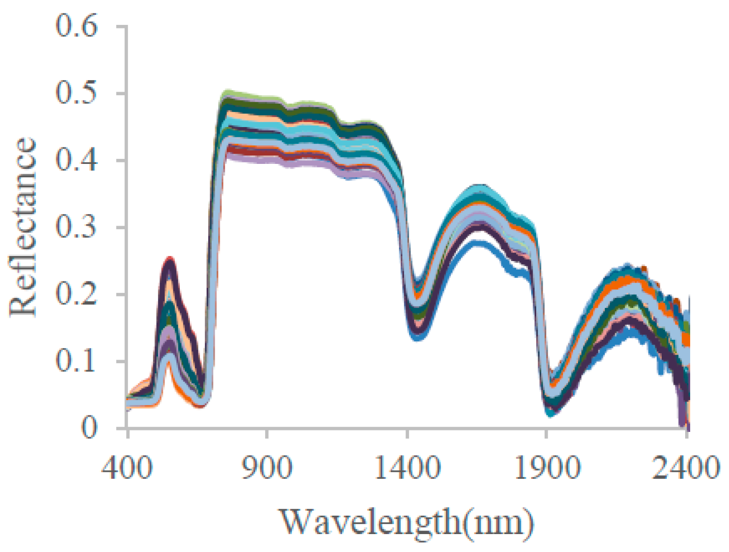
Figure 1 shows the reflectance spectra of the leaves in the ANGERS dataset. The strong absorption of light by pigments dominates green leaf properties in the visible spectrum (400–700 nm). The near-infrared plateau (NIR, 760–1300 nm) is a region where biochemical absorption is limited and the reflectance here is mainly determined by the leaf internal structure. The shortwave–infrared (SWIR, 1350–2500 nm) is a region of strong absorption, primarily by water in green leaves. Absorption by water is strongest in the spectral bands centered at 1450, 1940 and 2500 nm, with important secondary absorptions at 980 nm and 1240 nm.
As illustrated in Figure 1, a leaf reflectance spectrum is determined by the absorption of the pigments, water content, dry matter and the internal multiple scattering. In this paper, the spectral data were split into four specific datasets, each with a given spectral range over 400–2500 nm, 400–680 nm, 400–800 nm and 900–2500 nm. For datasets over 400–2500 nm, we aim to investigate the performance of the PCA method to reconstruct leaf reflectance and to retrieve leaf biochemistries; for datasets over 400–680 nm, we aim to separate the spectral contribution of Car from Cab on leaf reflectance; for datasets over 400–800 nm, we focus on retrieving Cab and at the same time eliminating the interference of the leaf EWT; for datasets over 900–2500 nm, we focus on retrieving EWT while eliminating the interference of the leaf Cab.
3. Results
3.1. Reconstruction of the Leaf Reflectance Spectra Using the PCA Data-Driven Method
Figure 2 shows the twenty leading eigenvalues of the PCs obtained using the simulated leaf reflectance spectra of the training dataset for the range 400–2500 nm. Each eigenvalue is proportional to the portion of the variance that is correlated with each eigenvector. The sum of all the eigenvalues is equal to the sum of the squared distances of the points from their multidimensional mean. It can be observed from the eigenvalues and variances that the ten leading PCs contain 99.999% of the total information. Therefore, the ten leading PCs were selected for the reconstruction of the leaf reflectance.
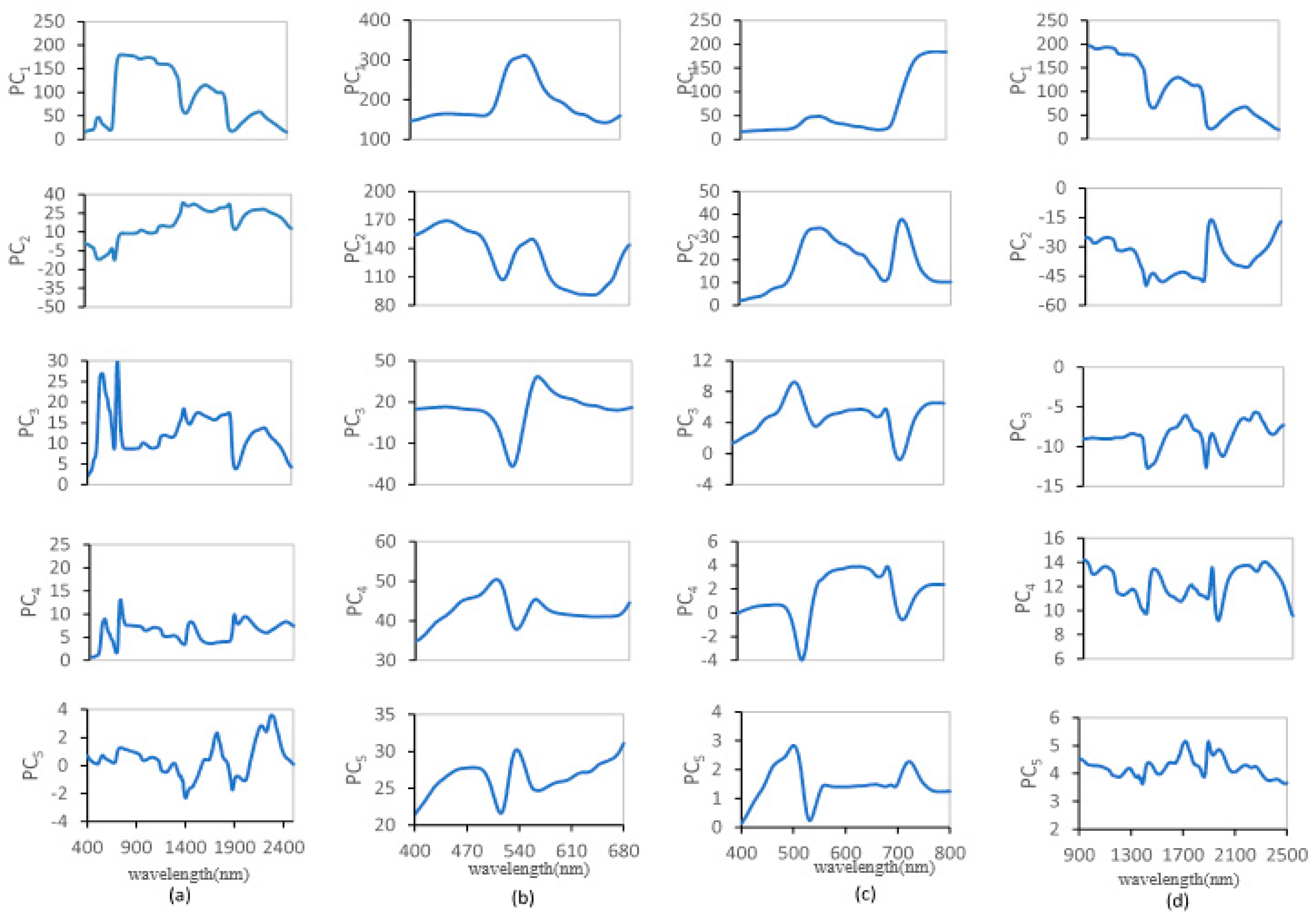
Figure 3 shows the five leading PCs of the reflectance spectra of the training dataset. These spectra were derived independently from the reflectance data for the wavelength ranges 400–2500 nm, 400–680 nm, 400–800 nm and 900–2500 nm. The first PC contains the basic shape of a reflectance spectrum, and can also describe the contribution of the leaf internal structure parameter, N, to the reflectance [73,86,87,88]. Other PCs also contain some spectral features, the specific absorption coefficients of the leaf pigments, and water content. Therefore, the weighting coefficients of the PC spectra in Equation (5) may be closely linked to the leaf biochemical contents.
Figure 4 shows the spectral RMSE between measured leaf reflectance and reconstructed reflectance using the different PCs. The results show that the spectral RMSE decreased with increased PCs, with a mean RMSE varying from 0.0499 to 0.00045 when the number of PCs increased from one to ten. When the first two PCs were employed to reconstruct the reflectance spectra, the spectral error over the SWIR region (1300–2500 nm) decreased noticeably. The spectral characteristics over the SWIR region are mainly determined by leaf EWT. Thus, the second PC could indirectly reflect the contribution of water content to leaf reflectance. When the third PC was combined with the two leading PCs to reconstruct the reflectance spectra, the spectral error over the VIS region (400–700 nm) decreased noticeably, which indicated that the third PC could indirectly reflect the contribution of pigments on leaf reflectance. Therefore, the weighting coefficients calculated using Equation (5) may be closely linked to the leaf biochemical contents.
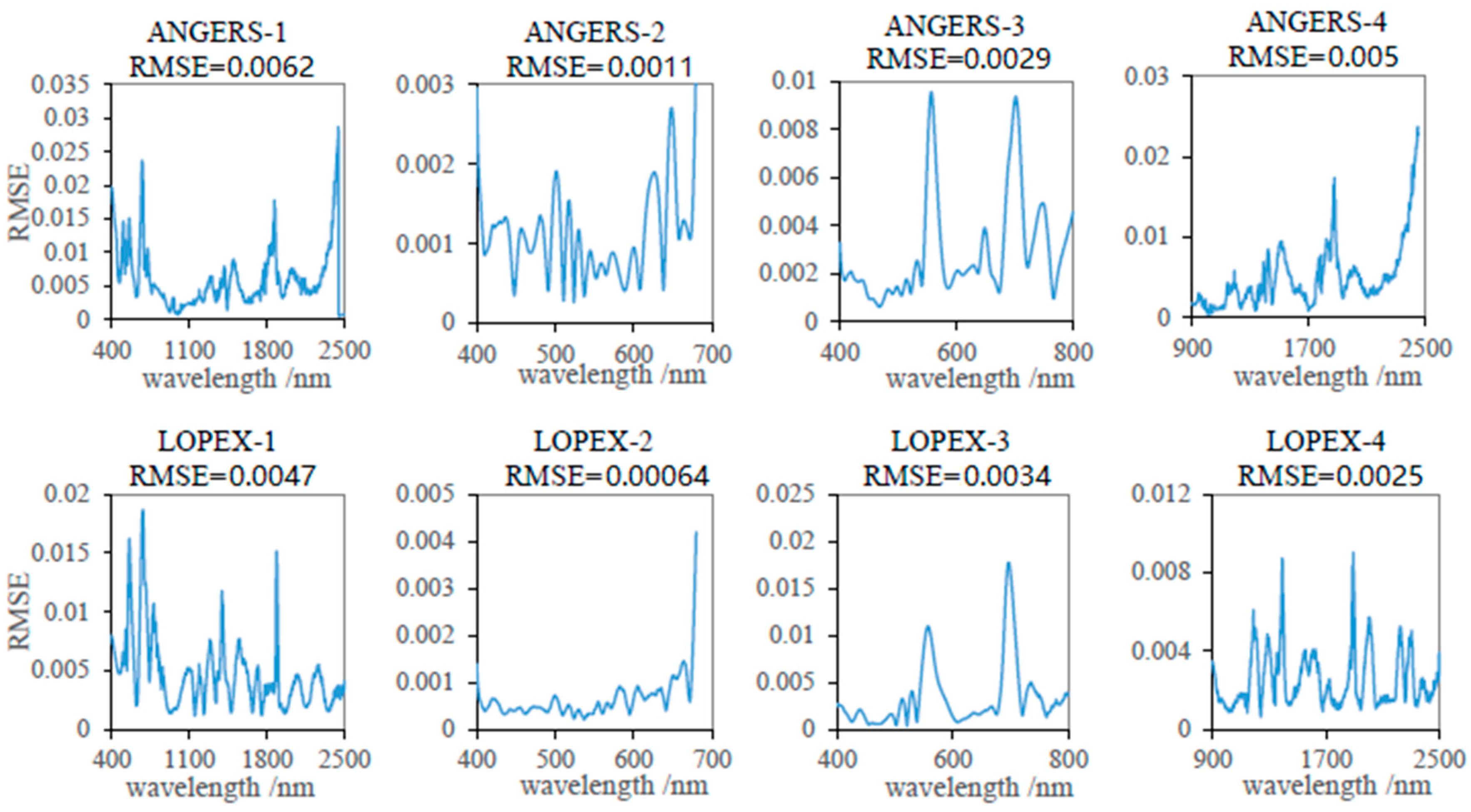
The simulated training dataset, validation dataset, ANGERS dataset and LOPEX’93 dataset were reconstructed using the ten leading PCs derived from the simulated training dataset. The mean and maximum spectral RMSE values between simulated/measured leaf reflectance and reconstructed reflectance using the PCA method are summarized in Table 3. The RMSE values of the reconstructed reflectance spectra for ANGERS and LOPEX’93 are illustrated in Figure 5. These results show that the leaf reflectance spectrum can be accurately reconstructed using the ten leading PCs—the mean RMSE varied from 5.56 × 10⁻⁵ to 6.18 × 10⁻³.
3.2. Relationship between the Weighting Coefficients of the PCs and the Leaf Biochemical Contents
As illustrated in Figure 5 and Table 3, the leaf reflectance can be accurately reconstructed using just a few leading PCs, and the spectra of some of the leading PCs are similar to the contributions of the biochemical contents to the leaf reflectance. It is also well-known that leaf spectra can be modelled using only a few leaf variables such as the SLW, water content, pigment content and a structure parameter that is used in the PROSPECT model. Therefore, the weighting coefficients of the PCs in Equation (5) can potentially be linked to the leaf biochemical contents.
The simulated training dataset was employed to examine the relationship between the weighting coefficients of the PCs and the leaf biochemical contents. The linear correlation coefficients were calculated using the least squares method to determine which PC is most sensitive to different biochemical constituents, as shown in Table 4.
According to the linear correlation coefficients listed in Table 4, the weighting coefficients of the first PC derived from the training dataset for the regions 400–2500 nm and 400–680 nm were best for the estimation of the SLW and carotenoid content, whereas the weighting coefficients of the second PC for the regions 400–800 nm and 900–2500 were best for the estimation of the chlorophyll content and EWT, respectively. These weighting coefficients were selected for the estimation of the corresponding leaf parameters.
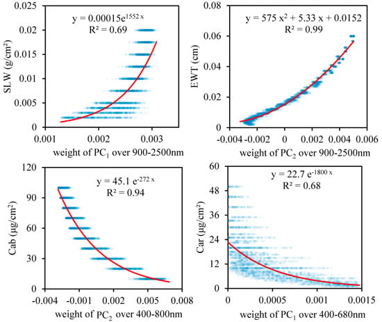
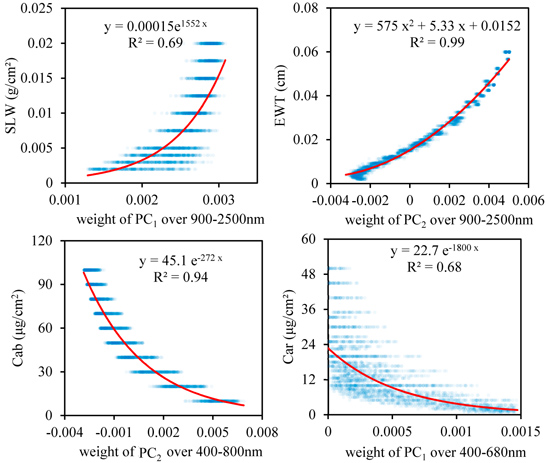
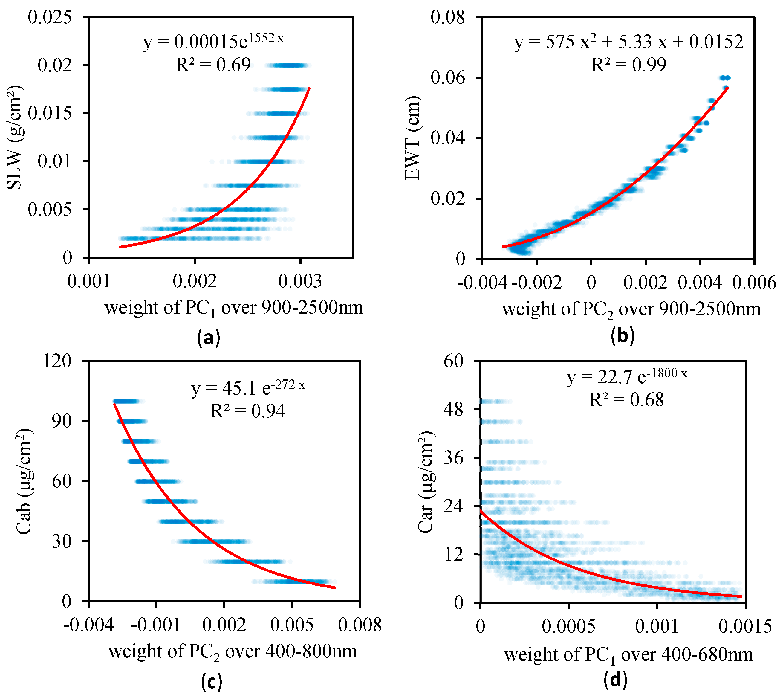
Numerous studies [79,80,85] show that the influence of leaf biochemical constituents on the reflectance and transmittance is not linear. According to scatterplots between the weighting coefficients and biochemical constituents as listed in Figure 6, an exponential model is the best expression to retrieve leaf parameters for SLW, Cab, Car, while a polynomial model is best for EWT. The statistical models for the four leaf parameters are illustrated in Figure 6; the corresponding coefficients of determination are 0.69, 0.99, 0.94 and 0.68 for the SLW, EWT, Cab and Car, respectively.
The statistical scatter plots for the SLW and Car are still a little dispersed (R2 = 0.69 and 0.68) for a reliable statistical model, which means that a single PC may be not enough to represent the values of the SLW and Car. Some combinations of the sensitive weight coefficients of PCs in Table 4 were tested for better retrieval of leaf SLW and Car. The results show that some combinations can give better performance for leaf SLW and Car.
The optimized statistical model for SLW is
where is the weighting coefficient of the corresponding, S1, S2, S3 and S4 represent the spectral regions 400–2500 nm, 400–680 nm, 400–800 nm and 900–2500 nm, j = 1, 2, …, 10 is the number of the PC.
The optimized statistical model for Car is
where is the weighting coefficient of the corresponding, S1, S2, S3 and S4 represent the spectral regions 400–2500 nm, 400–680 nm, 400–800 nm and 900–2500 nm, j = 1, 2, …, 10 is the number of the PC.
According to the statistical analysis shown in Figure 5, the statistical models for the EWT, and Cab are
where is the weighting coefficient of the second PC at 900–2500 nm, and
where is the weighting coefficient of the second PC at 400–800 nm.
3.3. Validation of the Regression Models of the Leaf Biochemical Contents
Using the regression models illustrated in Equations (6)–(9), it should be possible to retrieve the leaf biochemical parameters by a PCA transformation. These models were validated using the three validation datasets, which consisted of the simulated validation dataset, the LOPEX’93 dataset and the ANGERS dataset.
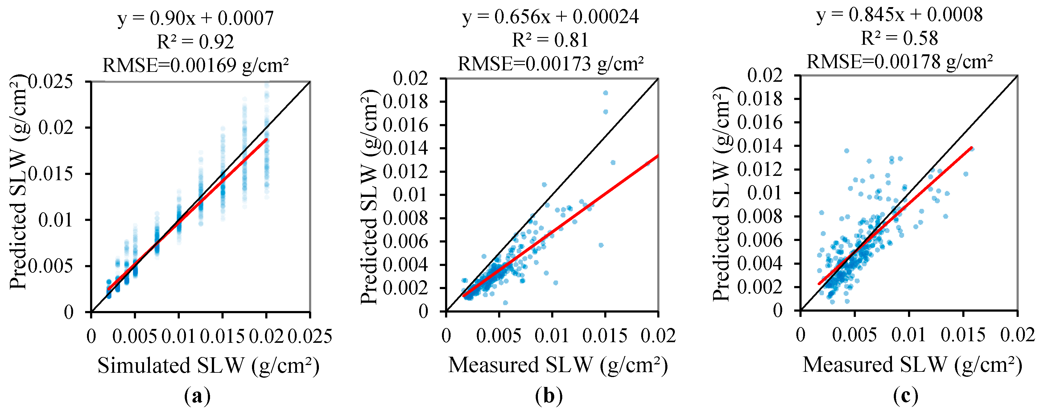
Figure 7 shows the results used to validate the SLW model as in Equation (6). The values of the RMSE were 0.00169, 0.00173, and 0.00178 g/cm2, and the coefficients of determination were 0.92, 0.81 and 0.58 for the simulated, ANGERS and LOPEX’93 datasets, respectively.
Figure 8 shows the results for the validation of the EWT model as in Equation (8). These results gave an RMSE of 0.0018, 0.0036, and 0.0028 cm, and a coefficient of determination of 0.99, 0.83 and 0.85, for the simulated validation dataset, and the ANGERS and LOPEX’93 datasets, respectively. According to scatterplot as in Figure 8, the leaf EWT was overestimated, which means that there may be some bias in the PROSPECT model to simulate the contribution of EWT to leaf reflectance.
Figure 9 shows the results for the validation of the Cab model as in Equation (9). For this model, the values of the RMSE were 7.88, 6.34, and 24.51 µg/cm2, and the coefficients of determination were 0.92, 0.92 and 0.14, for the simulated, ANGERS and LOPEX’93 datasets, respectively. Except for LOPEX’93, the samples are located close to the 1:1 line, which means that the contribution of the chlorophyll content to the leaf reflectance spectrum is well modeled using the second PC spectrum for the range 400–800 nm. LOPEX was originally designed to separate the cell wall constituents and the pigment measurements were averaged using five leaf samples. Thus, there is a lot of uncertainty about the accuracy of the chlorophyll content measurements. Therefore, despite the relatively poor results obtained in the validation of the LOPEX’93 dataset, the PCA method may still have potential for estimating chlorophyll content.
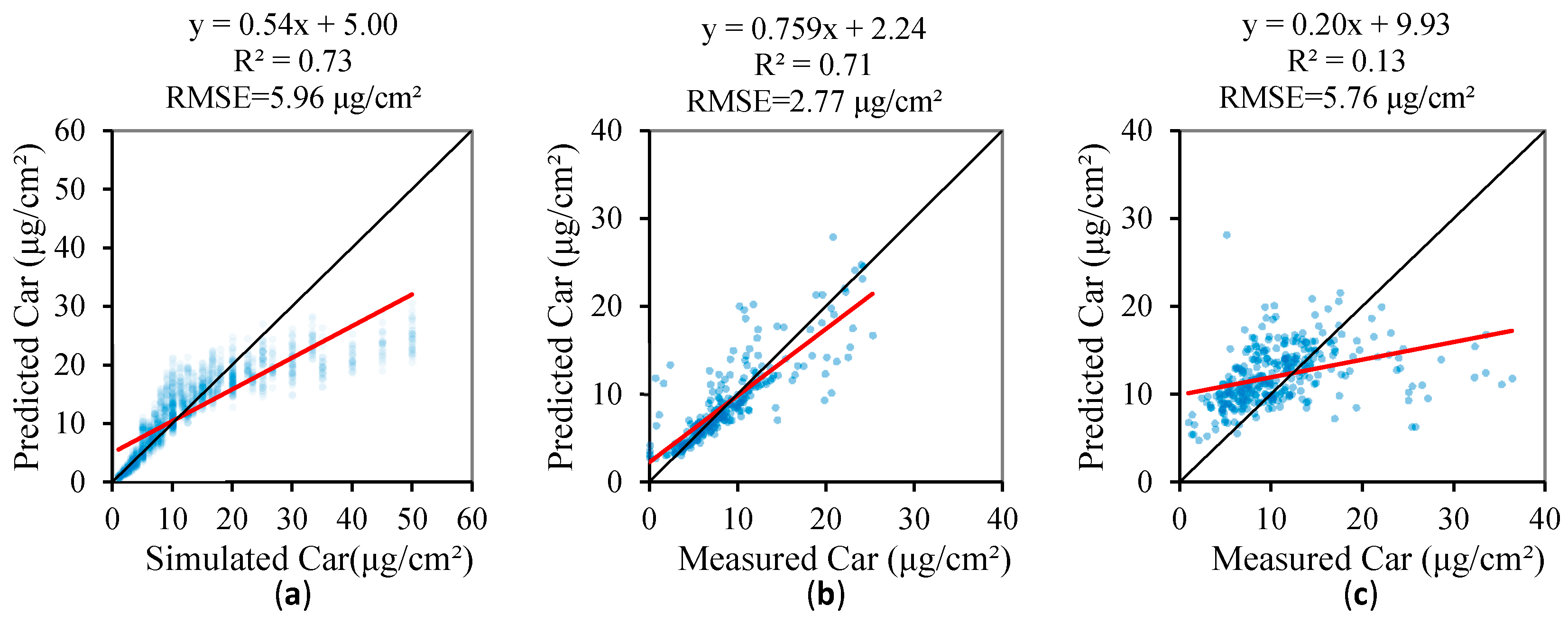
Figure 10 shows the results of the validation of the Car model as in Equation (7), which gave an RMSE of 5.96, 2.77 and 5.76 µg/cm2, and a coefficient of determination of 0.73, 0.71 and 0.13, for the simulated, ANGERS and LOPEX’93 datasets, respectively. The samples are scattered widely around the 1:1 line for all the validation datasets, which indicates that the contribution of the carotenoid content to the leaf reflectance spectrum is not well modeled by the PCA method.
3.4. Comparison of PCA Method with Traditional VI-Based Method for Retrieving Leaf Biochemical Contents
The spectral indices listed in Table 2 were employed to build the statistical models of the leaf biochemical contents using the training data simulated by the PROSPECT-5 model. The statistical models based on the simulated training dataset are listed in Table 5. The results show that some vegetation indices are significantly correlated with the leaf biochemical parameters. The most sensitive vegetation indexes are the NDMI, WI, and ND705 for the SLW, EWT and pigments, respectively.
The retrieval accuracies of the VI-based models in Table 5 were also investigated and compared to the PCA method. Three validation datasets, including the simulated validation dataset, ANGERS and LOPEX’93, were employed. The R2 and RMSE values of the most accurate VI-based models in Table 5 were summarized and compared to these metrics of the PCA method in Figure 7, Figure 8, Figure 9 and Figure 10. The validation results of the VI-based models of SLW and EWT are listed in Table 6, and the validation results of the VI-based models of Cab and Car are listed in Table 7.
The results show that:
- (1)
- the SLW can be accurately retrieved using the NDMI and NDLMA, and the PCA method also only showed similar or slightly better performance on estimation for ANGERS and LOPEX’93.
- (2)
- the EWT can be more accurately retrieved using the PCA method than those obtained using the VI-based method for all validation datasets.
- (3)
- the PCA method generally provides a better estimate of the pigment content, although the ND705–based and CIred edge–based models provide a slightly more accurate estimation for Cab when the ANGERS is used.
Therefore, the preliminary results obtained using the PCA data-driven method show that this method has the potential to produce more accurate retrievals of leaf biochemical contents than the traditional VI-based methods.
4. Discussion
4.1. The Performance of the PCA Approach in the Reconstruction of Leaf Reflectance Spectra
As shown in Figure 1, for optical observations made in the range 400 nm to 2500 nm, the leaves showed similar spectra due to fixed absorption features caused by pigments and water. Traditionally, the PCA transformation is carried out at the spectral dimension and, due to the high degree of similarity between different bands, is widely used in dimensionality reduction in hyperspectral image analysis. In this study, the PCA transformation was carried out at the sample dimension (instead of at the spectral dimension) because of the high spectral similarity between different samples. The results showed that the leaf spectrum could be accurately reconstructed and gave a mean RMSE value of 4.52 × 10⁻⁴ for the 400–2500 nm range using the simulation dataset, 6.18 × 10⁻³ using the ANGER dataset, and 4.65 × 10⁻³ using the LOPEX’93 dataset. The simulated leaf reflectance was systematically about ten times more accurately reconstructed than the measured data. This phenomenon can be attributed to two reasons. Firstly, the training data of the PCs were generated with PROSPECT-5, there is a systematic bias between PROSPECT-5 and measured reflectance. Such modelling bias cannot be totally compensated using the PCA reconstruction method. Secondly, the measurement error and noise in the measured reflectance are unavoidable, so the reconstruction accuracy for the measured data will also decrease.
The PROSPECT-5 model has been adequately evaluated and is widely used in the field of vegetation remote sensing. According to the investigations by Féret et al. [71], carried out on the CALMIT, ANGERS and HAWAII datasets, the PROSPECT-5 model resulted in an RMSE value of 0.016 to 0.036, which is much higher than the spectrum reconstruction error obtained using the PCA approach. It is, therefore, reasonable to believe that the real leaf reflectance spectra can be very accurately reconstructed using the ten leading PCs derived from the simulated training dataset.
Although the leaf reflectance spectrum can be accurately reconstructed using only a few leading PCs, the weighting coefficients of PCs must be estimated from a real leaf reflectance spectrum. As illustrated in Table 4, the correlation between the weighting coefficients of PCs and leaf biochemistries (except for SLW) becomes very weak starting from component three or four even if PROSPECT is used to generate these PCs. Therefore, the statistical relationship between leaf biochemistries and PCs is not reliable enough for modelling of leaf optical properties. More works should be carried out to examine the potential of the PCA method to model the leaf optical properties.
4.2. The Performance of the PCA Approach in the Estimation of Leaf Parameters
Normally, the VI-based method uses only two or three bands to retrieve vegetation properties. The physically-based radiation-transfer models (RTM) provide an explicit connection between the biophysical variables and the canopy reflectance. Although the physically-based approaches can use all the reflectance bands to retrieve vegetation properties, they suffer from an ill-posed problem. In PCA, an orthogonal subspace projection is performed on the sample dimension to produce a new sequence of uncorrelated PCs, and very accurate linear modelling of the leaves’ reflectance spectra can be carried out using a few leading PCs. If there is a stable relationship between the weighting coefficients of the first few PCs and the leaf properties, a statistical model can be built to retrieve the leaf properties. Apparently, the novel PCA data-driven method combines the advantages of the VI-based and physically-based methods and may perform well at retrieving leaf properties.
As illustrated in both Figure 4 and Figure 5 and Table 3, the leaf reflectance can be accurately reconstructed using a few leading PCs. Also, the spectra of some of the leading PCs are similar to the contributions of the biochemical contents to the leaf reflectance. It is also well-known that leaf spectra can be modelled using a small number of leaf variables, such as the SLW, water, pigment content and a structure parameter used in the PROSPECT model. Therefore, the weighting coefficients of the PCs in Equation (5) can potentially be linked to the leaf biochemical contents.
The retrieval accuracy obtained using the PCA method with the ANGERS and LOPEX’93 datasets was compared to the PROSPECT method inversion results obtained by Féret et al. [71] (as illustrated in Table 8). It can be seen that the PCA approach gave almost the same retrieval performance as the physical approach. Furthermore, Féret et al. [71] used both reflectance and transmittance to estimate leaf chemistries. Here, only reflectance spectra were employed in the PCA method. Moreover, the PCA method is a very simple method to retrieve leaf biochemistries if the PCs are available. If the weighting coefficients of the PCs can be calculated from a leaf reflectance spectrum by a simple linear least squares fitting method, then the leaf biochemical contents can be determined using the simple statistical models as in Equations (6)–(9). Therefore, the PCA method is an accurate and universal approach to retrieve leaf biochemical contents with similar performance as the physical method, while it is simpler than the numerical solution algorithm employed, as widely employed in the physical method.
4.3. Limitations of the PCA Data-Driven Method
The PCA method is a data-driven approach to the reconstruction of leaf reflectance and the PCs are dependent on the training data. By definition, a PC is related to spectral variance, not leaf biochemistry. Only the spectral variance in the training dataset is contributed to a leaf constituent, there will be an indirect relation between a PC and leaf biochemical constituent. In fact, even if one PC shows strong correlation with a leaf biochemical constituent, the PC may have many spectral features (as illustrated in Figure 3), some of them are totally unrelated to features in the specific absorption coefficient of the corresponding leaf biochemical constituent. Therefore, the representativeness and accuracy of the training data determine the accuracy, robustness and applicability of the PCA data-driven method.
In this study, the PC training data were simulated using the PROSPECT-5 model. Although the PROSPECT model is widely used for simulation or retrieval applications, the leaf optical properties cannot be perfectly modeled. For example, the internal leaf structure may also change with varied GWC, which will induce changes in the leaf spectrum, especially in the NIR region [18,74]. Such a co-varying effect was neglected in PROSPECT. There may be some bias between simulations and measured leaf reflectance. The PROSPECT-5 simulation error results in a bias in the estimates of the leaf biochemical contents made using the PCA data-driven method. According to the validation results illustrated in Figure 7, Figure 8, Figure 9 and Figure 10, the PCA method can give an unbiased estimation for the simulated validated sample, while producing a biased estimation for measured datasets. Some statistical parameters of the validation results in Figure 7, Figure 8, Figure 9 and Figure 10 are listed in Table 9.
If the bias as listed in Table 9 was corrected, the leaf biochemistries could be retrieved with better accuracy. For example, leaf EWT was over-estimated by about 9.7% in the PCA method. If the bias was adjusted, the retrieval accuracy of EWT would be improved, with an RMSE value from 0.0036 to 0.0012 for ANGERS, and from 0.0028 to 0.0025 for LOPEX’93.
Therefore, the preliminary results show that the PCA method is a powerful and promising approach to the reconstruction of leaf spectra and also to the retrieval of leaf biochemical contents. The performance of the PCA method would be improved if the training data simulated by the PROSPECT-5 model were replaced by observations that were sufficiently accurate and representative.
Furthermore, PROSPECT-5 was employed to simulate the training dataset for the PCA data-driven method. However, only Cab and Car were considered in PROSPECT-5, although three main families of pigments are found in leaves: chlorophylls, carotenoids, and anthocyanins. Féret et al. [89] introduces a new version of the widely-used PROSPECT model, called PROSPECT-D, which for the first time includes all three main pigments. There is significant difference between reflectance spectra simulated using the two models at the 500–700 nm region, if anthocyanin content is larger than 5 µg·cm−2. For leaves during the senescence period, anthocyanins may sometimes be the dominant pigments, and cannot be neglected. For such cases, the training dataset of the PCA data-driven method should be updated using PROSPECT-D instead of PROSPECT-5.
5. Conclusions
Here, we presented a novel data-driven approach that used PCA transformation to reconstruct leaf reflectance and also to retrieve leaf biochemical contents. The results show that:
- ◆
- The leaf reflectance spectra can be accurately linearly reconstructed using only a few leading PCs, with the ten leading PCs accounting for 99.998% of the total information contained in the 3636 training data. The spectral RMSE between measured reflectance and reconstructed reflectance using the PCA method was found to be about 3–10 times smaller than that using the PROSPECT simulation method for the measured datasets. Therefore, the PCA method may provide a new data-driven approach for the reconstruction of leaf reflectance spectra.
- ◆
- The spectra of some of the leading PCs are similar to the contributions of the leaf biochemical components to the reflectance, and the weighting coefficients of the PCs are significantly correlated with the leaf biochemical contents. If only the weighting coefficient of the most sensitive PC was employed, the coefficients of determination for the PCA data-driven model were 0. 69, 0.99, 0.94 and 0.68 for SLW, EWT, Cab and Car, respectively.
- ◆
- The PCA data-driven models were validated and compared to the traditional VI-based and physical approaches to the retrieval of leaf properties. The results show that the PCA method gives similar or even better estimation of most of the leaf biochemical contents, including the SLW, EWT, Cab and Car. Therefore, the PCA data-driven method also provides a new way of retrieving leaf biochemical contents that may be more robust and accurate than the traditional VI-based and full-physical methods.
However, the PCs were calculated from the simulated data using PROSPECT-5 in this paper. The bias of the PROSPECT-5 model would be transferred to the PCA method. More work should be carried out to collect a measured dataset with high accuracy and representativeness, and then to investigate the performance of the PCA method if the simulated data were replaced by measurements.
Acknowledgments
The authors gratefully acknowledge financial support provided by National Key Research and Development Program of China (2016YFD0300601), and the National Natural Science Foundation of China (41671349). We greatly appreciate the contributions by Stéphane Jacquemoud and other scientists on the freely shared PROSPECT models and OPTICLEAF (the database on leaf optical properties, including ANGERS and LOPEX’93). We are also very grateful to the anonymous reviewers for their constructive comments.
Author Contributions
Liangyun Liu conceived and designed the research, and prepared the manuscript. Bowen Song and Su Zhang conducted the experiments and data analysis. Xinjie Liu made important contributions to the research method and the manuscript revision.
Conflicts of Interest
The authors declare no conflict of interest.
References
- Clevers, J.G.P.W. The use of imaging spectrometry for agricultural applications. ISPRS J. Photogramm. Remote Sens. 1999, 54, 299–304. [Google Scholar] [CrossRef]
- Cox, S. Information technology: The global key to precision agriculture and sustainability. Comput. Electron. Agric. 2002, 36, 93–111. [Google Scholar] [CrossRef]
- Potter, C.S.; Klooster, S.; Brooks, V. Interannual variability in terrestrial net primary production: Exploration of trends and controls on regional to global scales. Ecosystems 1999, 2, 36–48. [Google Scholar] [CrossRef]
- Ustin, S.L. Remote sensing of canopy chemistry. Proc. Natl. Acad. Sci. USA 2003, 110, 804–805. [Google Scholar] [CrossRef] [PubMed]
- Bacour, C.; Baret, F.; Béal, D.; Weiss, M.; Pavageau, K. Neural network estimation of LAI, fAPAR, fCover, and LAI × Cab, from top of canopy MERIS reflectance data: Principles and validation. Remote Sens. Environ. 2006, 105, 313–325. [Google Scholar] [CrossRef]
- Dorigo, W.A.; Zurita-Milla, R.; de Wit, A.J.W.; Brazile, J.; Singh, R.; Schaepman, M.E. A review on reflective remote sensing and data assimilation techniques for enhanced agroecosystem modeling. Int. J. Appl. Earth Obs. Geoinf. 2007, 9, 165–193. [Google Scholar] [CrossRef]
- Verrelst, J.; Camps-Valls, G.; Muñoz-Marí, J.; Rivera, J.P.; Veroustraete, F.; Clevers, J.G.; Moreno, J. Optical remote sensing and the retrieval of terrestrial vegetation bio-geophysical properties—A review. ISPRS J. Photogramm. Remote Sens. 2015, 108, 273–290. [Google Scholar] [CrossRef]
- Dorigo, W.A.; Richter, R.; Baret, F.; Bamler, R.; Wagner, W. Enhanced automated canopy characterization from hyperspectral data by a novel two step radiative transfer model inversion approach. Remote Sens. 2009, 1, 1139–1170. [Google Scholar] [CrossRef]
- Downing, H.G.; Carter, G.A.; Holladay, K.W.; Cibula, W.G. The radiative-equivalent water thickness of leaves. Remote Sens. Environ. 1993, 46, 103–107. [Google Scholar] [CrossRef]
- Gitelson, A.A.; Gritz, Y.; Merzlyak, M.N. Relationships between leaf chlorophyll content and spectral reflectance and algorithms for non-destructive chlorophyll assessment in higher plant leaves. J. Plant Physiol. 2003, 160, 271–282. [Google Scholar] [CrossRef] [PubMed]
- Hunt, E.R.; Rock, B.N. Detection of changes in leaf water content using near and middle-infrared reflectances. Remote Sens. Environ. 1989, 30, 43–54. [Google Scholar]
- Huete, A.; Didan, K.; Miura, T.; Rodriguez, E.P.; Gao, X.; Ferreira, L.G. Overview of the radiometric and biophysical performance of the MODIS vegetation indices. Remote Sens. Environ. 2002, 83, 195–213. [Google Scholar] [CrossRef]
- Harris, A.; Dash, J. The potential of the MERIS Terrestrial Chlorophyll index for carbon flux estimation. Remote Sens. Environ. 2010, 114, 1856–1862. [Google Scholar] [CrossRef]
- Liu, L.Y.; Huang, W.J.; PU, R.L.; Wang, J.H. Detection of internal leaf structure deterioration using a new spectral ratio index in the near-infrared shoulder region. J. Integr. Agric. 2014, 13, 760–769. [Google Scholar] [CrossRef]
- Miller, J.R.; Hare, E.W.; Wu, J. Quantitative characterization of the vegetation red edge reflectance 1. An inverted-Gaussian reflectance model. Remote Sens. 1990, 11, 1755–1773. [Google Scholar] [CrossRef]
- Filella, I.; Peñuelas, J. The red edge position and shape as indicators of plant chlorophyll content, biomass and hydric status. Int. J. Remote Sens. 1994, 15, 1459–1470. [Google Scholar] [CrossRef]
- Gitelson, A.A.; Merzlyak, M.N.; Lichtenthaler, H.K. Detection of Red Edge Position and Chlorophyll Content by Reflectance Measurements near 700 nm. J. Plant Physiol. 1996, 148, 501–508. [Google Scholar] [CrossRef]
- Liu, L.Y.; Wang, J.H.; Huang, W.J.; Zhao, C.J.; Zhang, B.; Tong, Q.X. Estimating winter wheat plant water content using red edge parameters. Int. J. Remote Sens. 2004, 25, 3331–3342. [Google Scholar] [CrossRef]
- Kokaly, R.F.; Clark, R.N. Spectroscopic determination of leaf biochemistry using band-depth analysis of absorption features and stepwise multiple linear regression. Remote Sens. Environ. 1999, 67, 267–287. [Google Scholar] [CrossRef]
- Pu, R.L.; Gong, P.; Biging, G.S.; Larrieu, M.R. Extraction of Red Edge Optical Parameters from Hyperion Data for Estimation of Forest Leaf Area Index. IEEE Trans. Geosci. Remote Sens. 2003, 41, 916–921. [Google Scholar]
- Zarco-Tejada, P.J.; Miller, J.R.; Mohammed, G.H.; Noland, T.L.; Sampson, P.H. Vegetation stress detection through chlorophyll + estimation and fluorescence effects on hyperspectral imagery. J. Environ. Qual. 2002, 31, 1433–1441. [Google Scholar] [CrossRef] [PubMed]
- Liu, L.Y.; Wang, J.H.; Huang, W.J.; Zhao, C.J. Detection of leaf and canopy EWT by calculating REWT from reflectance spectra. Int. J. Remote Sens. 2010, 31, 2681–2695. [Google Scholar] [CrossRef]
- Pu, R.L.; Gong, P. Wavelet tansform applied to EO-1 hyperspectral data for forest LAI and crown closure mapping. Remote Sens. Environ. 2004, 91, 212–224. [Google Scholar] [CrossRef]
- Atzberger, C.; Guérif, M.; Baret, F.; Werner, W. Comparative analysis of three chemometric techniques for the spectroradiometric assessment of canopy chlorophyll content in winter wheat. Comput. Electron. Agric. 2010, 73, 165–173. [Google Scholar] [CrossRef]
- Cheng, T.; Rivard, B.; Sanchez-Azofeifa, A. Spectroscopic determination of leaf water content using continuous wavelet analysis. Remote Sens. Environ. 2011, 115, 659–670. [Google Scholar] [CrossRef]
- Cheng, T.; Rivard, B.; Sánchez-Azofeifa, G.A.; Féret, J.B.; Jacquemoud, S.; Ustin, S.L. Deriving leaf mass per area (LMA) from foliar reflectance across a variety of plant species using continuous wavelet analysis. ISPRS J. Photogramm. Remote Sens. 2014, 87, 28–38. [Google Scholar] [CrossRef]
- Knyazikhin, Y.; Schull, M.A.; Stenberg, P.; Mõttus, M.; Rautiainen, M.; Yang, Y.; Marshak, A.; Carmona, L.P.; Kaufmann, R.K.; Lewis, P.; et al. Hyperspectral remote sensing of foliar nitrogen content. Proc. Natl. Acad. Sci. USA 2013, 110, E185–E192. [Google Scholar] [CrossRef] [PubMed]
- Jacquemoud, S.; Verhoef, W.; Baret, F.; Bacour, C.; Zarco-Tejada, P.J.; Asner, G.P.; Franҫois, C.; Ustin, S.L. PROSPECT + SAIL models: A review of use for vegetation characterization. Remote Sens. Environ. 2009, 113, S56–S66. [Google Scholar] [CrossRef]
- Jacquemoud, S.; Baret, F.; Andrieu, B.; Danson, F.M.; Jaggard, K. Extraction of vegetation biophysical parameters by inversion of the PROSPECT+SAIL models on sugar beet canopy reflectance data. Application to TM and AVIRIS sensors. Remote Sens. Environ. 1995, 52, 163–172. [Google Scholar] [CrossRef]
- Jacquemoud, S.; Ustin, S.L.; Verdebout, J.; Schmuck, G.; Andreoli, G.; Hosgood, B. Estimating leaf biochemistry using the PROSPECT leaf optical properties model. Remote Sens. Environ. 1996, 56, 194–202. [Google Scholar] [CrossRef]
- Jacquemoud, S.; Bacour, C.; Poilvé, H.; Frangi, J.P. Comparison of four radiative transfer models to simulate plant canopies reflectance: Direct and inverse mode. Remote Sens. Environ. 2000, 74, 471–481. [Google Scholar] [CrossRef]
- Combal, B.; Baret, F.; Weiss, M.; Trubuil, A.; Macé, D.; Pragnère, A.; Myneni, P.; Knyazikhin, Y.; Wang, L. Retrieval of canopy biophysical variables from bidirectional reflectance: Using prior information to solve the ill-posed inverse problem. Remote Sens. Environ. 2002, 84, 1–15. [Google Scholar] [CrossRef]
- Weiss, M.; Baret, F.; Myneni, R.B.; Pragnère, A.; Knyazikhin, Y. Investigation of a model inversion technique to estimate canopy biophysical variables from spectral and directional reflectance data. Agronomie 2000, 20, 3–22. [Google Scholar] [CrossRef]
- Riaño, D.; Vaughan, P.; Chuvieco, E.; Zarco-Tejada, P.J.; Ustin, S.L. Estimation of fuel moisture content by inversion of radiative transfer models to simulate equivalent water thickness and dry matter content: Analysis at leaf and canopy level. IEEE Trans. Geosci. Remote Sens. 2005, 43, 819–826. [Google Scholar] [CrossRef]
- Weiss, M.; Baret, F. Evaluation of canopy biophysical variable retrieval performances from the accumulation of large swath satellite data. Remote Sens. Environ. 1999, 70, 293–306. [Google Scholar] [CrossRef]
- Walthall, C.; Dulaney, W.; Anderson, M.; Norman, J.; Fang, H.; Liang, S. A comparison of empirical and neural network approaches for estimating corn and soybean leaf area index from Landsat ETM + imagery. Remote Sens. Environ. 2004, 92, 465–474. [Google Scholar] [CrossRef]
- Fang, H.; Liang, S. A hybrid inversion method for mapping leaf area index from MODIS data: Experiments and application to broadleaf and needleleaf canopies. Remote Sens. Environ. 2005, 94, 405–424. [Google Scholar] [CrossRef]
- Baret, F.; Hagolle, O.; Geiger, B.; Bicheron, P.; Miras, B.; Huc, M.; Berthelot, B.; Niño, F.; Weiss, M.; Samain, O.; et al. LAI, fAPAR and fCover CYCLOPES global products derived from VEGETATION: Part 1: Principles of the algorithm. Remote Sens. Environ. 2007, 110, 275–286. [Google Scholar] [CrossRef] [Green Version]
- Verrelst, J.; Munoz, J.; Alonso, L.; Delegido, J.; Pablo Rivera, J.; Camps-Valls, G.; Moreno, J. Machine learning regression algorithms for biophysical parameter retrieval: Opportunities for Sentinel-2 and -3. Remote Sens. Environ. 2012, 118, 127–139. [Google Scholar] [CrossRef]
- Campos-Taberner, M.; García-Haro, F.J.; Camps-Valls, G.; Grau-Muedra, G.; Nutini, F.; Crema, A.; Boschetti, M. Multitemporal and multiresolution leaf area index retrieval for operational local rice crop monitoring. Remote Sens. Environ. 2016, 187, 102–118. [Google Scholar] [CrossRef]
- Campos-Taberner, M.; García-Haro, F.J.; Moreno, A.; Gilabert, M.A.; Sanchez-Ruiz, S.; Martinez, B.; Camps-Valls, G. Mapping leaf area index with a smartphone and Gaussian processes. IEEE Geosci. Remote Sens. Lett. 2015, 12, 2501–2505. [Google Scholar] [CrossRef]
- Lázaro-Gredilla, M.; Titsias, M.K.; Verrelst, J.; Camps-Valls, G. Retrieval of biophysical parameters with heteroscedastic Gaussian processes. IEEE Geosci. Remote Sens. Lett. 2014, 11, 838–842. [Google Scholar] [CrossRef]
- Rivera-Caicedo, J.P.; Verrelst, J.; Muñoz-Marí, J.; Camps-Valls, G.; Moreno, J. Hyperspectral dimensionality reduction for biophysical variable statistical retrieval. ISPRS J. Photogramm. Remote Sens. 2017, 132, 88–101. [Google Scholar] [CrossRef]
- Bréda, N.J. Ground-based measurements of leaf area index: A review of methods, instruments and current controversies. J. Exp. Bot. 2003, 54, 2403–2417. [Google Scholar] [CrossRef] [PubMed]
- Jonckheere, I.; Fleck, S.; Nackaerts, K.; Muys, B.; Coppin, P.; Weiss, M.; Baret, F. Review of methods for in situ leaf area index determination: Part I. Theories, sensors and hemispherical photography. Agric. For. Meteorol. 2004, 121, 19–35. [Google Scholar] [CrossRef]
- Weiss, M.; Baret, F.; Smith, G.J.; Jonckheere, I.; Coppin, P. Review of methods for in situ leaf area index (LAI) determination: Part II. Estimation of LAI, errors and sampling. Agric. For. Meteorol. 2004, 121, 37–53. [Google Scholar] [CrossRef]
- Chen, G.; Qian, S.E. Denoising of hyperspectral imagery using principal component analysis and wavelet shrinkage. IEEE Trans. Geosci. Remote Sens. 2011, 49, 973–980. [Google Scholar] [CrossRef]
- Keshava, N.; Mustard, J.F. Spectral unmixing. IEEE Signal Process. Mag. 2002, 19, 44–57. [Google Scholar] [CrossRef]
- Farrell, M.D.; Mersereau, R.M. On the impact of PCA dimension reduction for hyperspectral detection of difficult targets. IEEE Geosci. Remote Sens. Lett. 2005, 2, 192–195. [Google Scholar] [CrossRef]
- Chaurasia, S.; Dadhwal, V.K. Comparison of principal component inversion with VI-empirical approach for LAI estimation using simulated reflectance data. Int. J. Remote Sens. 2004, 25, 2881–2887. [Google Scholar] [CrossRef]
- Satapathy, S.; Dadhwal, V.K. Principal component inversion technique for the retrieval of leaf area index. J. Indian Soc. Remote Sens. 2005, 33, 323–330. [Google Scholar] [CrossRef]
- Zhang, Z.Y.; Ma, X.M.; Jia, F.F.; Qiao, H.B.; Zhang, Y.W. Hyperspectral estimating models of tobacco leaf area index. Acta Ecol. Sin. 2012, 32, 168–175. [Google Scholar] [CrossRef]
- Darvishzadeh, R.; Skidmore, A.; Schlerf, M.; Atzberger, C.; Corsi, F.; Cho, M. LAI and chlorophyll estimation for a heterogeneous grassland using hyperspectral measurements. ISPRS J. Photogramm. Remote Sens. 2008, 63, 409–426. [Google Scholar] [CrossRef]
- Gonsamo, A.; Pellikka, P.; King, D.J. Large-scale leaf area index inversion algorithms from high-resolution airborne imagery. Int. J. Remote Sens. 2011, 32, 3897–3916. [Google Scholar] [CrossRef]
- Ray, S.S.; Das, G.; Singh, J.P.; Panigrahy, S. Evaluation of hyperspectral indices for LAI estimation and discrimination of potato crop under different irrigation treatments. Int. J. Remote Sens. 2006, 27, 5373–5387. [Google Scholar] [CrossRef]
- Li, Z.W.; Xin, X.P.; Huan, T.A.N.G.; Fan, Y.A.N.G.; Chen, B.R.; Zhang, B.H. Estimating grassland LAI using the Random Forests approach and Landsat imagery in the meadow steppe of Hulunber, China. J. Integr. Agric. 2017, 16, 286–297. [Google Scholar] [CrossRef]
- Feng, R.; Zhang, Y.; Yu, W.; Hu, W.; Wu, J.; Ji, R.; Zhao, X. Analysis of the relationship between the spectral characteristics of maize canopy and leaf area index under drought stress. Acta Ecol. Sin. 2013, 33, 301–307. [Google Scholar] [CrossRef]
- Atzberger, C.; Jarmer, T.; Schlerf, M.; Kötz, B.; Werner, W. Spectroradiometric determination of wheat bio-physical variables: Comparison of different empirical-statistical approaches. In Proceedings of the 23rd EARSeL Symposium and General Assembly: Remote Sensing in Transition, Ghent, Belgium, 2–5 June 2003; pp. 2–5. [Google Scholar]
- Zhang, J.; Han, W.; Huang, L.; Zhang, Z.; Ma, Y.; Hu, Y. Leaf chlorophyll content estimation of winter wheat based on visible and near-infrared sensors. Sensors 2016, 16, 437. [Google Scholar] [CrossRef] [PubMed]
- Chang, C.W.; Laird, D.A.; Mausbach, M.J.; Hurburgh, C.R. Near-infrared reflectance spectroscopy–principal components regression analyses of soil properties. Soil Sci. Soc. Am. J. 2001, 65, 480–490. [Google Scholar] [CrossRef]
- Çamdevýren, H.; Demýr, N.; Kanik, A.; Keskýn, S. Use of principal component scores in multiple linear regression models for prediction of Chlorophyll-a in reservoirs. Ecol. Model. 2005, 181, 581–589. [Google Scholar] [CrossRef]
- Zhou, L.; Ma, W.; Zhang, H.; Li, L.; Tang, L. Developing a PCA–ANN Model for Predicting Chlorophyll a Concentration from Field Hyperspectral Measurements in Dianshan Lake, China. Exposure Health 2015, 7, 591–602. [Google Scholar] [CrossRef]
- Rabbette, M.; Pilewskie, P. Multivariate analysis of solar spectral irradiance measurements. J. Geophys. Res. Atmos. 2001, 106, 9685–9696. [Google Scholar] [CrossRef]
- Huang, H.L.; Antonelli, P. Application of principal component analysis to high-resolution infrared measurement compression and retrieval. J. Appl. Meteorol. 2001, 40, 365–388. [Google Scholar] [CrossRef]
- Joiner, J.; Guanter, L.; Lindstrot, R.; Voigt, M.; Vasilkov, A.P.; Middleton, E.M.; Huemmrich, K.F.; Yoshida, Y.; Frankenberg, C. Global monitoring of terrestrial chlorophyll fluorescence from moderate-spectral-resolution near-infrared satellite measurements: Methodology, simulations, and application to GOME-2. Atmos. Meas. Tech. 2013, 6, 2803–2823. [Google Scholar] [CrossRef]
- Guanter, L.; Aben, I.; Tol, P.; Krijger, J.M.; Hollstein, A.; Köhler, P.; Damm, A.; Joiner, J.; Frankenberg, C.; Landgraf, J. Potential of the TROPOspheric monitoring instrument (TROPOMI) onboard the sentinel-5 precursor for the monitoring of terrestrial chlorophyll fluorescence. Atmos. Meas. Tech. 2014, 8, 1337–1352. [Google Scholar] [CrossRef] [Green Version]
- Köhler, P.; Guanter, L.; Joiner, J. A linear method for the retrieval of sun-induced chlorophyll fluorescence from GOME-2 and SCIAMACHY data. Atmos. Meas. Tech. 2015, 8, 2589–2608. [Google Scholar] [CrossRef]
- Li, C.; Joiner, J.; Krotkov, N.A.; Bhartia, P.K. A fast and sensitive new satellite SO2 retrieval algorithm based on principal component analysis: Application to the ozone monitoring instrument. Geophys. Res. Lett. 2013, 40, 6314–6318. [Google Scholar] [CrossRef]
- Hosgood, B.; Jacquemoud, S.; Andreoli, G.; Verdebout, J.; Pedrini, G.; Schmuck, G. Leaf Optical Properties EXperiment 93 (LOPEX93); European Commission—Joint Research Centre: Ispra, Italy, 1994; Available online: https://ec.europa.eu/jrc/en/about/jrc-site/ispra (accessed on 21 September 2017).
- The Database on Leaf Optical Properties. Available online: http://opticleaf.ipgp.fr/index.php?page=database (accessed on 21 September 2017).
- Féret, J.B.; François, C.; Asner, G.P.; Gitelson, A.A.; Martin, R.; Bidel, L.P.R.; Ustin, S.L.; Maire, G.L.; Jacquemoud, S. PROSPECT-4 and 5: Advances in the leaf optical properties model separating photosynthetic pigments. Remote Sens. Environ. 2008, 112, 3030–3043. [Google Scholar] [CrossRef]
- Jacquemoud, S.; Baret, F. PROSPECT: A model of leaf optical properties spectra. Remote Sens. Environ. 1990, 34, 75–91. [Google Scholar] [CrossRef]
- Bacour, C.; Jacquemoud, S.; Tourbier, Y.; Dechambre, M.; Frangi, J.P. Design and analysis of numerical experiments to compare four canopy reflectance models. Remote Sens. Environ. 2002, 79, 72–83. [Google Scholar] [CrossRef]
- Aldakheel, Y.Y.; Danson, F.M. Spectral reflectance of dehydrating leaves: Measurements and modelling. Int. J. Remote Sens. 1997, 18, 3683–3690. [Google Scholar] [CrossRef]
- Dawson, T.P.; Curran, P.J.; North, P.R.J.; Plummer, S.E. The propagation of foliar biochemical absorption features in forest canopy reflectance: A theoretical analysis. Remote Sens. Environ. 1999, 67, 147–159. [Google Scholar] [CrossRef]
- Rouse, J.W. Monitoring the Vernal Advancement and Retrogradation (Green Wave Effect) of Natural Vegetation; NASA/GSFC, Type III, Final Report; NASA: Greenbelt, MD, USA, 1974; pp. 1–371.
- Pearson, R.L.; Miller, L.D. Remote mapping of standing crop biomass for estimation of the productivity of the shortgrass prairie. In Proceedings of the Eighth International Symposium on Remote Sensing of Environment, Ann Arbor, MI, USA, 2–6 October 1972; p. 1355. [Google Scholar]
- Dash, J.; Curran, P.J. The MERIS terrestrial chlorophyll index. Int. J. Remote Sens. 2004, 25, 5003–5013. [Google Scholar] [CrossRef]
- Sims, D.A.; Gamon, J.A. Relationships between leaf pigment content and spectral reflectance across a wide range of species, leaf structures and developmental stages. Remote Sens. Environ. 2002, 81, 337–354. [Google Scholar] [CrossRef]
- Gamon, J.A.; Penuelas, J.; Field, C.B. A narrow-waveband spectral index that tracks diurnal changes in photosynthetic efficiency. Remote Sens. Environ. 1992, 41, 35–44. [Google Scholar] [CrossRef]
- Gitelson, A.A.; Viña, A.; Rundquist, D.C.; Ciganda, V.; Arkebauer, T.J. Remote estimation of canopy chlorophyll content in crops. Geophys. Res. Lett. 2005, 32, L08403. [Google Scholar] [CrossRef]
- Peñuelas, J.; Baret, F.; Filella, I. Semi-empirical indices to assess carotenoids/chlorophyll a ratio from leaf spectral reflectance. Photosynthetica 1995, 31, 221–230. [Google Scholar]
- Gao, B.C. NDWI—A normalized difference water index for remote sensing of vegetation liquid water from space. Remote Sens. Environ. 1996, 58, 257–266. [Google Scholar] [CrossRef]
- Peñuelas, J.; Pinol, J.; Ogaya, R.; Filella, I. Estimation of plant water concentration by the reflectance Water Index WI (R900/R970). Int. J. Remote Sens. 1997, 18, 2869–2875. [Google Scholar] [CrossRef]
- Féret, J.B.; François, C.; Gitelson, A.; Asner, G.P.; Barry, K.M.; Panigada, C.; Richardson, A.D.; Jacquemoud, S. Optimizing spectral indices and chemometric analysis of leaf chemical properties using radiative transfer modeling. Remote Sens. Environ. 2011, 115, 2742–2750. [Google Scholar] [CrossRef]
- Wang, L.; Hunt, E.R.; Qu, J.J.; Hao, X.; Daughtry, C.S. Towards estimation of canopy foliar biomass with spectral reflectance measurements. Remote Sens. Environ. 2011, 115, 836–840. [Google Scholar] [CrossRef]
- Ceccato, P.; Flasse, S.; Tarantola, S.; Jacquemoud, S.; Grégoire, J.M. Detecting vegetation water content using reflectance in the optical domain. Remote Sens. Environ. 2001, 77, 22–33. [Google Scholar]
- Jacquemoud, S.; Ustin, L.S. Modeling Leaf Optical Properties. Photobiological Sciences Online. 2008. Available online: http://photobiology.info/Jacq_Ustin.html (accessed on 21 September 2017).
- Féret, J.B.; Gitelson, A.A.; Noble, S.D.; Jacquemoud, S. PROSPECT-D: Towards modeling leaf optical properties through a complete lifecycle. Remote Sens. Environ. 2017, 193, 204–215. [Google Scholar] [CrossRef]
Figure 1.
Fifty reflectance spectra of the leaves in the ANGERS dataset.

Figure 2.
The twenty leading eigenvalues of the principal components (PCs) calculated from the reflectance spectra of the simulated training dataset for the range 400–2500 nm.
Figure 2.
The twenty leading eigenvalues of the principal components (PCs) calculated from the reflectance spectra of the simulated training dataset for the range 400–2500 nm.
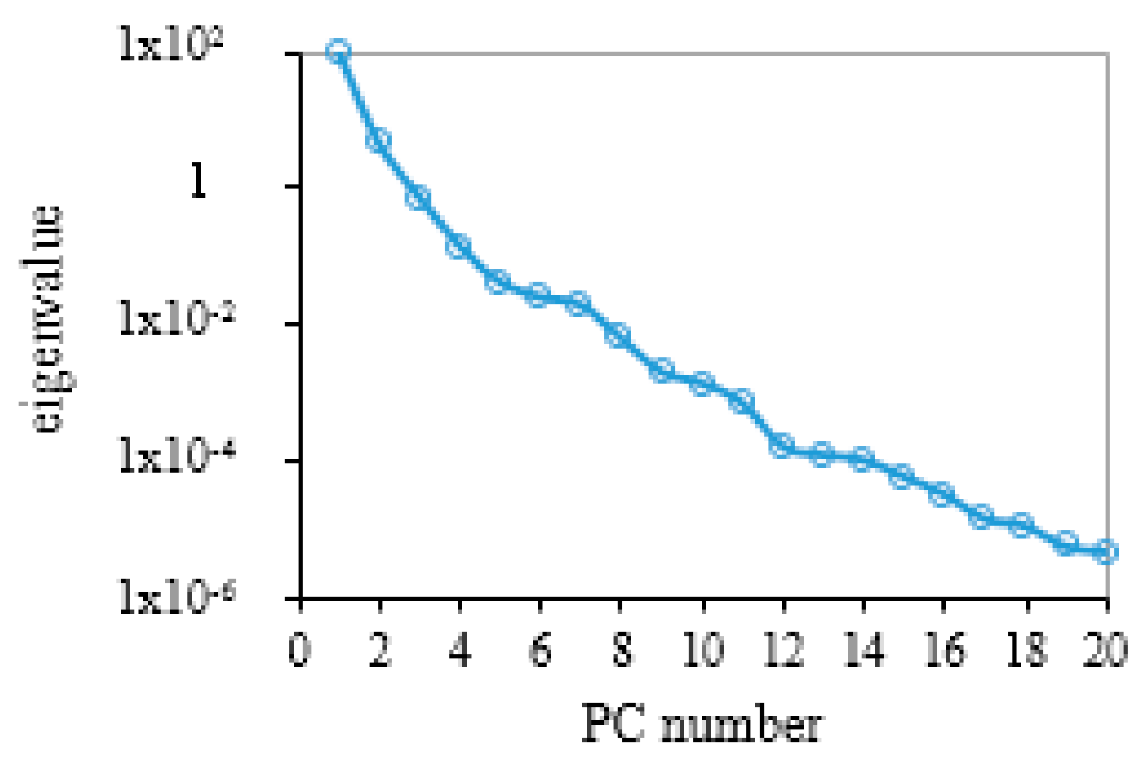
Figure 3.
The five leading principal components (PCs) derived from the simulated reflectance data for the ranges 400–2500 nm (a), 400–680 nm (b), 400–800 nm (c) and 900–2500 nm (d). PCi means the ith PC spectrum calculated from the simulated leaf reflectance dataset, which is also the eigenvector in the Equation (4).

Figure 4.
(a–j) Spectral root mean squared error (RMSE) between simulated leaf reflectance and reconstructed reflectance using the PCA method with different principal components (1-10PCs), (k) values of different principal components
Figure 4.
(a–j) Spectral root mean squared error (RMSE) between simulated leaf reflectance and reconstructed reflectance using the PCA method with different principal components (1-10PCs), (k) values of different principal components
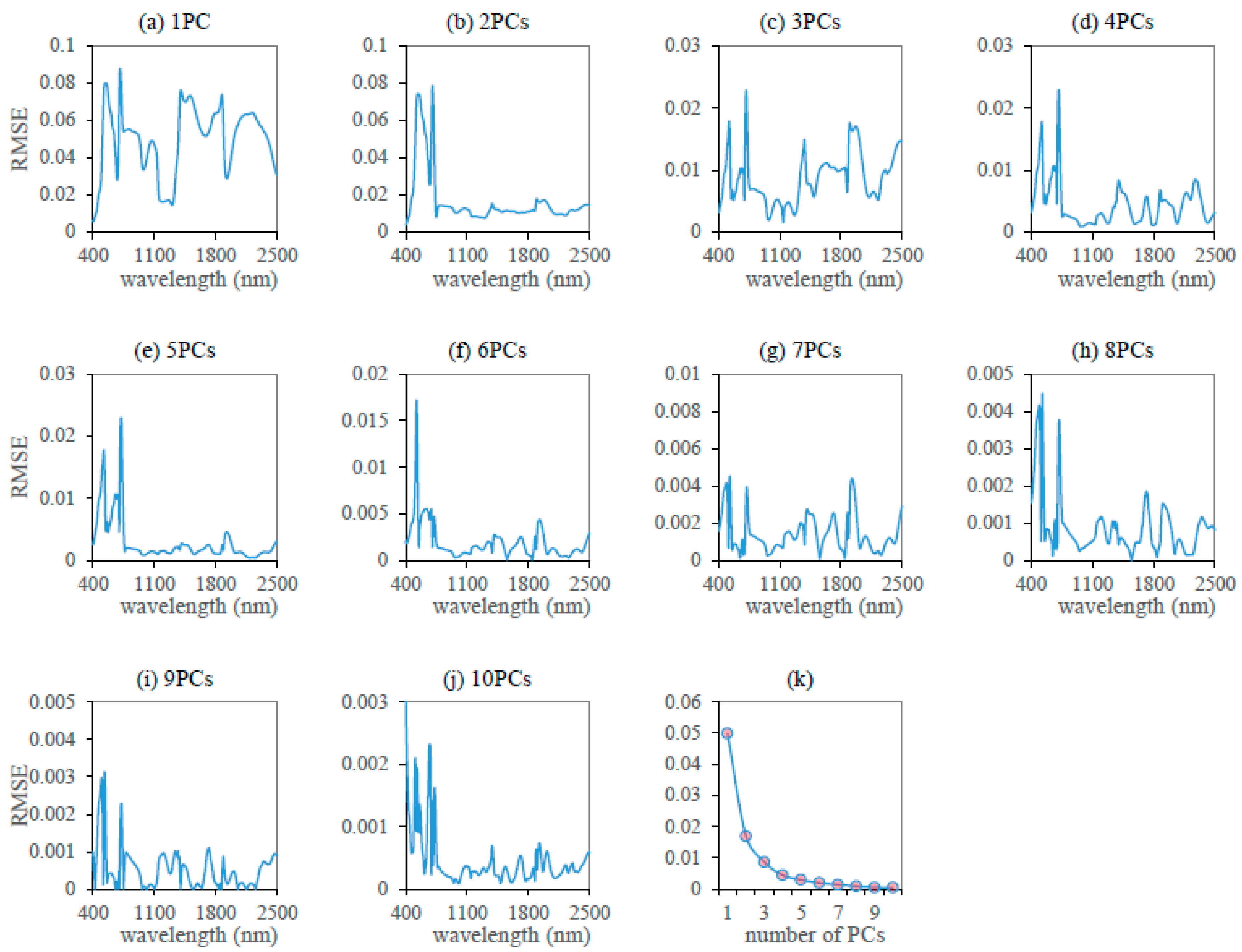
Figure 5.
Spectral root mean squared error (RMSE) between measured leaf reflectance and reconstructed reflectance using the ten leading principal components (PCs) for different spectral regions. X-1, X-2, X-3 and X-4 represent the spectral regions 400–2500 nm, 400–680 nm, 400–800 nm and 900–2500 nm. RMSE is root mean squared error.

Figure 6.
The regression models for the specific leaf weight (SLW) (a), equivalent water thickness (EWT) (b), chlorophyll content (c) and carotenoid content (d) derived using the weighting coefficients of the most sensitive principal component (PC), as given in Table 4. R2 is the determination coefficient.

Figure 7.
The results of the validation of the specific leaf weight (SLW) model based on the principal component analysis (PCA) method obtained using the simulated (a), ANGERS (b) and LOPEX’93 datasets (c). RMSE is the root mean squared error computed based on the SLW model as in Equation (6); R2 is the determination coefficient.

Figure 8.
The results of the validation of the equivalent water thickness (EWT) model based on the principal component analysis (PCA) method obtained using the simulated (a), ANGERS (b) and LOPEX’93 datasets (c). RMSE is the root mean squared error computed based on the EWT model as in Equation (7); R2 is the determination coefficient.
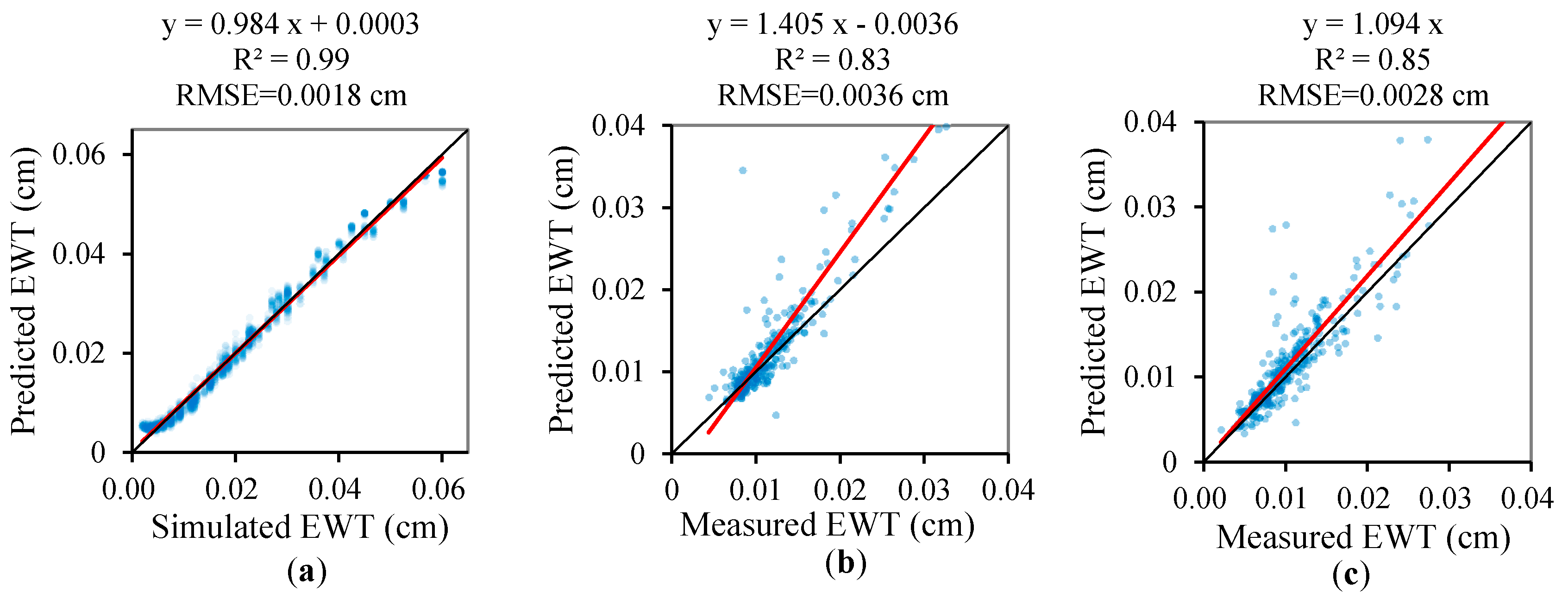
Figure 9.
The results of the validation of the statistical model of the chlorophyll content (Cab) based on the PCA data-driven method obtained using the simulated (a), ANGERS (b) and LOPEX’93 datasets (c). RMSE is the root mean squared error computed the Cab model as in Equation (8); R2 is the determination coefficient.
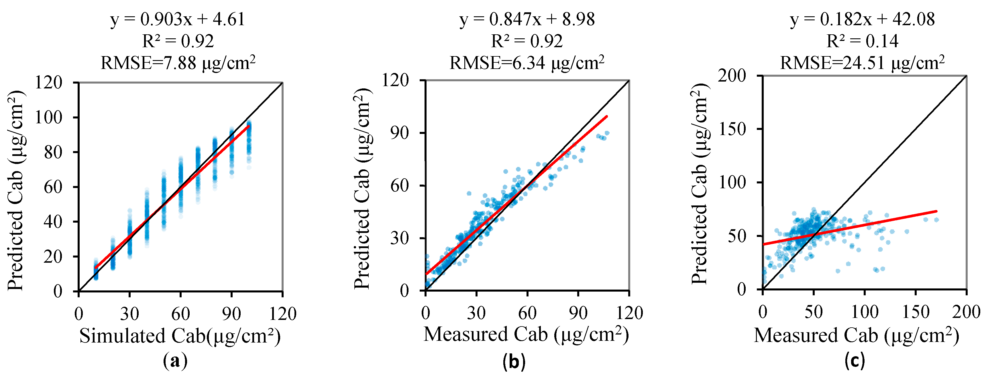
Figure 10.
The results of the validation of the statistical model of the carotenoid content based on the principal component analysis (PCA) method obtained using the simulated (a), ANGERS (b) and LOPEX’93 datasets (c). RMSE is the root mean squared error computed based on the Car model in Equation (9); R2 is the determination coefficient.


Table 1.
Inputs to the PROSPECT model used in the simulation experiment.
| Variable | Values | Unit | Description |
|---|---|---|---|
| Cab | 10–100 with an interval of 10 | μg/cm2 | Chlorophyll content |
| SLW | [0.002, 0.003, 0.004, 0.005, 0.0075, 0.01, 0.0125, 0.015, 0.0175, 0.02] | g/cm2 | Specific leaf weight |
| EWT | Derived from gravimetric water content (GWC %) and SLW GWC: 50–90% with an interval of 5% | cm | Equivalent water thickness |
| Car | [1/10, 1/8, 1/6, 1/5, 1/4, 1/3, 1/2] × Cab | μg/cm2 | Carotenoid content |
| N | Determined according to SLW | - | Leaf structure parameter |
Table 2.
Spectral indices employed for the estimation of leaf biochemical contents.
| Biochemical Component | Spectral Index | Formula | Reference |
|---|---|---|---|
| chlorophyll/Carotenoid | NDVI | NDVI = (R800 − R670)/(R800 + R670) | Rouse [76] |
| RVI | RVI = R800/R670 | Pearson and Miller [77] | |
| MTCI | MTCI = (R750 − R710)/(R710 − R680) | Dash and Curran [78] | |
| ND705 | (R750 − R705)/(R750 + R705) | Sims and Gamon [79] | |
| PRI | (R531 − R570)/(R531 + R570) | Gamon et al. [80] | |
| CIgreen | (RNIR/Rgreen) − 1 | Gitelson et al. [10] | |
| CIred edge | (RNIR/Rred edge) − 1 | Gitelson et al. [81] | |
| SIPI | (R800 − R445)/(R800 − R680) | Peñuelas et al. [82] | |
| Water | NDWI | NDWI = (R860 − R1240)/(R860 + R1240) | Gao [83] |
| WI | WI = R900/R970 | Peñuelas et al. [84] | |
| MSI | MSI = R1600/R820 | Hunt et al. [11] | |
| SLW | NDLMA | (R1368 − R1722)/(R1368 + R1722) | Féret et al. [85] |
| NDMI | (R1649 − R1722)/(R1649 + R1722) | Wang et al. [86] |
NDVI is the normalized difference vegetation index; RVI is the ratio vegetation index; MTCI is the MERIS terrestrial chlorophyll index; ND705 is the red-edge normalized difference vegetation index; PRI is the photochemical reflectance index; CIgreen is the green chlorophyll index; CIred edge is the red-edge chlorophyll index; SIPI is the structure-insensitive pigment index; NDWI is the normalized difference water index; WI is the water index; NDLMA is the normalized difference index for leaf mass per area (LMA); NDMI is the normalized dry matter index.
Table 3.
The spectral root mean squared error (RMSE) value of the reconstructed reflectance spectra derived using the ten leading principal components (PCs) for different spectral regions.
Table 3.
The spectral root mean squared error (RMSE) value of the reconstructed reflectance spectra derived using the ten leading principal components (PCs) for different spectral regions.
| Spectral Region (nm) | Training | Validation | ANGERS | LOPEX’93 | |
|---|---|---|---|---|---|
| 400–2500 | mean | 4.51 × 10⁻⁴ | 4.52 × 10⁻⁴ | 6.18 × 10⁻³ | 4.65 × 10⁻³ |
| maximum | 3.18 × 10⁻³ | 3.54 × 10⁻³ | 2.86 × 10⁻² | 1.87 × 10⁻² | |
| 400–680 | mean | 6.99 × 10⁻⁵ | 7.78 × 10⁻⁵ | 1.10 × 10⁻³ | 6.36 × 10⁻⁴ |
| maximum | 4.48 × 10⁻⁴ | 4.83 × 10⁻⁴ | 3.35 × 10⁻³ | 4.19 × 10⁻³ | |
| 400–800 | mean | 1.12 × 10⁻⁴ | 1.19 × 10⁻⁴ | 2.91 × 10⁻³ | 3.38 × 10⁻³ |
| maximum | 5.81 × 10⁻⁴ | 6.32 × 10⁻⁴ | 9.56 × 10⁻³ | 1.77 × 10⁻² | |
| 900–2500 | mean | 5.57 × 10⁻⁵ | 5.56 × 10⁻⁵ | 4.96 × 10⁻³ | 2.51 × 10⁻³ |
| maximum | 1.69 × 10⁻⁴ | 1.75 × 10⁻⁴ | 2.37 × 10⁻² | 8.99 × 10⁻³ | |
Table 4.
The coefficients of determination between the weighting coefficients of the principal components (PCs) and the leaf biochemical contents of the training dataset for the spectral regions 400–2500 nm (S1), 400–680 nm (S2), 400–800 nm (S3) and 900–2500 nm (S4).
Table 4.
The coefficients of determination between the weighting coefficients of the principal components (PCs) and the leaf biochemical contents of the training dataset for the spectral regions 400–2500 nm (S1), 400–680 nm (S2), 400–800 nm (S3) and 900–2500 nm (S4).
| Cab μg/cm2 | Car μg/cm2 | EWT cm | SLWg/cm2 | |||||||||||||
|---|---|---|---|---|---|---|---|---|---|---|---|---|---|---|---|---|
| S1 | S2 | S3 | S4 | S1 | S2 | S3 | S4 | S1 | S2 | S3 | S4 | S1 | S2 | S3 | S4 | |
| PC1 | 0.06 | 0.81 | 0.18 | 0.00 | 0.04 | 0.42 | 0.10 | 0.00 | 0.38 | 0.02 | 0.08 | 0.49 | 0.55 | 0.06 | 0.21 | 0.59 |
| PC2 | 0.14 | 0.67 | 0.83 | 0.00 | 0.06 | 0.29 | 0.40 | 0.00 | 0.69 | 0.01 | 0.01 | 0.94 | 0.38 | 0.04 | 0.03 | 0.40 |
| PC3 | 0.62 | 0.00 | 0.11 | 0.00 | 0.30 | 0.18 | 0.00 | 0.00 | 0.23 | 0.00 | 0.00 | 0.04 | 0.03 | 0.00 | 0.01 | 0.31 |
| PC4 | 0.11 | 0.16 | 0.02 | 0.00 | 0.05 | 0.09 | 0.18 | 0.00 | 0.14 | 0.00 | 0.00 | 0.14 | 0.01 | 0.01 | 0.00 | 0.07 |
| PC5 | 0.01 | 0.10 | 0.00 | 0.00 | 0.00 | 0.02 | 0.12 | 0.00 | 0.00 | 0.01 | 0.01 | 0.01 | 0.36 | 0.02 | 0.01 | 0.30 |
| PC6 | 0.06 | 0.01 | 0.00 | 0.00 | 0.00 | 0.00 | 0.12 | 0.00 | 0.01 | 0.00 | 0.01 | 0.00 | 0.00 | 0.01 | 0.02 | 0.01 |
| PC7 | 0.01 | 0.01 | 0.00 | 0.00 | 0.17 | 0.00 | 0.07 | 0.00 | 0.00 | 0.00 | 0.00 | 0.01 | 0.00 | 0.01 | 0.01 | 0.07 |
| PC8 | 0.00 | 0.01 | 0.00 | 0.00 | 0.01 | 0.00 | 0.06 | 0.00 | 0.03 | 0.00 | 0.04 | 0.01 | 0.01 | 0.00 | 0.11 | 0.02 |
| PC9 | 0.02 | 0.01 | 0.03 | 0.00 | 0.00 | 0.00 | 0.03 | 0.00 | 0.01 | 0.04 | 0.05 | 0.00 | 0.21 | 0.10 | 0.14 | 0.00 |
| PC10 | 0.00 | 0.00 | 0.01 | 0.00 | 0.06 | 0.00 | 0.00 | 0.00 | 0.00 | 0.00 | 0.10 | 0.00 | 0.02 | 0.00 | 0.22 | 0.00 |
S1, S2, S3, and S4 represent the spectral regions 400–2500 nm, 400–680 nm, 400–800 nm and 900–2500 nm. SLW, EWT, Cab and Car represent specific leaf weight, equivalent water thickness, chlorophyll content and carotenoid content, respectively. The bold font for numbers indicates the highest values.
Table 5.
The vegetation index (VI)-based models of leaf biochemical contents.
| Spectral Index | Regression Model | R2 |
|---|---|---|
| NDVI | (Cab) | 0.78 |
| (Car) | 0.51 | |
| RVI | (Cab) | 0.89 |
| (Car) | 0.59 | |
| MTCI | (Cab) | 0.90 |
| y = (Car) | 0.43 | |
| ND705 | (Cab) | 0.94 |
| y = (Car) | 0.61 | |
| PRI | (Cab) | 0.02 |
| y = (Car) | 0.21 | |
| SIPI | (Cab) | 0.72 |
| y = (Car) | 0.41 | |
| CIgreen | (Cab) | 0.91 |
| (Car) | 0.53 | |
| CIred edge | (Cab) | 0.89 |
| (Car) | 0.50 | |
| NDWI | y = 0.58x − 0.01 (EWT) | 0.95 |
| WI | y = 0.68x − 0.69 (EWT) | 0.95 |
| MSI | (EWT) | 0.97 |
| NDLMA | y = (SLW) | 0.83 |
| NDMI | y = (SLW) | 0.97 |
SLW, EWT, Cab and Car represent specific leaf weight, equivalent water thickness, chlorophyll content and carotenoid content, respectively. NDVI is the normalized difference vegetation index; RVI is the ratio vegetation index; MTCI is the MERIS terrestrial chlorophyll index; ND705 is the red-edge normalized difference vegetation index; PRI is the photochemical reflectance index; CIgreen is the green chlorophyll index; CIred edge is the red-edge chlorophyll index; SIPI is the structure-insensitive pigment index; NDWI is the normalized difference water index; WI is the water index; NDLMA is the normalized difference index for leaf mass per area (LMA); NDMI is the normalized dry matter index. R2 is the determination coefficient.
Table 6.
Results for the validation of the accuracy of the VI-based models of specific leaf weight (SLW) and equivalent water thickness (EWT).
Table 6.
Results for the validation of the accuracy of the VI-based models of specific leaf weight (SLW) and equivalent water thickness (EWT).
| Simulated | ANGERS | LOPEX’93 | |||
|---|---|---|---|---|---|
| SLW | NDLMA | R2 | 0.78 | 0.79 | 0.56 |
| RMSE | 0.0028 | 0.0018 | 0.0018 | ||
| NDMI | R2 | 0.95 | 0.73 | 0.7 | |
| RMSE | 0.0016 | 0.0025 | 0.0021 | ||
| PCA | R2 | 0.92 | 0.81 | 0.58 | |
| RMSE | 0.00169 | 0.00173 | 0.00178 | ||
| EWT | NDWI | R2 | 0.95 | 0.56 | 0.53 |
| RMSE | 0.0041 | 0.0044 | 0.0073 | ||
| WI | R2 | 0.96 | 0.75 | 0.61 | |
| RMSE | 0.0053 | 0.004 | 0.0094 | ||
| MSI | R2 | 0.96 | 0.77 | 0.83 | |
| RMSE | 0.0043 | 0.0037 | 0.0028 | ||
| PCA | R2 | 0.99 | 0.83 | 0.85 | |
| RMSE | 0.0018 | 0.0036 | 0.0028 | ||
PCA represents the results calculated using the principal analysis method. NDWI is the normalized difference water index; WI is the water index; NDLMA is the normalized difference index for specific leaf weight(SLW); NDMI is the normalized dry matter index. RMSE is the root mean square error; R2 is the determination coefficient. The bold font for numbers indicates the highest R2 values or the lowest RMSE values.
Table 7.
Results for the validation of the accuracy of the VI-based models of chlorophyll content (Cab) and carotenoid content (Car).
Table 7.
Results for the validation of the accuracy of the VI-based models of chlorophyll content (Cab) and carotenoid content (Car).
| Cab (µg/cm2) | Car (µg/cm2) | ||||||
|---|---|---|---|---|---|---|---|
| Simulated | ANGERS | LOPEX’93 | Simulated | ANGERS | LOPEX’93 | ||
| NDVI | R2 | 0.66 | 0.41 | 0.02 | 0.26 | 0.35 | 0.003 |
| RMSE | 17.74 | 18.02 | 27.9 | 9.42 | 4.09 | 6.67 | |
| RVI | R2 | 0.75 | 0.14 | 0.004 | 0.29 | 0.12 | 0.0001 |
| RMSE | 14.31 | 26.4 | 34.08 | 9.03 | 6.19 | 7.93 | |
| MTCI | R2 | 0.9 | 0.59 | 0.13 | 0.22 | 0.64 | 0.04 |
| RMSE | 8.89 | 18.23 | 27.59 | 10.05 | 3.41 | 6.37 | |
| ND705 | R2 | 0.89 | 0.95 | 0.12 | 0.38 | 0.84 | 0.07 |
| RMSE | 10.09 | 5.41 | 25.33 | 8.4 | 2.32 | 6.08 | |
| CIgerrn | R2 | 0.91 | 0.92 | 0.13 | 0.36 | 0.75 | 0.1 |
| RMSE | 8.59 | 7.7 | 24.92 | 8.66 | 3.3 | 6.51 | |
| CIred edge | R2 | 0.89 | 0.95 | 0.14 | 0.3 | 0.71 | 0.07 |
| RMSE | 9.42 | 6.23 | 25.05 | 9.23 | 3.11 | 6.07 | |
| PRI | R2 | 0.02 | 0.33 | 0.01 | 0.35 | 0.18 | 0.0003 |
| RMSE | 29.52 | 23.17 | 26.46 | 9.06 | 6.53 | 6.35 | |
| SIPI | R2 | 0.92 | 0.92 | 0.14 | 0.48 | 0.7 | 0.04 |
| RMSE | 7.91 | 7.39 | 24.52 | 7.77 | 4.63 | 7.34 | |
| PCA | R2 | 0.92 | 0.92 | 0.14 | 0.73 | 0.71 | 0.13 |
| RMSE | 7.88 | 6.34 | 24.51 | 5.96 | 2.77 | 5.76 | |
PCA represents the results calculated using the principal analysis method. NDVI is the normalized difference vegetation index; RVI is the ratio vegetation index; MTCI is the MERIS terrestrial chlorophyll index; ND705 is the red-edge normalized difference vegetation index; PRI is the photochemical reflectance index; CIgreen is the green chlorophyll index; CIred edge is the red-edge chlorophyll index; SIPI is the structure-insensitive pigment index; RMSE is the root mean square error; R2 is the determination coefficient. The bold font for numbers indicates the highest R2 values or the lowest RMSE values.
Table 8.
Comparison of estimates of leaf biochemical contents made using the principal component analysis (PCA) method and the P-5 method. (P-5 represents the PROSPECT-5 model inversion method used by Féret et al. [71]).
Table 8.
Comparison of estimates of leaf biochemical contents made using the principal component analysis (PCA) method and the P-5 method. (P-5 represents the PROSPECT-5 model inversion method used by Féret et al. [71]).
| Leaf Biochemistries | Method | ANGERS | LOPEX’93 |
|---|---|---|---|
| EWT cm | PCA | 0.0036 | 0.0028 |
| P-5 | 0.0020 | 0.0017 | |
| SLW g/cm2 | PCA | 0.00173 | 0.00178 |
| P-5 | 0.0026 | 0.0034 | |
| Cab µg/cm2 | PCA | 6.34 | 24.51 |
| P-5 | 5.17 | 32.35 | |
| Car µg/cm2 | PCA | 2.41 | 6.20 |
| P-5 | 2.77 | 5.76 |
SLW, EWT, Cab and Car represent specific leaf weight, equivalent water thickness, chlorophyll content and carotenoid content, respectively. The bold font for numbers indicates the lower RMSE values.
Table 9.
The statistical parameters of the validation results for the simulated, ANGERS and LOPEX’93 datasets.
Table 9.
The statistical parameters of the validation results for the simulated, ANGERS and LOPEX’93 datasets.
| Simulated Validation | ANGERS | LOPEX | |||||||||||||
|---|---|---|---|---|---|---|---|---|---|---|---|---|---|---|---|
| R² | RMSE | Bias | SL | INTC | R² | RMSE | Bias | SL | INTC | R² | RMSE | Bias | SL | INTC | |
| SLW | 0.92 | 0.00168 | −2.0% | 0.9 | 7 × 10⁻⁴ | 0.81 | 0.00173 | 29.8% | 0.656 | 2 × 10⁻⁴ | 0.58 | 0.00178 | 3.6% | 0.845 | 8 × 10⁻⁴ |
| EWT | 0.99 | 0.002 | −1.3% | 0.984 | 3 × 10⁻⁴ | 0.83 | 0.0036 | 9.7% | 1.40 | −0 | 0.85 | 0.0028 | 9.8% | 1.09 | 0 |
| Cab | 0.92 | 7.88 | −1.3% | 0.903 | 4.61 | 0.92 | 6.34 | 11.2% | 0.847 | 8.98 | 0.14 | 24.51 | 3.1% | 0.182 | 42.08 |
| Car | 0.73 | 5.96 | −7.6% | 0.54 | 5.00 | 0.71 | 2.77 | 1.9% | 0.759 | 2.24 | 0.13 | 5.76 | 11.6% | 0.2 | 9.93 |
R2 is the determination coefficient; RMSE is the root mean square error; Bias is the relative difference between the estimated value and the measured value; SL and INTC are slope and intercept.
© 2017 by the authors. Licensee MDPI, Basel, Switzerland. This article is an open access article distributed under the terms and conditions of the Creative Commons Attribution (CC BY) license (http://creativecommons.org/licenses/by/4.0/).
Share and Cite
MDPI and ACS Style
Liu, L.; Song, B.; Zhang, S.; Liu, X. A Novel Principal Component Analysis Method for the Reconstruction of Leaf Reflectance Spectra and Retrieval of Leaf Biochemical Contents. Remote Sens. 2017, 9, 1113. https://doi.org/10.3390/rs9111113
AMA Style
Liu L, Song B, Zhang S, Liu X. A Novel Principal Component Analysis Method for the Reconstruction of Leaf Reflectance Spectra and Retrieval of Leaf Biochemical Contents. Remote Sensing. 2017; 9(11):1113. https://doi.org/10.3390/rs9111113
Chicago/Turabian StyleLiu, Liangyun, Bowen Song, Su Zhang, and Xinjie Liu. 2017. "A Novel Principal Component Analysis Method for the Reconstruction of Leaf Reflectance Spectra and Retrieval of Leaf Biochemical Contents" Remote Sensing 9, no. 11: 1113. https://doi.org/10.3390/rs9111113
Note that from the first issue of 2016, this journal uses article numbers instead of page numbers. See further details here.