Comparison of Retrieved L2 Products from Four Successive Versions of L1B Spectra in the Thermal Infrared Band of TANSO-FTS over the Arctic Ocean

Abstract

This paper concentrates on the calibration/validation of the Thermal and Near Infrared Sensor for Carbon Observation (TANSO)–Fourier Transform Spectrometer (FTS) spectra in the thermal infrared (TIR) spectral region (B4 band) over the Arctic Ocean. We have performed inter-comparisons of the retrieved L2 products from four successive versions of L1B products (V150, V160, V201, V203) to check the differences and the improvement in the spectral and radiometric calibration of TANSO-FTS spectra in the narrow spectral domain of 940–980 cm⁻¹ covering CO₂ lines of the so-called laser band in the rather clear 10.4 μm atmospheric window, allowing sounding down to the lowest atmospheric layers. To our knowledge, this is the first attempt to retrieve XCO₂ from this spectral region. The period covered is the summer months (July, August, September) and the years from 2009 to 2015. Internal comparisons of L1B TANSO-FTS spectra, as well as comparisons of retrieved L2 products, i.e., T_surf (sea surface temperature or SST) and the retrieved column-averaged dry air volume mixing ratio XCO₂ derived with the same algorithm are presented. The overall trend in the CO₂ column-averaged VMR is well captured over the six year period for Green-house Gases Observing Satellite (GOSAT), but calibration issues are still hindering the use of TANSO-FTS TIR spectra for accurate and stable XCO₂ and T_surf products. However, an internal comparison of the successive L1B versions is possible and helpful to make progress with respect to the radiometric and spectral calibration TIR spectra collected by TANSO-FTS on GOSAT.

1. Introduction

Carbon dioxide (CO₂) in the atmosphere is well-known as the strongest greenhouse gas (see e.g., [1]), with concentrations measured with ground-based, airborne, and balloon-borne instruments, as well as concentrations derived from satellite sensors. Long-term observations have been performed from Mauna Loa, Hawaii, and from the South Pole starting in the late 1950s [2]. Since that period, worldwide comprehensive CO₂ observations in the atmosphere have been performed, including ground-based in situ or remote sensing data, tall towers, and aircraft flask sampling, as well as balloon-borne measurements, such as AirCore sampling systems [3]. Atmospheric CO₂ concentrations have gradually increased at a globally averaged annual rate of 2.2 ± 0.1 ppmv from 1998 to 2011, although their growth rate has a relatively large inter-annual variation [1]. Upper atmospheric CO₂ observations have been made in many areas by several projects using commercial airliners (e.g., [4]).

Atmospheric CO₂ observations by satellite sensors are usually based on CO₂ absorption band observations in the shortwave infrared (SWIR) regions around 1.6 and 2.0 μm. However, thermal infrared (TIR) regions between 15.5 and 12.5 μm, and around 4.3 μm, are also used [3]. As an example, the Scanning Imaging Absorption Spectrometer for Atmospheric Chartography (SCIAMACHY) on the Environmental Satellite (ENVISAT) observed CO₂ column-averaged dry-air mole fractions (XCO₂) from spectra at 1.57 μm [5]. The Thermal and Near Infrared Sensor for Carbon Observation (TANSO)–Fourier Transform Spectrometer (FTS) on board the Green-house Gases Observing Satellite (GOSAT), which was launched in 2009 [6] has observed XCO₂ with good precision using the 1.6 and/or 2.0 μm CO₂ absorption bands. The Orbiting Carbon Observatory 2 (OCO-2) was successfully launched in 2014, and started regular observations of XCO₂ with high spatial resolution [7]. Earlier satellite experiments allowed the inferring of CO₂ observations from TIR absorption bands: the High-Resolution Infrared Sounder (HIRS) [8], the Atmospheric Infrared Sounder (AIRS) [9], the Tropospheric Emission Spectrometer (TES) [10], and the Infrared Atmospheric Sounding Interferometer (IASI), which allowed the derivation of mid-atmospheric CO₂ amounts from their TIR spectra [11]. In addition to its NIR and SWIR bands [12], TANSO-FTS also has a TIR band that has been used in the present study. Numerous studies on the use of XCO₂ retrieved from satellite sensors for estimating sources and sinks (see e.g., [13] or [14]) have highlighted the importance of accuracy (no regional bias) that could hamper global inversions, particularly in regions where surface measurements are sparse, like in the Arctic. However, the use of mid-tropospheric CO₂ data (which is accessible from TIR soundings) in the inversion analysis of CO₂ surface fluxes is reducing the a posteriori flux errors, particularly in tropical Asian regions [15].

The present study focuses on the calibration and validation of TIR measurements from TANSO-FTS onboard the GOSAT satellite [16,17] over the Arctic Ocean, a very important region of the globe in which the effect of climate change can be detected over short time periods. The periods when GOSAT cannot make useful observations in the SWIR (sun too low, night, clouds), hamper the estimation of the global carbon budget. GOSAT measurements in band B4 (or thermal infrared = TIR) have not been used so far as thoroughly as those made in the SWIR. The potential of TIR should be studied in particular in the framework of the TIR/SWIR synergy [3] expected to provide more information on the vertical distribution of CO₂. In this respect, the current quality of TANSO-FTS TIR spectra and the precision of the XCO₂ retrievals have be analyzed in detail.

In this study, we used four different versions of the TIR spectra of TANSO-FTS to compare our retrieved L2 products using exactly the same homemade spectral inversion algorithm (called LARA, see Section 3) in order to estimate the impact of changes in the various versions of L1B products in B4 on the different retrieved L2 products. Our goal was to quantify the differences between versions and to contribute to the assessment of the quality of the new versions.

2. Instruments and Data

2.1. TANSO-FTS Instrument Onboard GOSAT.

GOSAT, in a sun-synchronous polar orbit around 666 km, has a revisit cycle of three days and an equator-crossing time of 13:00 LT. It covers almost the entire Earth from 85°N to 85°S [16]. The TANSO-FTS instrument has four bands in the range of 0.758–0.775 μm (Band 1 or B1), 1.56–1.72 μm (Band 2 or B2), and 1.92–2.08 μm (Band 3 or B3) in the SWIR region, and also 5.5–14.3 μm (Band 4 or B4) in the TIR region with a spectral sampling of about 0.2 cm⁻¹. The size of its instantaneous field of view or IFOV is 15.8 mrad, which corresponds at nadir to a circular footprint of approximately 10.5 km at the Earth’s surface. TANSO-FTS has several pointing patterns. The maximum off-nadir pointing angle is ±35° in the cross-track direction and ±20° in the along-track direction [16]. The spectral data of B4 Level 1B products recorded from 2009 to 2015 [17] and provided by JAXA were used for this study. The radiometric accuracy of this product is near 0.5 K in the range of 700–755 cm⁻¹ [4,18]. Observational patterns involved the five-point cross-track scan mode until July 2010, and the three-point cross-track scan mode after.

Table 1. Long-term operation status of TANSO-FTS.

Date	Configuration Changes	Nominal Pointing Pattern	Pointing System	Interferogram	Operation S = SWIR T = TIR
23 January 2009	Initial mode after launch	Five points	Primary	No bias	S + T
1 August 2010	Change of nominal pointing pattern	Three points	Primary	No bias	S + T
24 May 2014	Solar paddle/pointing system troubles	One and three point	Primary	800 fringe bias	S + T
26 January 2015	Change of pointing system	Three point	Secondary	800 fringe bias	S + T
2 August 2015	Cryo-cooler suspension	Three point	Secondary	650 fringe bias	S
14 September2015	Cryo-cooler restart	Three point	Secondary	1100 fringe bias	S + T

summarize the main operation changes during the last seven-year period [19].

Several incidents perturbed the production of L1B spectra in the thermal infrared band. The observations automatically stopped at 23:00 UT, 24 May 2014, due to a power generation shortage (half of the normal power) caused by a standstill of one of the two solar paddles failing to face the Sun, eventually to resume observation in the nadir mode at 23:00 UT, 30 May 2014, after prompt handling by JAXA. However, the available electric power was enough for nominal observations, ensuring continuation of nominal operations with one active paddle only and observations restarted on 2 July. Then a malfunction of the FTS pointing mechanism occurred, making the mirror too frequently unable to stand still after rotation to catch the next targeted IFOV within a normal time. However, switching to the redundant system was decided on 15 December 2014 and completed on 26 January 2015, enabling the continuation of steady observations.

Problems with the solar paddle and the TANSO-FTS pointing mechanism brought version changes in TIR L1B: versions processed and released (before/after) are V161.160/V161.161 for FTS L1B, and V02.21/V02.31 for FTS SWIR L2. There are no data released from 24 May, 20:28 UT to 30 May, 5:34 UT, 2014 due to the solar paddle disorder, and from 22:50 UT, 14 December 2014 to 23:59 UT, 31 January 2015 due to the pointing mechanism switching.

On 2 August 2015, TANSO-FTS TIR (B4) suspended its data processing due to a sudden shutdown of the cryo-cooler. The temperature of the TIR detector increased, while NIR and SWIR detectors (B1, B2, and B3) were operating normally. This anomaly on the cryo-cooler control electronics induced a shift in the zero path difference or ZPD position of the interferogram. The ZPD shift mechanism is sensitive to temperature and it was difficult to simulate the thermal distortion due to the cryo-cooler system failure. The new LlB V201 was able to correct the laser fringe-biased interferogram properly. On 14 September 2015, the cryo-cooler was restarted successfully. A new and stable ZPD position after the cooler restart was on the same side, but with a slightly larger bias than before 2 August. After 15 September, both SWIR and TIR have been acquired simultaneously with nominal three point, target, and glint modes.

2.2. TANSO-FTS L1B Spectra

Since the end of 2012, the French AERIS/ESPRI [20] infrastructure collects daily GOSAT data sets from the JAXA data center in order to sustain national scientific activity based on this data. Two main datasets are regularly recovered through the Connect/Direct protocol: TANSO-FTS (Fourier Transform Spectrometer) data from level 1B and level 2, and TANSO-CAI (Cloud and Aerosol Image) data from level 1B+ and 2.

All this data (currently more than 100 Tbytes) are stored on a dedicated machine and can be accessed on a cluster computer system of the IPSL data center [21]. For TANSO-FTS spectra (unapodized), a preliminary spectral calibration and resampling on a common sampling grid with a 0.200 cm⁻¹ spacing was performed.

Four different versions of the TANSO-FTS L1B spectra have been used in this study. The changes between these versions are the following:

• V15x.15x or V15x to simplify (V150.150 and V150.151) and V16x.16x of V16x to simplify (V160.160, V161.160, and V161.161): in these versions, the TIR radiometric calibration was optimized, the sampling interval non-uniformity correction was turned off, and gaps of the fringe count error and of the ZPD position error were corrected [22]
• V201.202 or V201 to simplify: sampling interval non-linearity correction for B1, B2, B3, and B4, modification of phase correction for B4, inclusion of the finite IFOV effect for B4 spectra, and modification of the ZPD bias correction algorithm [23]
• V203.203 or V203 to simplify: new TIR non-linearity correction applied [24].

The noise covariance matrix has been taken as a constant diagonal matrix (unapodised spectra). The value of the diagonal terms has been taken as the square of the noise equivalent delta radiance NEdR. The value of NEdR has been estimated as the mean, over all wavenumbers, of the standard deviation (over all the spectra used for retrieval) of the residual computed during a preliminary run of the retrievals.

In the region 940–980 cm⁻¹ used for our retrievals, this procedure yields a NEdR of 2.72 W/(cm² sr cm⁻¹). The corresponding noise equivalent delta temperature NEdT can then be derived from NEdR as NEdT = NEdR/(dB/dT(280 K)), where dB/dT is the derivative of the Planck function with respect to the temperature. At 960 cm^-1 this gives NEdR = 0.20 K.

3. Spectra Selection and Comparison Method

3.1. Radiative Transfer Model and Retrieval

The LATMOS (Laboratoire Atmosphère, Milieux, Observations Spatiales, France) Atmospheric Retrieval Algorithm (LARA), which has been developed over the years, is a homemade radiative transfer model associated with an inversion algorithm (see, e.g., [25,26,27]). The corresponding software has been used to analyze atmospheric spectra recorded using ground-based, balloon-, or satellite-borne experiments, both in absorption or emission mode, and for the limb or nadir geometry. LARA has been used to perform simulations of atmospheric spectra for the preparation of satellite experiments and for assessing the information content expected from instruments with different characteristics. The algorithm LARA allows the simultaneous inversion of spectra in several windows for the joint retrieval of vertical profiles (or slant column densities) of various species [25,26,27]. Surface temperature and emissivity, and if needed instrumental line shape or instrumental spectral shift may be fitted together with the concentrations of species. The LATMOS retrieval algorithm includes an accurate line-by-line radiative transfer model and an efficient minimization algorithm of the Levenberg-Marquardt type [28]. The full a posteriori error covariance matrix of the retrieved parameters is calculated within the retrieval process. The forward model (i.e., the radiative transfer model) uses molecular parameters that are extracted from the HITRAN 2012 database [29]. Individual line shapes are calculated with a Voigt profile which uses Lorentzian half-widths (with their temperature dependence exponent) and line shifts from HITRAN 2012. The calculation takes into account the water vapor continuum [30], as well as water vapor self-broadening. The reflected downward flux is taken into account using a single upward computation with a zenith angle of 55°, which was found to be nearly equivalent to a full angular integration. The reflected or diffused sunlight are modelled as well. For the present work, the algorithm was tailored to the specificities of the GOSAT spectra and geometry. The sea emissivity has been taken from Masuda [31], taking into account the zenith angle of the line of sight, while the surface temperature T_surf has been retrieved together with the relevant trace species amounts.

3.2. Configuration of the Inversion

We have performed retrievals from each individual spectrum (unapodized) of the different versions with our radiative transfer and retrieval code LARA, using as input the European Centre for Medium range Weather Forecast (ECMWF) ERA-Interim temperature and humidity profiles. As mentioned in Section 2, a preliminary spectral calibration and resampling on a common sampling grid with a 0.200 cm⁻¹ spacing was performed. We selected for the retrieval the spectral window (940–980 cm⁻¹), which contains the so-called CO₂ laser bands. To our knowledge, this is the first attempt to retrieve XCO₂ from this spectral region. The molecular species considered in the radiative transfer model were H₂O (water vapor), CO₂ (carbon dioxide), O₃ (ozone), CFC12 (dichlorodifluoromethane), and SF₆ (sulfur hexafluoride). For each spectrum, the following parameters have been retrieved:

• See surface temperature T_surf;
• One scaling factor for the initial profiles of CO₂ up to the tropopause, the stratospheric profile is kept constant and equal to the initial profile;
• Two scaling factors for the initial profiles of H₂O. One up to 800 m, a second between 900 m and the tropopause. In the stratosphere, the profile is taken to be constant and equal to the initial profile. In the layer between 800 m and 900 m, H₂O VMR is multiplied by a piecewise linear function of the altitude;
• One scaling factor for the initial profile of O₃;
• One spectral shift allowing to take into account small error in the spectral calibration; and
• One instrumental line shape parameter (optical path difference, see Section 4).

The initial profile of H₂O is taken from ECMWF ERA-Interim and interpolated at the exact time and location of the measurements. An implicit assumption here is that ECMWF ER-Interim temperature profiles (ERA-I) are accurate enough for the retrieval of T_surf and XCO₂. The initial profiles of CO₂ are taken in the troposphere as constant with a value equal to the yearly means of flask measurements performed at the Barrow station of the ESRL (NOAA) [32]. In the stratosphere, they are generated by the SAAP program of Geoffrey Toon [33]. For ozone, the subarctic summer profile of AFGL was used [34]. For CFC 12, we used constant profiles with values equal to the yearly mean of flask measurements performed at the Barrow station of the ESRL (NOAA) [32]. For SF₆ we used values retrieved from previous retrievals of ground-based and other satellite measurements (not described here). These values include the trend between 2009 and 2015.

From these retrieved state vector variables, the dry air column-averaged CO₂ volume mixing ratio (VMR) is derived together with corresponding quantities for H₂O and O₃ that should be considered here as “effective” parameters allowing to “fit” at best the observed spectra. The column-averaged dry air mixing ratio of carbon dioxide XCO₂ is then directly comparable to other measurements (the SWIR-derived quantity, for example). The amounts of water vapor and ozone do not have a direct geophysical meaning because the spectral interval chosen for T_surf and XCO₂ is far from optimized for water vapor and ozone retrievals. However, it is indeed necessary to include these two species in the state vector for getting a proper fit of the spectra and accurate (i.e., not biased) values of the target parameters T_surf and XCO₂.

Except for the shape of the a priori profiles, the retrieval is unconstrained and corresponds to a Levenberg-Marquardt (or least-squares) inversion rather than to the optimal estimation method (OEM) retrieval.

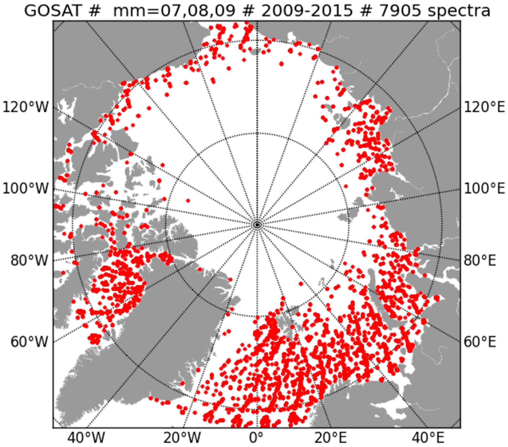
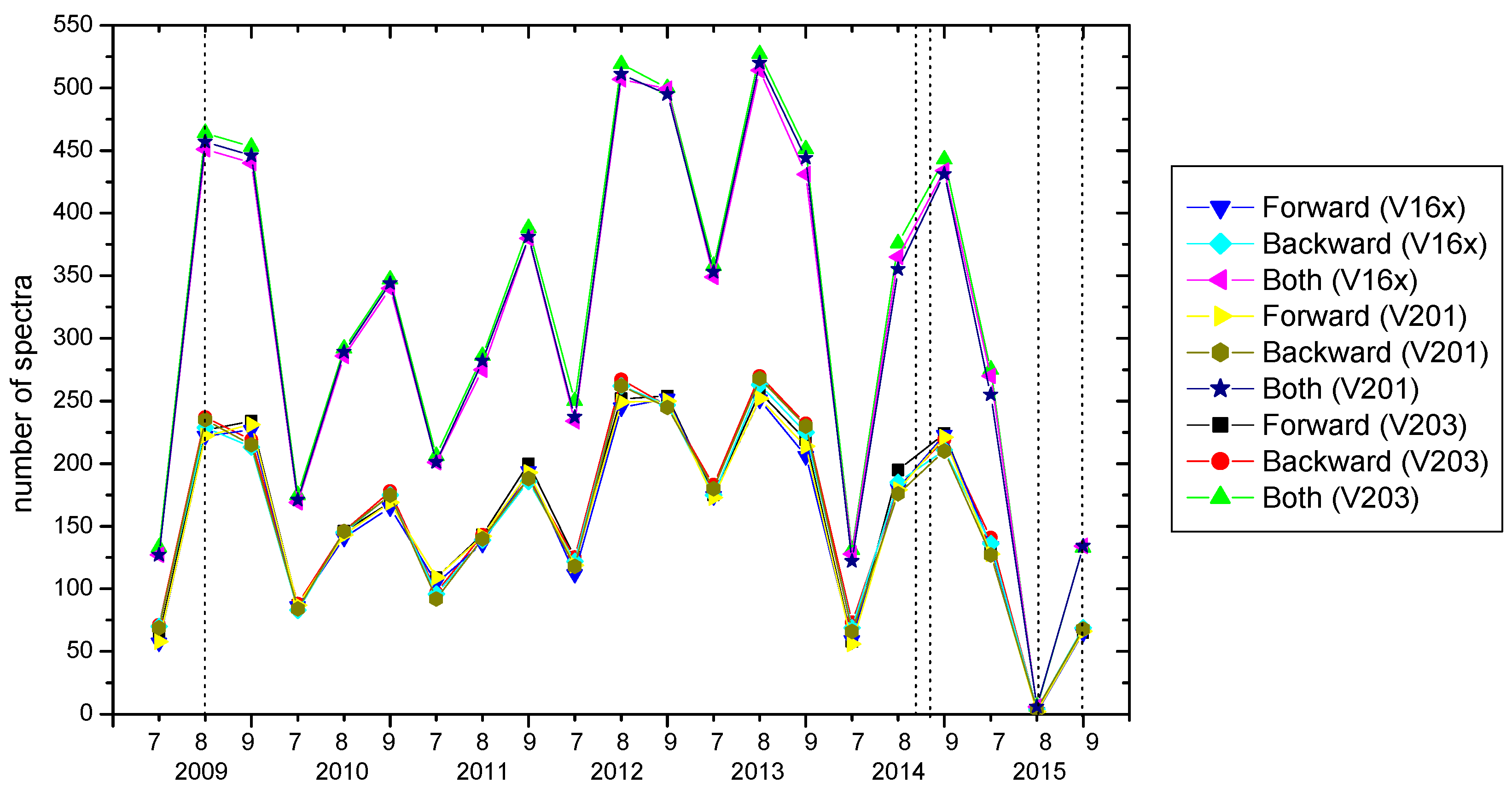
3.3. Selection of IFOVs

As mentioned in the introduction, the present study focused on TANSO-FTS measurements over the Arctic Ocean. This region was purposely chosen for comparison with nearly quasi-coincident soundings of IASIA and IASIB over ice-free footprints in the Arctic Ocean (see [35] for details). Only the summer months are considered, for which the sea surface in the selected satellite footprints is free of ice leading to spectra with signal to noise ratios high enough to allow for a significant retrieval of the target parameters.

A first step in the process is to select IFOVs/spectra of the TIR sounder in the latitude range [68°N–82°N] for the summer months July, August and September, i.e., mm = [07, 08, 09], and for a period covering the years between 2009 and 2015. We only kept IFOVs over the ocean (a sea/land flag is available for each TANSO-FTS measurement).

No special selection of day and night spectra was applied since we are in the TIR and since the period/region in which we are interested is mostly in daylight during the Arctic summer (but nighttime IFOVs are becoming more frequent in August and September depending on the latitude).

A first filtering is conducted for clear IFOVs. Since no cloud information was available for TANSO-FTS in the JAXA L1B products used in the present study, we have performed our own filtering for clear IFOVs using the spectrum itself (a variation of the split window technique). We could have used the TANSO-CAI browse images (as done manually/visually in a preliminary analysis) but the number of IFOVs to analyze was too high and it would have been unrealistic to do it systematically. In order to ensure that selected spectra are cloud/ice free, we compute the mean brightness temperature in three line-free micro-windows ([943.0531–943.4508 cm⁻¹], [960.1525–961.1467 cm⁻¹], [962.1408–962.7373 cm⁻¹]). A spectrum is considered as clear if the average over the three micro-windows of these mean temperature is greater than 274 K, and if their standard deviation is no more than 1 K (a high probability to avoid ice pack in the IFOV). At this stage the selected IFOVs are considered to be of type “clear, sea”.

The sensitivity of TIR sounders to the near-surface is largely driven by the thermal contrast, which is defined as the difference between the brightness temperature of the surface (including an emissivity value not strictly equal to unity) and the mean temperature of the air in the first discrete layer. Then, in order to ensure a reasonable sensibility to CO₂ close to the surface, we applied a second filter on the spectra (before the retrieval) using the line contrast in two regions of the TIR i.e., 820–930 cm⁻¹ (the so-called H₂O window) and 940–980 cm⁻¹ (the so-called CO₂ window). Observed line shapes (at the instrument resolution) can present parts in the emission due to a meteorological profile with temperature inversion not always well represented by the ECMWF model. In spectroscopic terms, the line contrast in the selected region is defined as the ratio of the root mean square (rms) of the brightness temperature spectrum below the continuum level (absorption contribution) to the rms above the continuum level (emission contribution). The continuum level (also called the scene temperature) is defined as a straight line between the two least absorbed micro-windows around 823 and 931 cm⁻¹ for the H₂O window and 943 and 962 cm⁻¹ for the CO₂ window. Based on this diagnostic, we eliminate the spectra for which the ratio of the depth of absorption lines over the depth of emission lines (accounting for the ringing of the unapodized TANSO-FTS spectra) is less than a threshold of 4.2 (for lines located between 820 and 940 cm⁻¹), and of 4.0 (for lines located between 940 and 980 cm⁻¹). With this technique, and the appropriate thresholding, IFOV/spectra prone to be inappropriate for accurate retrievals have been rejected. Only the IFOV/spectra of the “clear, sea, good line contrast” type are then ingested in the retrieval process. A third filter is applied on the T(z) and H₂O(z) profiles. We first eliminated all ECMWF ERA-I water vapor profiles reaching the saturation pressure. We selected then only IFOVs for which the ECMWF/ERA-I temperature profile (extracted and interpolated in time and space for any particular footprint) was appropriate. Over the Arctic Ocean, different geophysical situations can occur with respect to the temperature profile. We have distributed 25,218 ECMWF T(z) profiles into three classes: negative (normal) lapse rate profiles, noted T_a(z); quasi-isothermal profiles in the 0–1 km layer, noted T_b(z); and temperature inversion below 2 km, noted T_c(z). We found 7905 negative lapse rate profiles, 3089 isothermal profiles, and 18,951 profiles with temperature inversion. As an example, Figure 1 presents selected IFOVs for the 2009–2015 period. The profiles corresponding to the different categories are shown in Figure 2. The results of a sensitivity study (Figure 3) led us to retain only the negative lapse rate temperature profiles, i.e., of type T_a(z).

The sensitivity of the retrieved mean mixing ratio XCO₂ for different classes is shown in Figure 3. We define the sensitivity as the change in the retrieved ratio XCO₂ when the effective mixing ratio of a 1 km layer is increased by 1 ppmv. The simulations have been performed for a zero thermal contrast (meaning in an unfavorable situation) by choosing a surface temperature T_surf that verified B(T_surf) × ε = B(T₁) at the center of the retrieval spectral window (960 cm⁻¹). In this relation, T₁ is the temperature of the first atmospheric layer of the profile, ε the emissivity (taken from Masuda, with the zenith angle and wind speed equal to zero), and B is the Planck function. We have, in these conditions, a thermal contrast TC = 0.0 K, but for further checking of the influence of the thermal contrast between the surface and the first atmospheric layer, we have also computed the sensitivity function for TC = −2.0 K and TC = +2.0 K by changing T_surf correspondingly.

From Figure 3 one can clearly observe that the sensitivity to the 0–1 km layer is small in the normal lapse rate case, is near zero in the isothermal case, and becomes negative in the case of temperature inversion. Figure 3 also shows that for sounding the lowermost layer, TC = −2.0 K is less favorable than TC = 0.0 K, which is less favorable than TC = +2.0 K, whatever the class of the temperature profile. We can then conclude that T(z) must be of the normal (negative) lapse rate type for a reliable retrieval down to the surface. A selection is then particularly needed in this study because profiles that are isothermal in the lower layers or those presenting a temperature maximum near the top of the atmospheric marine boundary layer are quite frequent in summer over the Arctic Ocean [35].

Only the IFOV/spectra of the “clear, sea, normal lapse rate, good line contrast” type are then ingested in the retrieval process.

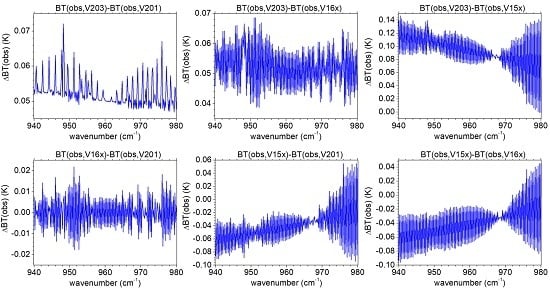
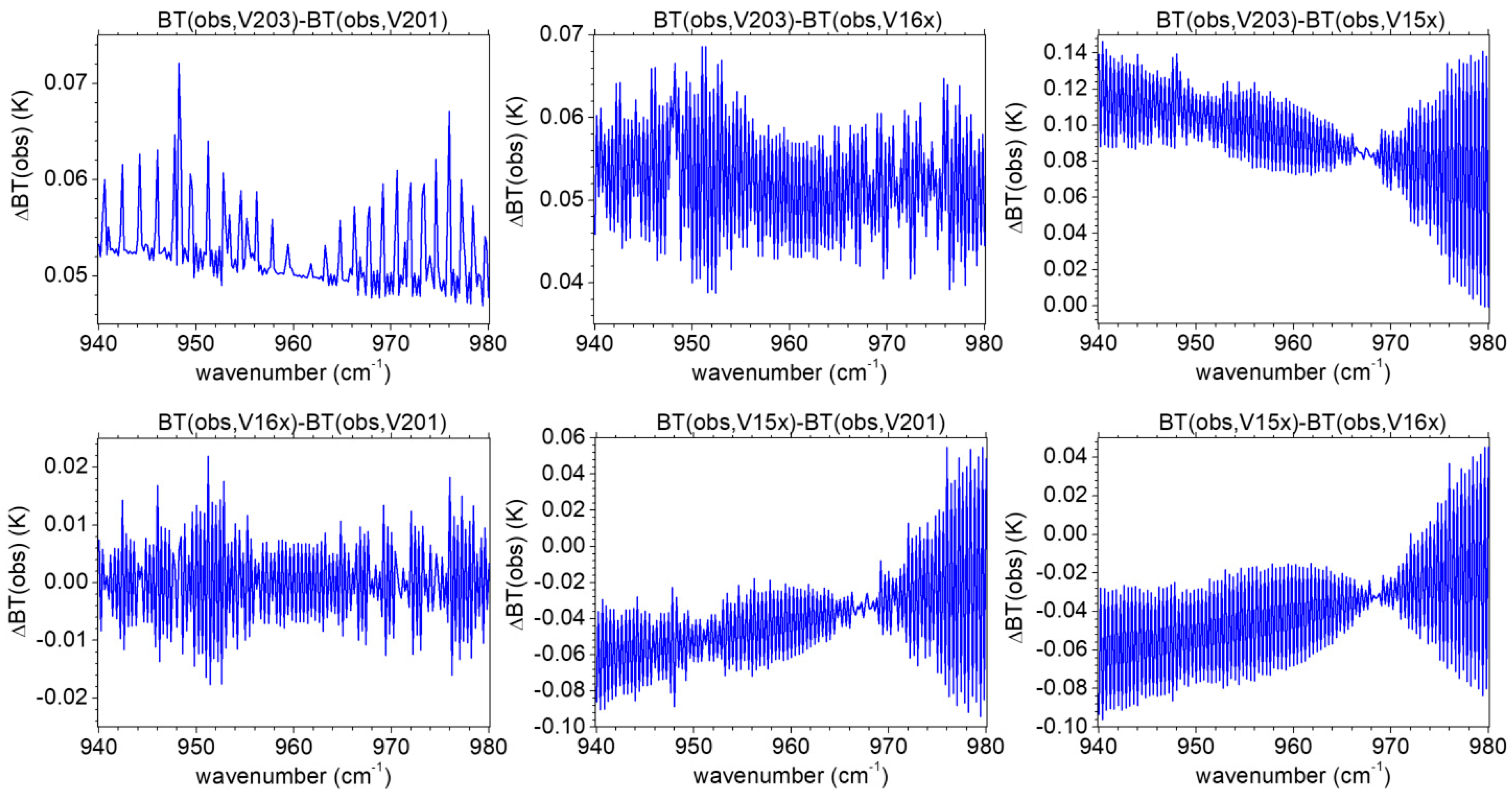
3.4. Differences between Versions at the L1B Level

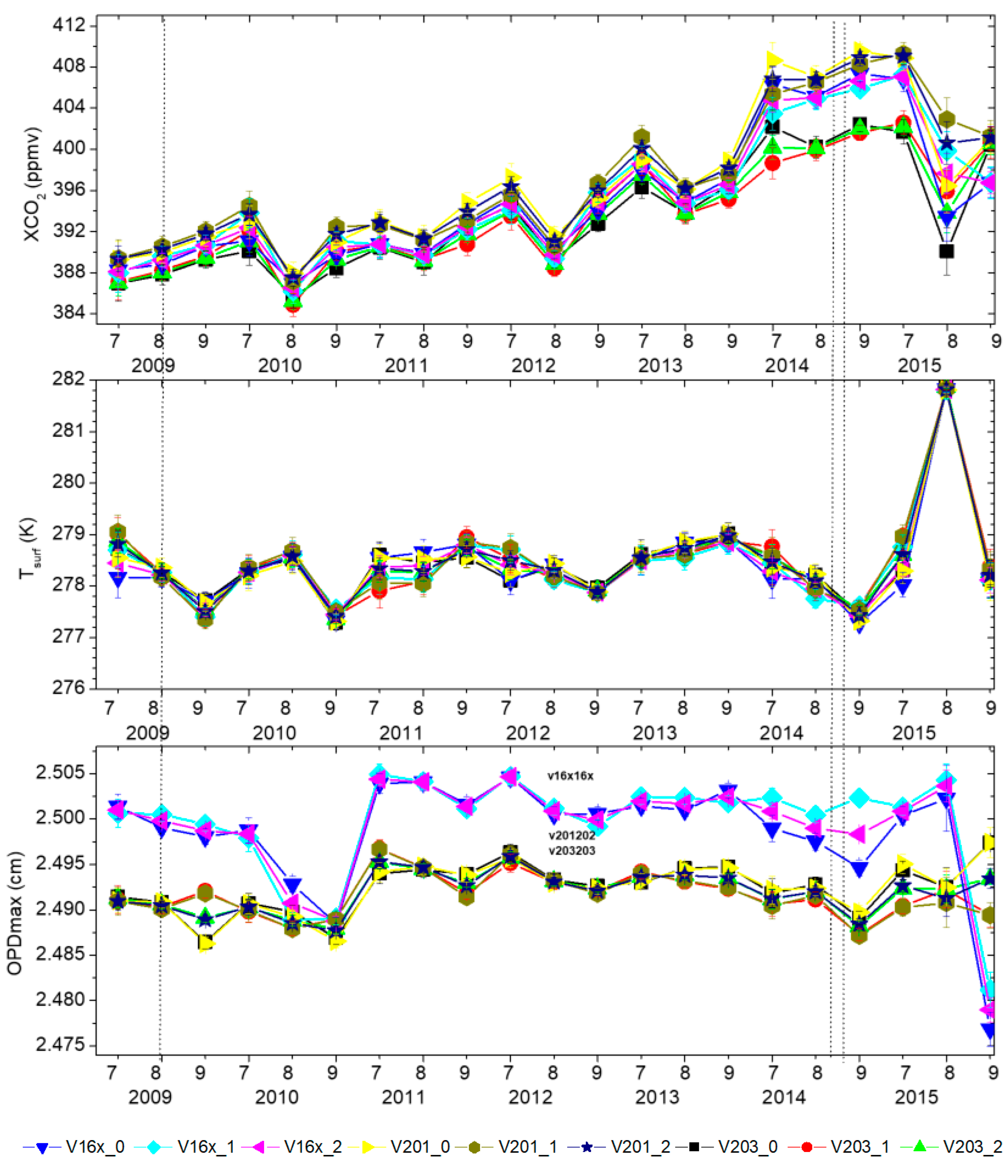
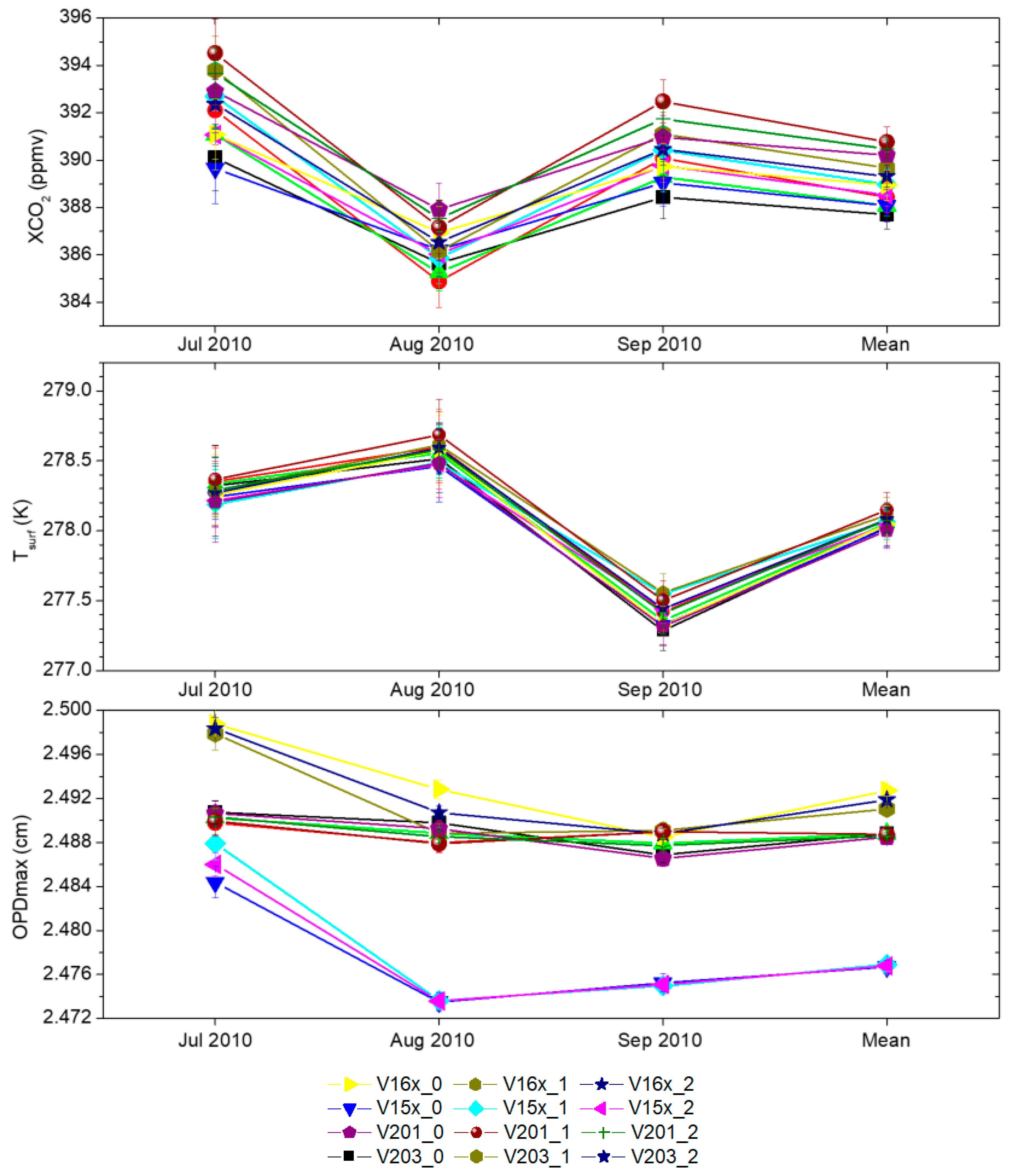
We computed the mean spectra for each version, and then the differences between these mean spectra. For the L1B comparisons we used spectra in brightness temperature for an easier comparison, but spectra in radiance units have been used for computing the mean spectra and as the input of the retrieval algorithm for generating L2 products (see the corresponding section). We recall that only the three summer months have been considered. For 2010, we selected spectra that were available for the four GOSAT FTS versions analyzed in this study (V15x, V16x, V201, and V203). For the other years and in the comparison of L2 products, we did not consider V15x spectra which were not available for all years. Figure 4 presents the brightness temperature differences (ΔBT) between the mean of L1B spectra BT(obs) computed from the four versions for 721 IFOVs for the months July, August, and September 2010. It was deemed useful in order to diagnose minute differences to combine the three months mm = [07, 08, 09] considered here (with, respectively, 151, 273, and 297 IFOVs) into the same set of 721 IFOVs. In Figure 4 (from the left to right and upper to lower panels) we can see that the BT of V201 are smaller than BT of V203 (ΔBT > 0). No oscillations are seen in the difference spectrum in which the major spectral signature (of H₂O and CO₂) are clearly visible. The differences are between 0.045 K and 0.075 K. The BT values of V16x are also smaller than the BT of V203 (ΔBT > 0) and are between 0.035 K and 0.070 K. We can see oscillations in the mean spectrum differences probably indicating a difference in the processing of interferograms to spectra. The same is true for the comparison of V15x with respect to V203: systematic oscillations are present, but the differences are larger and range from 0.00 K to 0.15 K. There is no systematic brightness temperature difference between V16x and V201, but we can notice oscillations in the ±0.025 K range. The differences between V15x and V201, as well as between V15x and V16x do present similar symptoms, i.e., oscillations and ΔBT values between −0.10 K and +0.05 K. Clearly, the differences between versions are related to some of the changes in the processing configuration introduced in Table 1, and they will impact the retrieved L2 products.

4. Results

We then explored the impact of these differences in L1B versions on the inversion of geophysical parameters. A large number of retrievals have been performed in exactly the same inversion configuration making the comparison of L2 TIR products feasible from four different versions of the TANSO-FTS spectra. This large set of results for “clear, sea, normal lapse rate, good line contrast” retrievals is useful for interesting analyses from the geophysical point of view. The full period 2009–2015 is available for checking the successive versions of L1B products from JAXA, even if the L1B spectra from version V15x have been kept at AERIS/ESPRI only for 2010 (hence the smaller number of spectra for this particular version) expecting that version V16x was superseding the older one. Then, for 2010, we selected spectra that were available for the four GOSAT FTS versions considered in this study (V15x, V16x, V201, and V203). For the other years, we did not consider V15x spectra that were not available.

The results of the retrievals are presented in this section. In the different figures, we present in sequence the time series of TIR retrievals (XCO₂ and T_surf) for version V203 that was initially assumed by us to be the best, and for versions V201, V16x, and V15x. Since this last version was considered as obsolete once V16x has been available, only a few files for V15x were preserved in the AERIS archive (only three months in summer 2010). This is why we will present results for the V15x version for July, August, and September 2010 separately.

Our retrievals have shown that the changes in the TANSO-FTS instrumental line shape (ILS) could have affected retrieved parameters. This is why we have performed a retrieval of the empirical FTS maximum optical path difference (OPD_max). In addition, because the sign of the OPD scan velocity could possibly change the ILS, we have considered separately the spectra recorded in the forward (F) or in the backward (B) direction of the scan mechanism (as well as the combination of the two). We present, hereafter, time series for the empirically-retrieved OPD_max. A major impact on the L1B TANSO-FTS spectra has been the cooler failure in August 2015.

In the following, time series of the retrieved parameters are plotted with a time scale referenced as a number; 1–3 for July, August, and September 2009; 4–6 for July, August, and September 2010; …19–21 for July, August, and September 2015. To illustrate the statistics, Figure 5 presents the time series of the population (number) of selected spectra differentiating the direction of the FTS moving mirror (forward=0, backward=1, both directions=2), and for three different TANSO-FTS L1B spectra versions (V15x, V16x, V201, V203). In the figures, we have used the notation already introduced to identify the corresponding L1B versions: V15x, V16x, V201, and V203. As mentioned in Section 2, a major impact on the L1B TANSO-FTS spectra has been the cooler failure in August 2015. This is why we plotted our retrieved time series, with and without August 2015 data.

On the graph in Figure 6 and Figure 7, plotted error bars are empirical uncertainties (1σ) estimated by the corresponding standard deviation (which are higher than theoretical uncertainties calculated in the retrieval process as described in inverse theory [36]). A first observation of the results for the retrieved maximum optical path difference shows that OPD_max is significantly different for the V16x data set, with OPD_max(V16x) > OPD_max(V15x, V201, or V203). This is not true for August 2015, for which, even if there are few IFOVs/spectra (index 8/2015 on the three panels in Figure 6), the mean values are not unexpected. However, the retrieved values are significantly lower for OPD_max(V16x) compared to the three other L1B versions’ retrievals. This is why we presented plots (with and without the two last monthly samples) allowing to obtain a better view of the time series.

Except for 2015, we can observe the main behavior for each version: OPD_max(July) > OPD_max(August) > OPD_max(September). The variation is less regular for 2013. A significant increase of OPD can be seen (for the four versions) between 2010 and 2011, whereas retrieved values are close to each other for September 2010, which is quite surprising.

In Figure 6, we can see that, except for 2009, XCO₂ has a minimum in August, and is increasing from 2009 to 2015, which is consistent with previous observations (see, e.g., [1]). T_surf has a maximum in August, except for 2009, and a minimum in September. No global trend can be observed for T_surf from 2009 to 2015 due to the inter-annual variability of the SST in the Arctic.

In Figure 7, we show, successively, for the months of July, August and September 2010, the retrieved XCO₂, the retrieved T_surf, the retrieved OPD_max (included as a parameter of the state vector in the present study), and the mean for the three months is also shown. For these three months the statistics for the four L1B version are, respectively, 774 spectra (V15x), 795 (V16x), 804 (V201), and 814 (V203).

5. Discussion

The analysis presented in Section 3.4 has shown that brightness temperature differences of 0.1 K can exist between various TANSO-FTS versions at the L1B level. In addition, two of the earlier versions (V15x and V16x) do present artefacts (oscillations) making them problematic for generating reliable retrieved products at the L2 level. Versions V201 and V203 are then probably more appropriate for discussing the geophysical products T_surf and XCO₂ derived using the LARA radiative transfer and spectral inversion package. Two major outcomes of our study can be summarized as follows: (i) The inter-annual variability of the sea surface temperature (T_surf or SST) for the ice free Arctic Ocean in the three summer months are significant and do not show a clear trend for the six-year span between 2009 and 2015. However, the SST maximum in August is clearly seen for all years (except 2009), with a significant cooling in September. (ii) The trend in XCO₂ at the regional scale of the Arctic for the six-year time span covered in the present study is clearly observed and is consistent with the global trend documented by ground based networks of more than 2 ppmv/year. Two difficulties arise in the TANSO-FTS data analysis, however. The year 2015 is clearly perturbed by the failure of the cryo-cooler and this specific year is considered as unreliable for a trend analysis. The differences (see the upper panel of Figure 6 for XCO₂) for 2014 between V201 and V203 (this last version having been provided by JAXA to external calibration/validation scientists) are significant. Assuming that V203 is the most reliable version an (interim) estimated trend of 2.6 ± 0.3 ppmv/year from July 2009 to July 2014 over the Arctic Ocean is obtained.

As mentioned previously, SF₆ has been taken into account in the forward model. Indeed, we observed a bias of about +2 ppmv on the retrieved XCO₂ when SF₆ in not introduced in the radiative transfer calculation. The XCO₂ standard deviations are also higher when determined without SF₆ in the calculations. In addition, differences between observed and calculated spectra (estimated χ²) are higher when SF₆ is not considered. The rather high spectral resolution of TANSO-FTS compared to other TIR sounders (e.g., IASI or AIRS) could explain the need to take into account sulfur hexafluoride. However, χ² (e.g., the quality of the fit of a given TANSO-FTS spectrum) presents no significant differences if SF₆ is fixed, or if it is retrieved. Furthermore, the retrieved T_surf standard deviation is lower when SF₆ is fixed than when it is retrieved. This is why SF₆ has been fixed in our retrievals with a different value for each year in order to account for the SF₆ trend.

We have performed studies (not reported here) of the impact of the uncertainty in the knowledge of T(z) from ERA-I using the OEM (optimum method formalism) of Rodgers [36] and the corresponding S_b covariance matrix (combined T and H₂O matrix) derived from the actual set of ERA-I profiles on an annual and monthly climatology for the summer months, i.e., July/August/September of the 2009–2015 period. In a similar manner as the effect on the retrieved target parameters of the assumed vertical temperature profile, the effect of the shape of the humidity profile could also have an impact. Thus a retrieval of the scaling factor of the humidity profile, as well as of the ozone profile have been performed within the LARA algorithm leading to the effective parameters XH₂O and XO₃ (the corresponding scaling factors are included in the state vector x). In particular, it proved to be very important to adjust the humidity in the lowest atmospheric layers to the spectra fit properly in the small interval 947.8–948.6 cm⁻¹ where a strong H₂O line is interfering with a CO₂ line and with the Q branch of the trace species SF₆ (also needed to match properly the spectral features in this particular micro-window). However, the full interval 940–980 cm⁻¹ was considered in the observation vector y.

6. Conclusions

The study presented in this paper was initiated to compare the capabilities of retrievals of T_surf and XCO₂ from GOSAT in one “surface window” i.e., the spectral region of 940–960 cm⁻¹ (~10.4 μm) for obtaining yearly time series (including variations within the summer months) and hopefully for producing climate quality records, at a regional scale in the summer over the Arctic Ocean for a period of six years. Another motivation was to compare with IASI-A (2010 to 2015) and IASI-B (2013 to 2015) in the latitude region [68°N, 80°N] (see [35]). From our study, we estimate that, for a single spectrum, the precision (not accuracy!) of the retrieved T_surf from GOSAT is ~0.05 K (1σ) for clear IFOVs, over sea in summer and with a normal atmospheric lapse rate T(z) profile (from ECMWF), but this statistical uncertainty (from the retrieval algorithm) does not include systematic errors. Our results show a significant variation of T_surf with latitude and between July/August/September, although the inter-annual variability does not show a trend in T_surf at the regional scale for the period covered.

For a single spectrum, we estimate that the precision (not accuracy!) of the retrieved XCO₂ from GOSAT in the TIR is ~6 ppmv (1σ) for clear IFOVs for the period, location, and season of this study (again without considering systematic radiometric errors). We recall that in our retrievals there is no a priori constraint on the XCO₂ value, except on the shape of the vertical distribution considered as the constant mixing ratio profile xCO₂ (z). The overall trend in the CO₂ column-averaged VMR is well captured over the six year period for GOSAT.

However, radiometric calibration issues (related to non-linearity correction, blackbody emissivity, and in-orbit changes in the FTS temperature) are presently under consideration by JAXA. They are still hindering the use of TANSO-FTS TIR spectra for accurate and stable XCO₂ and T_surf products. Indeed, it is very important to confirm the absolute radiometric calibration of TANSO-FTS in the TIR for providing a series of “climate quality variables” for T_surf, and possibly CO₂ in the not-so-well-documented Arctic Ocean region where the SWIR/NIR bands are not providing useful measurements. Other TIR sounders, especially IASI, will be a good reference for checking the new version of TANSO-FTS spectra in the TIR region (B4). The very stable IASI archive could help in this respect through quasi-coincidences in space and time occurring over the Arctic Ocean, a good target in ice-free conditions for checking the absolute radiometric calibration of TANSO-FTS in B4 with respect to IASI, considered by GSICS (WMO Global Space-based Inter-Calibration System, [37]) as a reference in infrared sounding. It is hoped that the expected new non-linearity correction of TANSO-FTS spectra in the TIR will reduce the observed differences. Indeed, a better radiometric calibration of the TIR spectra of TANSO-FTS should be implemented soon by JAXA. A detailed comparison of GOSAT and IASI T_surf from coinciding measurements of the two instruments over the Arctic region is under study, and we plan to publish the corresponding results next year.

As shown in this paper, the impact of instrumental line shape changes in TANSO-FTS has to be carefully examined. Since the launch of GOSAT (more than eight years) a very valuable archive of L0 TANSO-FTS TIR data has been acquired and could be very beneficial to the greenhouse gases and atmospheric composition communities provided a reliable re-processing is performed using the latest information on the identified problems and their subsequent correction. Major changes in the GOSAT platform and TANSO-FTS configurations have hindered a fully homogenized set of TIR spectra. New efforts towards a consistent and stable radiometric calibration of TANSO-FTS TIR spectra would be a very important asset for a successful GOSAT-2 mission.

References

1. Rajendra, K.P.; Myles, R.A.; Vicente, R.B.; John, B.; Wolfgang, C.; Renate, C.; John, A.C.; Leon, C.; Qin, D.; Purnamita, D.; et al. Climate Change 2014: Synthesis Report. Contribution of Working Groups I, II and III to the Fifth Assessment Report of the Intergovernmental Panel on Climate Change; IPCC: Geneva, Switzerland, 2014. [Google Scholar]
2. Keeling, C.D.; Chin, J.F.S.; Whorf, T.P. Increased activity of northern vegetation inferred from atmospheric CO2 measurements. Nature 1996, 382, 146–149. [Google Scholar] [CrossRef]
3. Saitoh, N.; Imasu, R.; Ota, Y.; Niwa, Y. CO2 retrieval algorithm for the thermal infrared spectra of the Greenhouse Gases Observing Satellite: Potential of retrieving CO2 vertical profile from high-resolution FTS sensor. J. Geophys. Res. 2009, 114, D17305. [Google Scholar] [CrossRef]
4. Machida, T.; Matsueda, H.; Sawa, Y.; Nakagawa, Y.; Hirotani, K.; Kondo, N.; Goto, K.; Nakazawa, T.; Ishikawa, K.; Ogawa, T. Worldwide Measurements of Atmospheric CO2 and Other Trace Gas Species Using Commercial Airlines. J. Atmos. Ocean. Technol. 2008, 25, 1744–1754. [Google Scholar] [CrossRef]
5. Buchwitz, M.; de Beek, R.; Burrows, J.P.; Bovensmann, H.; Warneke, T.; Notholt, J.; Meirink, J.F.; Goede, A.P.H.; Bergamaschi, P.; Körner, S.; et al. Atmospheric methane and carbon dioxide from SCIAMACHY satellite data: Initial comparison with chemistry and transport models. Atmos. Chem. Phys. 2005, 5, 941–962. [Google Scholar] [CrossRef]
6. Yokota, T.; Yoshida, Y.; Eguchi, N.; Ota, Y.; Tanaka, T.; Watanabe, H.; Maksyutov, S. Global concentrations of CO2 and CH4 retrieved from GOSAT: First preliminary results. Sola 2009, 5, 160–163. [Google Scholar] [CrossRef]
7. Crisp, D.; Pollock, H.R.; Rosenberg, R.; Chapsky, L.; Lee, R.A.M.; Oyafuso, F.A.; Frankenberg, C.; O’Dell, C.W.; Bruegge, C.J.; Doran, G.B.; et al. The on-orbit performance of the Orbiting Carbon Observatory-2 (OCO-2) instrument and its radiometrically calibrated products. Atmos. Meas. Tech. 2017, 10, 59–81. [Google Scholar] [CrossRef]
8. Chédin, A.; Serrar, S.; Scott, N.A.; Crevoisier, C.; Armante, R. First global measurement of mid tropospheric CO2 from NOAA polar satellites: Tropical zone. J. Geophys. Res. 2003, 108, 4581. [Google Scholar] [CrossRef]
9. Maddy, E.S.; Barnet, C.D.; Goldberg, M.; Sweeney, C.; Liu, X. CO2 retrievals from the Atmospheric Infrared Sounder: Methodology and validation. J. Geophys. Res. 2008, 113, D11301. [Google Scholar] [CrossRef]
10. Kulawik, S.S.; Jones, D.B.A.; Nassar, R.; Irion, F.W.; Worden, J.R.; Bowman, K.W.; Machida, T.; Matsueda, H.; Sawa, Y.; Biraud, S.C.; et al. Characterization of Tropospheric Emission Spectrometer (TES) CO2 for carbon cycle science. Atmos. Chem. Phys. 2010, 10, 5601–5623. [Google Scholar] [CrossRef]
11. Crevoisier, C.; Chédin, A.; Matsueda, H.; Machida, T.; Armante, R.; Scott, N.A. First year of upper tropospheric integrated content of CO2 from IASI hyperspectral infrared observations. Atmos. Chem. Phys. 2009, 9, 4797–4810. [Google Scholar] [CrossRef]
12. Saitoh, N.; Kimoto, S.; Sugimura, R.; Imasu, R.; Kawakami, S.; Shiomi, K.; Kuze, A.; Machida, T.; Sawa, Y.; Matsueda, H. Validation of GOSAT/TANSO-FTS TIR UTLS CO2 data (Version 1.0) using CONTRAIL measurements. Atmos. Meas. Tech. Discuss. 2015, 8, 12993–13037. [Google Scholar] [CrossRef]
13. Rayner, P.J.; O’Brien, D.M. The utility of remotely sensed CO2 concentration data in surface source inversions. Geophys. Res. Lett. 2001, 28, 175–178. [Google Scholar] [CrossRef]
14. Park, B.C.; Prather, M.J. CO2 source inversions using satellite observations of the upper troposphere. Geophys. Res. Lett. 2001, 28, 4571–4574. [Google Scholar] [CrossRef]
15. Niwa, Y.; Machida, T.; Sawa, Y.; Matsueda, H.; Schuck, T.J.; Brenninkmeijer, C.A.M.; Imasu, R.; Satoh, M. Imposing strong constraints on tropical terrestrial CO2 fluxes using passenger aircraft based measurements. J. Geophys. Res. 2012, 117, D11303. [Google Scholar] [CrossRef]
16. Kuze, A.; Suto, H.; Nakajima, M.; Hamazaki, T. Thermal and near infrared sensor for carbon observation Fourier-transform spectrometer on the Greenhouse Gases Observing Satellite for greenhouse gases monitoring. Appl. Opt. 2009, 48, 6716–6733. [Google Scholar] [CrossRef] [PubMed]
17. Kuze, A.; Suto, H.; Shiomi, K.; Urabe, T.; Nakajima, M.; Yoshida, J.; Kawashima, T.; Yamamoto, Y.; Kataoka, F.; Buijs, H. Level 1 algorithms for TANSO on GOSAT: Processing and on-orbit calibrations. Atmos. Meas. Tech. 2012, 5, 2447–2467. [Google Scholar] [CrossRef] [Green Version]
18. Kataoka, F.; Knuteson, R.O.; Kuze, A.; Suto, H.; Shiomi, K.; Harada, M.; Garms, E.M.; Roman, J.A.; Tobin, D.C.; Taylor, J.K.; et al. TIR Spectral Radiance Calibration of the GOSAT Satellite Borne TANSO-FTS With the Aircraft-Based S-HIS and the Ground-Based S-AERI at the Railroad Valley Desert Playa. IEEE Trans. Geosci. Remote Sens. 2014, 52, 89–105. [Google Scholar] [CrossRef]
19. Kuze, A.; Suto, H.; Shiomi, K.; Kawakami, S.; Tanaka, M.; Ueda, Y.; Deguchi, A.; Yoshida, J.; Yamamoto, Y.; Kataoka, F.; et al. Update on GOSAT TANSO-FTS performance, operations, and data products after more than 6 years in space. Atmos. Meas. Tech. 2016, 9, 2445–2461. [Google Scholar] [CrossRef]
20. AERIS. Data and Services for Atmosphere. Available online: http://www.aeris-data.fr (accessed on 2 August 2017).
21. ESPRI—MESOCENTRE Pour la Recherche sur le Climat. Available online: http://mesocentre.ipsl.fr/ (accessed on 2 August 2017).
22. JAXA. Release Notes for GOSAT FTS L1 Products Ver 160.160. 16 May 2013. Available online: http://data2.gosat.nies.go.jp/doc/document.html#Document (accessed on 14 November 2017).
23. JAXA. Release Notes for GOSAT FTS L1 Products Ver 200.200. 24 August 2015. Available online: http://data2.gosat.nies.go.jp/doc/document.html#Document (accessed on 14 November 2017).
24. Kei, S.; The Japan Aerospace Exploration Agency (JAXA). Personal communication, 2016.
25. Payan, S.; Camy-Peyret, C.; Jeseck, P.; Hawat, T.; Durry, G.; Lefèvre, F. First direct simultaneous HCl and ClONO2 profile measurements in the Arctic Vortex. Geophys. Res. Lett. 1998, 25, 2663–2666. [Google Scholar] [CrossRef]
26. Keim, C.; Eremenko, M.; Orphal, J.; Dufour, G.; Flaud, J.-M.; Höpfner, M.; Boynard, A.; Clerbaux, C.; Payan, S.; Coheur, P.-F.; et al. Tropospheric ozone from IASI: Comparison of different inversion algorithms and validation with ozone sondes in the northern middle latitudes. Atmos. Chem. Phys. 2009, 9, 9329–9347. [Google Scholar] [CrossRef] [Green Version]
27. Razavi, A.; Clerbaux, C.; Wespes, C.; Clarisse, L.; Hurtmans, D.; Payan, S.; Camy-Peyret, C.; Coheur, P.F. Characterization of methane retrievals from the IASI space-borne sounder. Atmos. Chem. Phys. 2009, 9, 7889–7899. [Google Scholar] [CrossRef] [Green Version]
28. Press, W.H.; Teukolsky, S.A.; Vetterling, W.T.; Flannery, B.P. Numerical Recipes in C: The Art of Scientific Computing, 2nd ed.; Cambridge University Press: New York, NY, USA, 1992; ISBN 978-0-521-43108-8. [Google Scholar]
29. Rothman, L.S.; Gordon, I.E.; Babikov, Y.; Barbe, A.; Chris Benner, D.; Bernath, P.F.; Birk, M.; Bizzocchi, L.; Boudon, V.; Brown, L.R.; et al. The HITRAN2012 molecular spectroscopic database. J. Quant. Spectrosc. Radiat. Transf. 2013, 130, 4–50. [Google Scholar] [CrossRef] [Green Version]
30. Clough, S.A.; Shephard, M.W.; Mlawer, E.J.; Delamere, J.S.; Iacono, M.J.; Cady-Pereira, K.; Boukabara, S.; Brown, P.D. Atmospheric radiative transfer modeling: A summary of the AER codes. J. Quant. Spectrosc. Radiat. Transf. 2005, 91, 233–244. [Google Scholar] [CrossRef]
31. Masuda, K.; Takashima, T.; Takayama, Y. Emissivity of pure and sea waters for the model sea surface in the infrared window regions. Remote Sens. Environ. 1988, 24, 313–329. [Google Scholar] [CrossRef]
32. NOAA Earth System Research Lab, Global Monitoring Division. Available online: https://www.esrl.noaa.gov/gmd/obop/brw/ (accessed on 2 August 2017).
33. Geoffrey, T.; Jet Propulsion Laboratory, Pasadena, CA, USA. Personal communication, 2016.
34. AFGL Atmospheric Constituent Profiles (0–120 km); Optical Physics Division, Air Force Geophysics Laboratory: Hanscom AFB, MA, USA, 1986.
35. Payan, S.; Camy-Peyret, C.; Bureau, J. Retrieval of sea surface temperature and trace gas column averaged from GOSAT, IASI-A, and IASI-B over the Arctic Ocean in summer 2010 and 2013. Proc. SPIE 2016, 9880, 98800D. [Google Scholar]
36. Rodgers, C.D. Inverse Methods for Atmospheric Sounding: Theory and Practice; World Scientific: Singapore, 2000; ISBN 978-981-4498-68-5. [Google Scholar]
37. WMO Global Space-Based Inter-Calibration System (GSICS). Available online: http://gsics.wmo.int/ (accessed on 2 August 2017).
Figure 1. Plot of the footprint position of selected TANSO-FTS “clear, sea, normal lapse rate, good line contrast” for 2009 to 2015. Footprints are often superimposed due to the phased orbit of GOSAT.
Remotesensing 09 01167 g001
Figure 2. Three representative temperature profiles considered for computing the sensitivity functions: Ta(z) for a normal (negative) lapse rate; Tb(z) foran isothermal profile in the lower layer; and Tc(z) for an temperature profile with an inversion. A zoom has been performed (from the left to the right panel) to exemplify the overall profile up to 20 km, the full tropospheric profile and the profile in the lower troposphere.
Remotesensing 09 01167 g002
Figure 3. Representative sensitivity profiles for the three types of temperature profiles introduced above (in three panels from left to right) and for three values of the thermal contrast, i.e., TC = −2.0 K, TC = 0.0 K, and TC = +2.0 K. A zoom has been performed (from the upper to the lower panels) to exemplify the sensibility profile in the full tropospheric profile and the sensibility profile in the lower troposphere.
Remotesensing 09 01167 g003
Figure 4. Brightness temperature difference between versions. First row, from left to right: V203-V201, V203-V16x, V203-V15x. Second row: V16x-V201, V15x-V201, V15x-V16x. Note the quite expanded vertical scales in BT.
Remotesensing 09 01167 g004
Figure 5. The number of TIR spectra considered for each version (V16x, V201 and V203) as a function of the year/month and OPD direction (0 = forward, 1 = backward, 2 = both). Vertical dashed lines correspond to the platform or instrument events introduced in Table 1.
Remotesensing 09 01167 g005
Figure 6. Time series for XCO2 (upper panel), surface temperature Tsurf (middle panel), and OPDmax (bottom panel) including August 2015, for each version (V16x, V201, V203) as a function of year/month and OPD direction (0 = forward, 1 = backward, 2 = both). Vertical dashed lines correspond to the platform or instrument events introduced in Table 1.
Remotesensing 09 01167 g006
Figure 7. XCO2 for summer 2010, Tsurf for summer 2010, OPDmax for summer 2010, for each version (V203, V15x, V16x, V201) as a function of year/month and OPD direction (0 = forward, 1 = backward, 2 = both). The differences between the forward and backward directions is not significant. However, there are differences of the monthly mean of OPDmax for V16x and V15x that are not seen in V201 and V203. These last two versions then seem more reliable.
Remotesensing 09 01167 g007