
Arbitrary-Oriented Vehicle Detection in Aerial Imagery with Single Convolutional Neural Networks


Abstract
:
1. Introduction
2. Related Work
2.1. Deep CNN-Based Object Detection Methods
2.2. Vehicle Detection Methods for Aerial Images
2.3. Orientation Estimation
3. Proposed Method
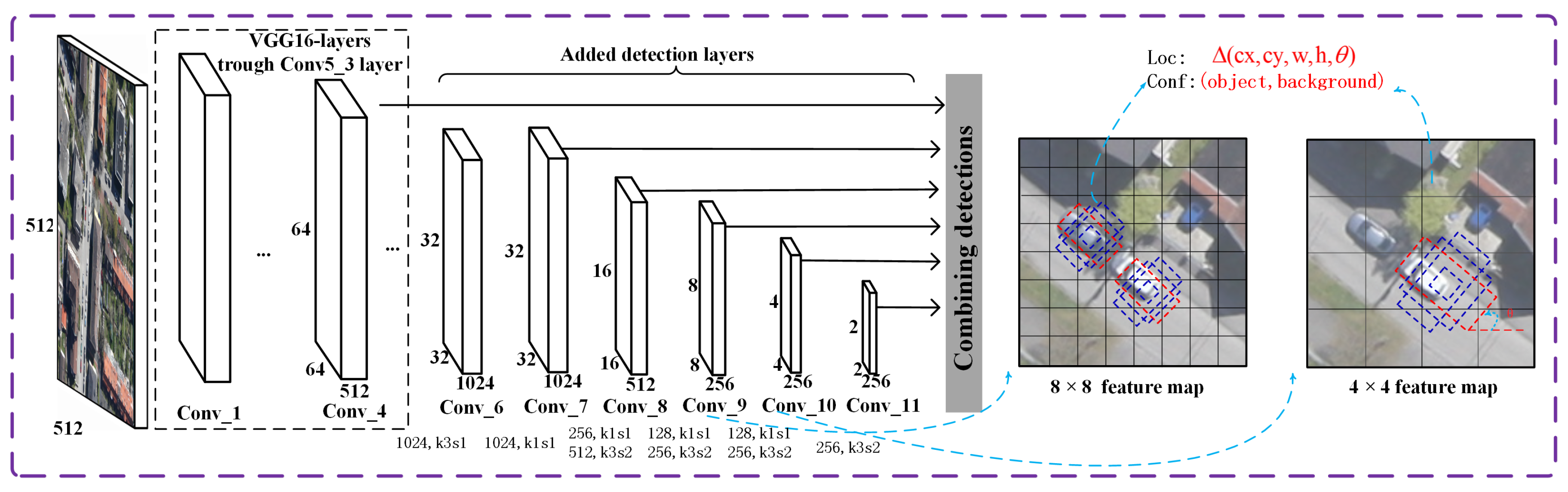
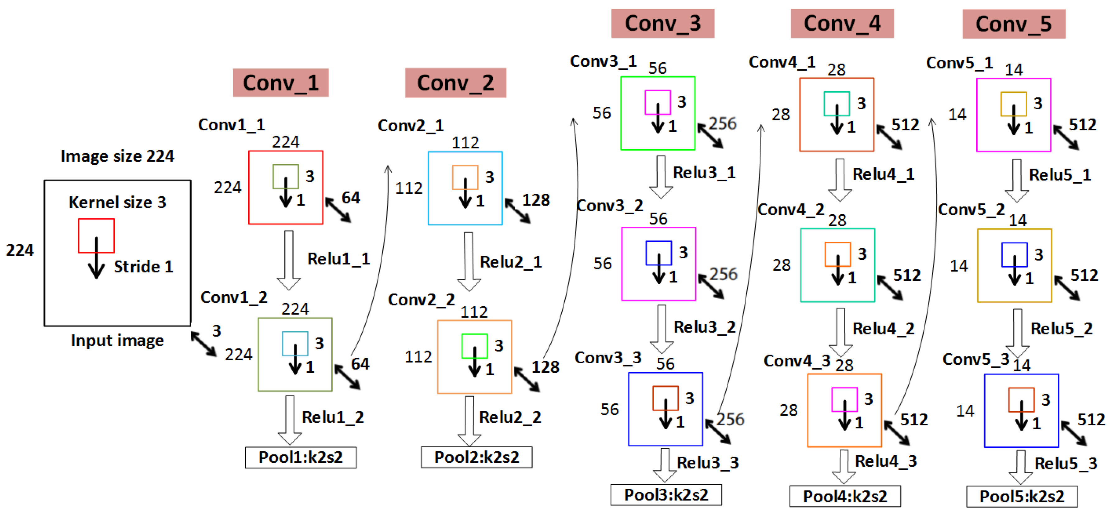
3.1. SSD
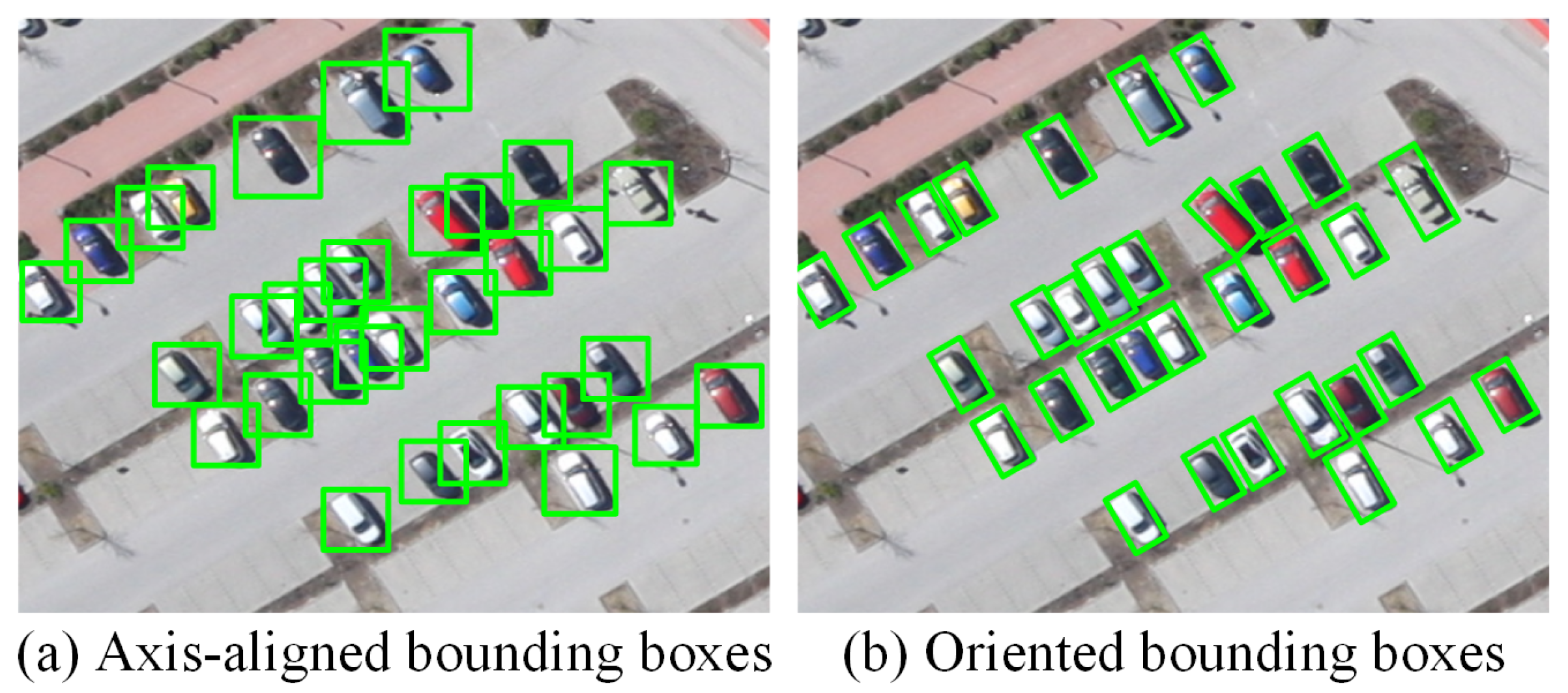
3.2. Oriented_SSD
3.3. Training
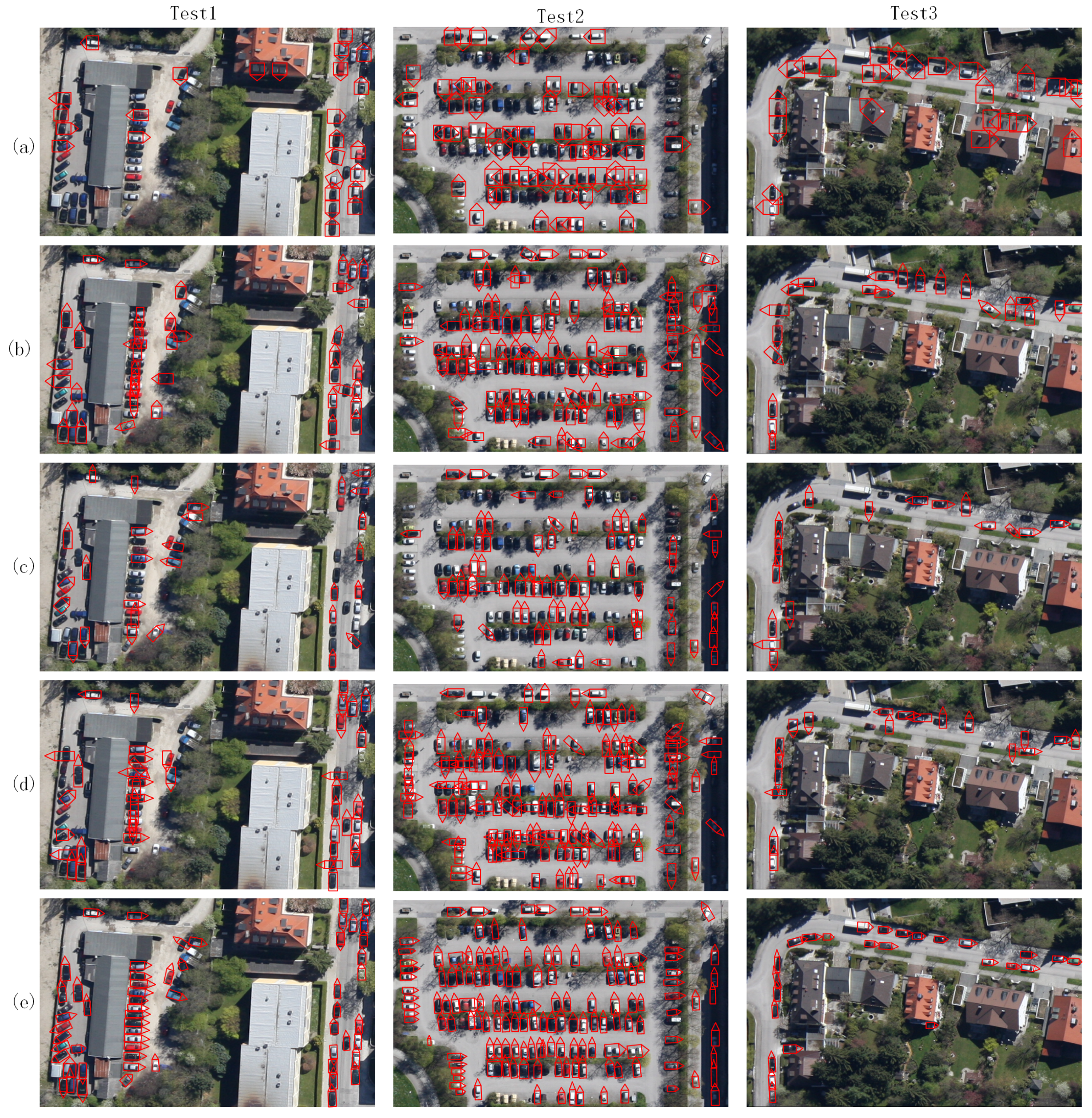
4. Experimental Results
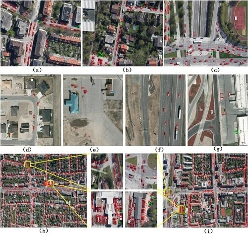
4.1. Dataset Description and Experimental Configuration
4.1.1. Dataset Description
4.1.2. Evaluation Metrics
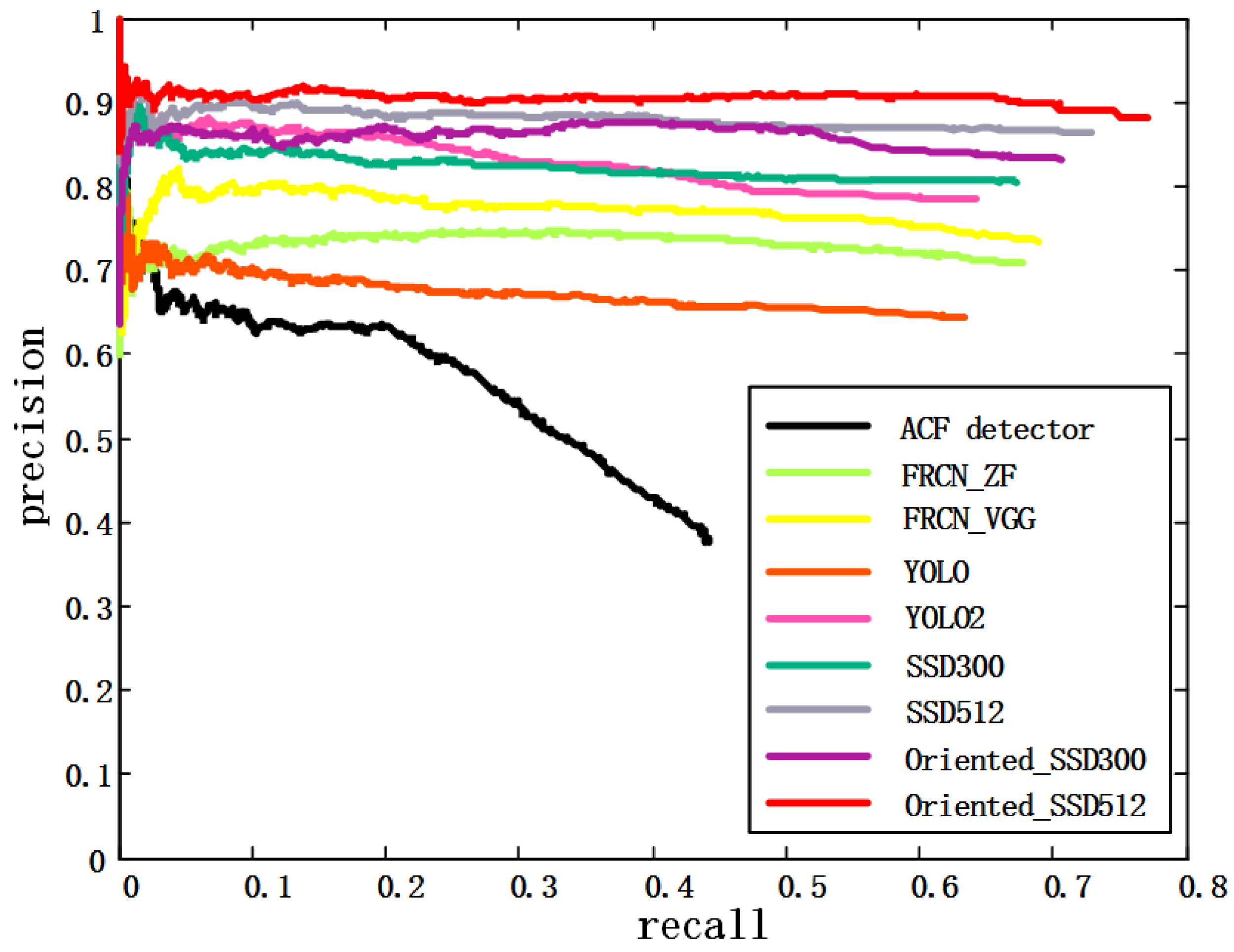
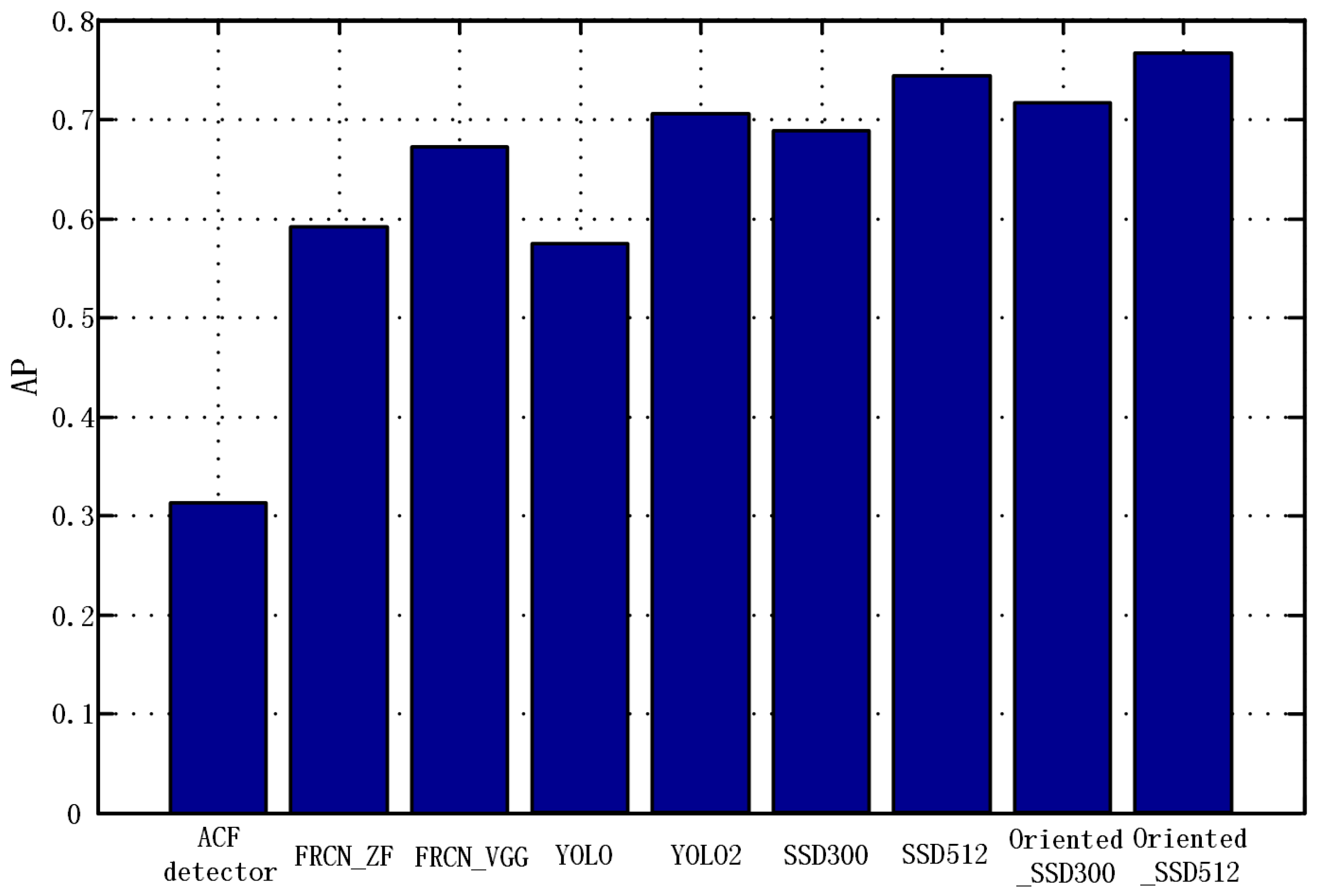
4.1.3. Compared Approaches
- ACF detector [35]: The aggregated channel feature (ACF) based detector is a traditional state-of-the-art method used in [2]. As a baseline, we use Piotr’s Computer Vision MATLAB Toolbox [36] implementation of the ACF detector. This binary detector was trained with a sliding window size of pixels and 2048 weak classifiers.
- Faster R-CNN [20]: This is a particularly influential detector. In our experiments, both the Zeiler and Fergus (ZF) model [15] and the VGG-16 model [16] are adopted as the feature extractor for detection, namely FRCN_ZF (ZF based Faster R-CNN, FRCN_ZF ) and FRCN_VGG (VGG-16 based Faster R-CNN, FRCN_VGG). The ZF model has five convolutional layers, and the VGG-16 model has 16 convolutional layers.
- SSD [14]: This is also an improvement of YOLO, which uses anchor boxes to predict bounding boxes from multiple feature maps with different resolutions. Following [14], we adopt the VGG-16 model as the feature extractor. Moreover, there are two configurations of SSD. SSD300 is trained with the image resized to , and SSD512 is trained with the image resized to . SSD512 has better performance than SSD300 in many detection tasks.
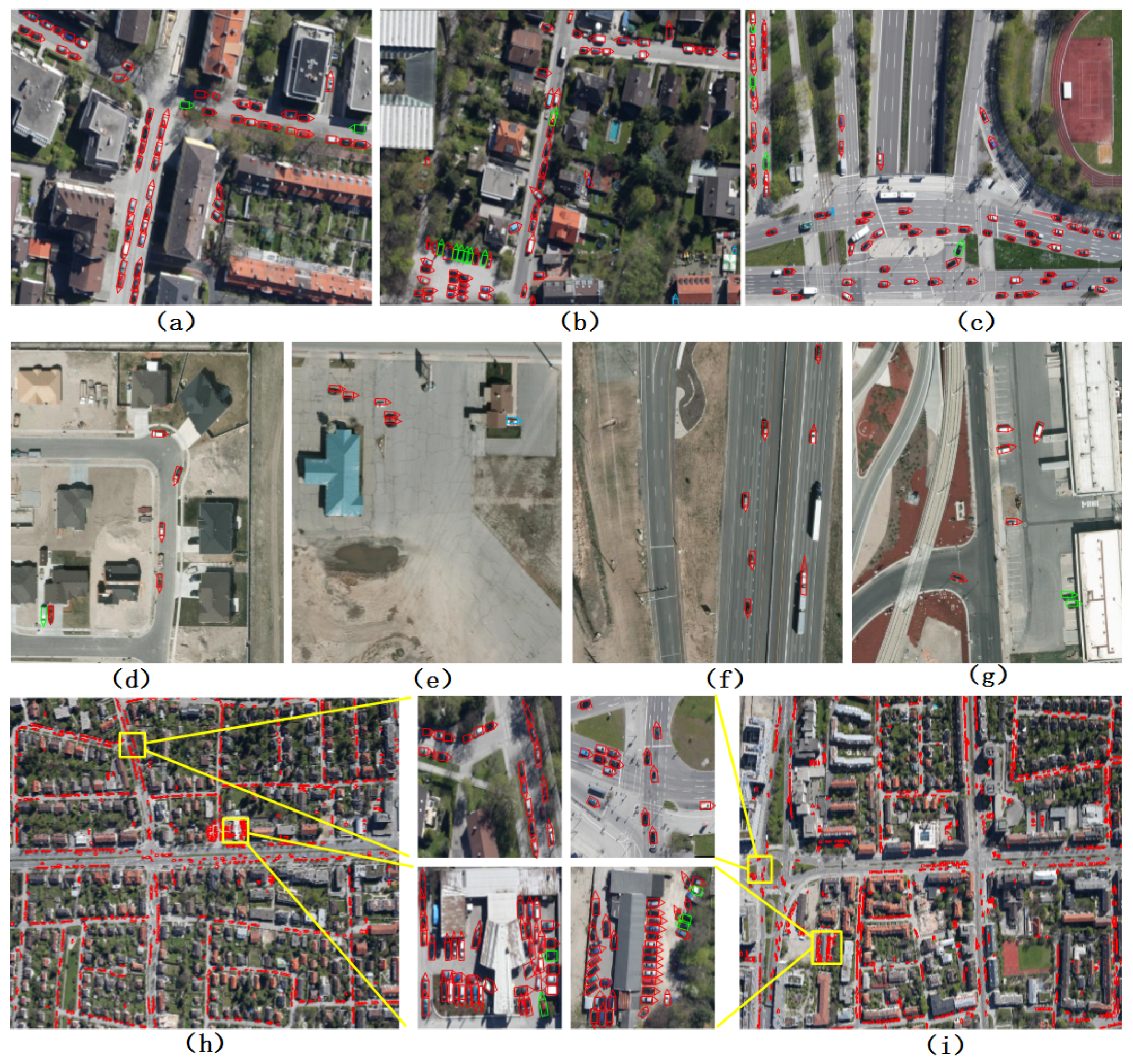
4.2. Results on DLR Vehicle Aerial Images
4.2.1. Evaluation of Vehicle Detection
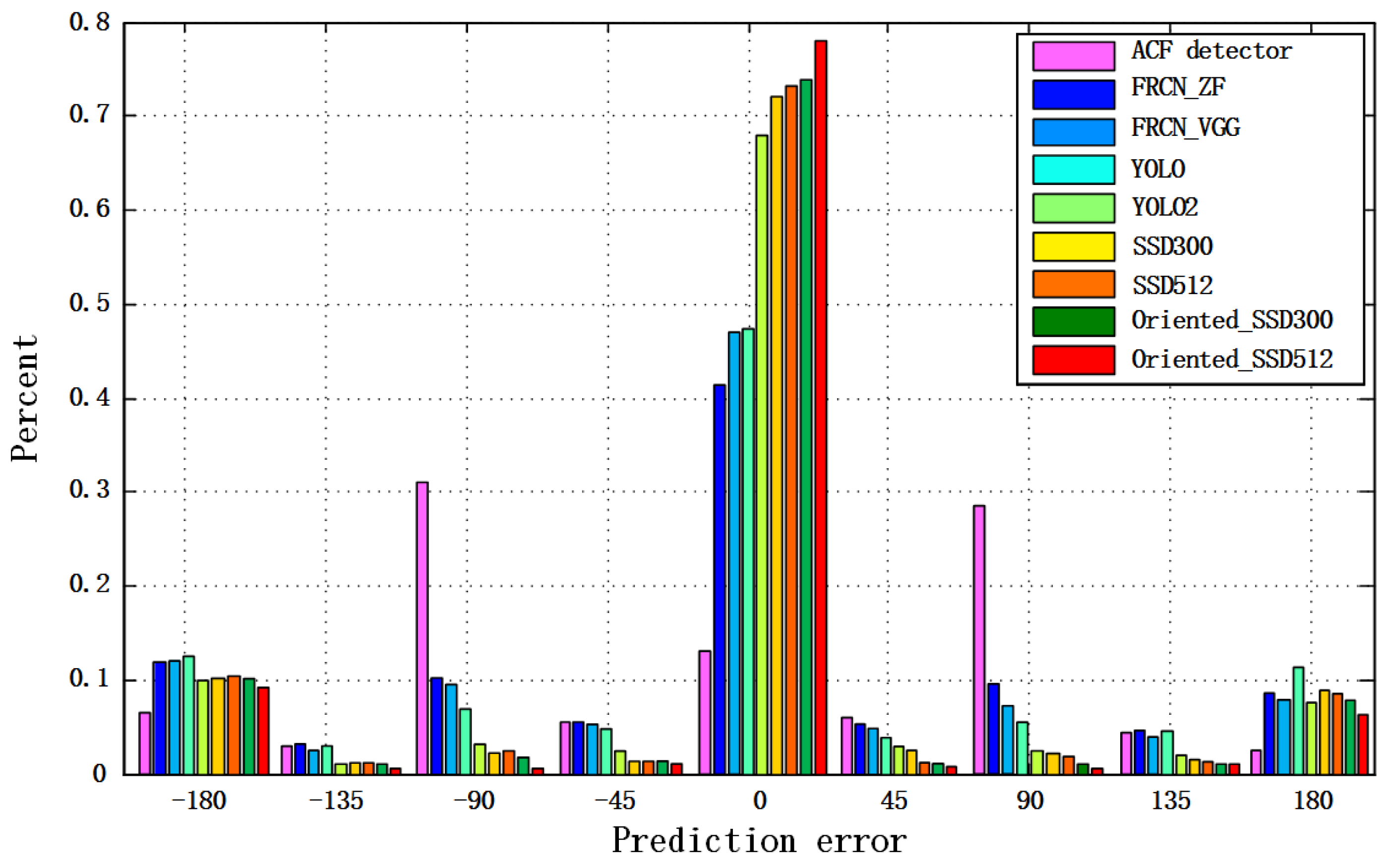
4.2.2. Evaluation of Orientation Estimation
4.3. Results on VEDAI Images
5. Conclusions
Acknowledgments
Author Contributions
Conflicts of Interest
References
- Leitloff, J.; Rosenbaum, D.; Kurz, F.; Meynberg, O.; Reinartz, P. An Operational System for Estimating Road Traffic Information from Aerial Images. Remote Sens. 2014, 6, 11315–11341. [Google Scholar] [CrossRef] [Green Version]
- Liu, K.; Mattyus, G. Fast multiclass vehicle detection on aerial images. IEEE Geosci. Remote Sens. Lett. 2015, 12, 1938–1942. [Google Scholar]
- Moranduzzo, T.; Melgani, F. Automatic car counting method for unmanned aerial vehicle images. IEEE Trans. Geosci. Remote Sens. 2014, 52, 1635–1647. [Google Scholar] [CrossRef]
- Moranduzzo, T.; Melgani, F. Detecting cars in UAV images with a catalog-based approach. IEEE Trans. Geosci. Remote Sens. 2014, 52, 6356–6367. [Google Scholar] [CrossRef]
- Chen, Z.; Wang, C.; Luo, H.; Wang, H.; Chen, Y.; Wen, C.; Yu, Y.; Cao, L.; Li, J. Vehicle Detection in High-Resolution Aerial Images Based on Fast Sparse Representation Classification and Multiorder Feature. IEEE Trans. Intell. Transp. Syst. 2016, 17, 2296–2309. [Google Scholar] [CrossRef]
- Cheng, H.Y.; Weng, C.C.; Chen, Y.Y. Vehicle detection in aerial surveillance using dynamic Bayesian networks. IEEE Trans. Image Process. 2012, 21, 2152–2159. [Google Scholar] [CrossRef] [PubMed]
- Shao, W.; Yang, W.; Liu, G.; Liu, J. Car detection from high-resolution aerial imagery using multiple features. In Proceedings of the IEEE International Geoscience and Remote Sensing Symposium (IGARSS), Munich, Germany, 22–27 July 2012; pp. 4379–4382. [Google Scholar]
- Kluckner, S.; Pacher, G.; Grabner, H.; Bischof, H.; Bauer, J. A 3D teacher for car detection in aerial images. In Proceedings of the IEEE International Conference on Computer Vision, Rio de Janeiro, Brazil, 14–21 October 2007; pp. 1–8. [Google Scholar]
- Kembhavi, A.; Harwood, D.; Davis, L.S. Vehicle detection using partial least squares. IEEE Trans. Pattern Anal. Mach. Intell. 2010, 33, 1250–1265. [Google Scholar] [CrossRef] [PubMed]
- Chen, Z.; Wang, C.; Wen, C.; Teng, X. Vehicle Detection in High-Resolution Aerial Images via Sparse Representation and Superpixels. IEEE Trans. Geosci. Remote Sens. 2015, 54, 1–14. [Google Scholar] [CrossRef]
- Chen, X.; Xiang, S.; Liu, C.L.; Pan, C.H. Vehicle Detection in Satellite Images by Hybrid Deep Convolutional Neural Networks. IEEE Geosci. Remote Sens. Lett. 2014, 11, 1797–1801. [Google Scholar] [CrossRef]
- Deng, Z.; Sun, H.; Zhou, S.; Zhao, J.; Zou, H. Toward Fast and Accurate Vehicle Detection in Aerial Images Using Coupled Region-Based Convolutional Neural Networks. IEEE J. Sel. Top. Appl. Earth Obs. Remote Sens. 2017, PP, 1–13. [Google Scholar] [CrossRef]
- Redmon, J.; Divvala, S.; Girshick, R.; Farhadi, A. You Only Look Once: Unified, Real-Time Object Detection. In Proceedings of the Computer Vision and Pattern Recognition, Las Vegas, NV, USA, 28–30 June 2016; pp. 779–788. [Google Scholar]
- Liu, W.; Anguelov, D.; Erhan, D.; Szegedy, C.; Fu, C.; Berg, A.C. Ssd: Single shot multibox detector. In Proceedings of the European Conference on Computer Vision, Amsterdam, The Netherlands, 8–16 October 2016; pp. 21–37. [Google Scholar]
- Zeiler, M.D.; Fergus, R. Visualizing and understanding convolutional networks. In Proceedings of the IEEE International European Conference on Computer Vision, Zurich, Switzerland, 6–12 September 2014; pp. 818–833. [Google Scholar]
- Simonyan, K.; Zisserman, A. Very deep convolutional networks for Large-Scale image recognition. arXiv, 2014; arXiv:1409.1556. [Google Scholar]
- Razakarivony, S.; Jurie, F. Vehicle detection in aerial imagery: A small target detection benchmark. J. Vis. Commun. Image Represent. 2016, 34, 187–203. [Google Scholar] [CrossRef]
- Girshick, R.; Donahue, J.; Darrell, T.; Malik, J. Region-based convolutional networks for accurate object detection and segmentation. IEEE Trans. Pattern Anal. Mach. Intell. 2016, 38, 142–158. [Google Scholar] [CrossRef] [PubMed]
- Girshick, R. Fast R-CNN. In Proceedings of the IEEE International Conference on Computer Vision, Boston, MA, USA, 8–10 June 2015; pp. 1440–1448. [Google Scholar]
- Ren, S.; He, K.; Girshick, R.; Sun, J. Faster R-CNN: Towards real-time object detection with region proposal networks. IEEE Trans. Pattern Anal. Mach. Intell. 2017, 39, 1137–1149. [Google Scholar] [CrossRef] [PubMed]
- Kim, K.H.; Hong, S.; Roh, B.; Cheon, Y.; Park, M. PVANET: Deep but Lightweight Neural Networks for Real-time Object Detection. arXiv, 2016; arXiv:1608.08021. [Google Scholar]
- Dai, J.; Li, Y.; He, K.; Sun, J. R-FCN: Object Detection via Region-based Fully Convolutional Networks. arXiv, 2016; arXiv:1605.06409v2. [Google Scholar]
- Cai, Z.; Fan, Q.; Feris, R.S.; Vasconcelos, N. A Unified Multi-scale Deep Convolutional Neural Network for Fast Object Detection. In Proceedings of the European Conference on Computer Vision, Amsterdam, The Netherlands, 8–16 October 2016; pp. 354–370. [Google Scholar]
- Redmon, J.; Farhadi, A. YOLO9000: Better, Faster, Stronger. arXiv, 2016; arXiv:1612.08242. [Google Scholar]
- Zheng, Z.; Zhou, G.; Wang, Y.; Liu, Y. A Novel Vehicle Detection Method With High Resolution Highway Aerial Image. IEEE J. Sel Top. Appl. Earth Obs. Remote Sens. 2013, 6, 2338–2343. [Google Scholar] [CrossRef]
- Li, F.; Lan, X.; Li, S.; Zhu, C.; Chang, H. Efficient vehicle detection and orientation estimation by confusing subsets categorization. In Proceedings of the IEEE International Conference on Computer and Communications, Chengdu, China, 14–17 October 2017; pp. 336–340. [Google Scholar]
- Uijlings, J.R.R.; Sande, K.E.A.V.D.; Gevers, T.; Smeulders, A.W.M. Selective Search for Object Recognition. Int. J. Comput. Vis. 2013, 104, 154–171. [Google Scholar] [CrossRef]
- Diao, W.; Sun, X.; Zheng, X.; Dou, F.; Wang, H.; Fu, K. Efficient saliency-based object detection in remote sensing images using deep belief networks. IEEE Geosci. Remote Sens. Lett. 2016, 13, 137–141. [Google Scholar] [CrossRef]
- Tuermer, S.; Kurz, F.; Reinartz, P.; Stilla, U. Airborne vehicle detection in dense urban areas using HoG features and disparity maps. IEEE J. Sel. Top. Appl. Earth Obs. Remote Sens. 2013, 6, 2327–2337. [Google Scholar] [CrossRef]
- Ševo, I.; Avramović, A. Convolutional neural network based automatic object detection on aerial images. IEEE Geosci. Remote Sens. Lett. 2016, 13, 740–744. [Google Scholar] [CrossRef]
- Qu, T.; Zhang, Q.; Sun, S. Vehicle detection from high-resolution aerial images using spatial pyramid pooling-based deep convolutional neural networks. Multimed. Tools Appl. 2016, 1–13. [Google Scholar] [CrossRef]
- Sommer, L.W.; Schuchert, T.; Beyerer, J. Fast Deep Vehicle Detection in Aerial Images. In Proceedings of the IEEE Winter Conference on Applications of Computer Vision, Santa Rosa, CA, USA, 24–31 March 2017; pp. 311–319. [Google Scholar]
- Deng, Z.; Lei, L.; Sun, H.; Zou, H.; Zhou, S.; Zhao, J. An enhanced deep convolutional neural network for densely packed objects detection in remote sensing images. In Proceedings of the IEEE International Workshop on Remote Sensing with Intelligent Processing, Shanghai, China, 18–21 May 2017; pp. 1–4. [Google Scholar]
- Chen, C.; Gong, W.; Hu, Y.; Chen, Y.; Ding, Y. Learning Oriented Region-based Convolutional Neural Networks for Building Detection in Satellite Remote Sensing Images. Int. Arch. Photogramm. Remote Sens. Spat. Inf. Sci. 2017, XLII-1/W1, 461–464. [Google Scholar] [CrossRef]
- Dollar, P.; Appel, R.; Belongie, S.; Perona, P. Fast Feature Pyramids for Object Detection. IEEE Trans. Pattern Anal. Mach. Intell. 2014, 36, 1532–1545. [Google Scholar] [CrossRef] [PubMed]
- Dollár, P. Piotr’s Computer Vision Matlab Toolbox (PMT). Available online: https://github.com/pdollar/toolbox (accessed on 27 September 2017).
- Tang, T.; Zhou, S.; Deng, Z.; Zou, H.; Lei, L. Vehicle Detection in Aerial Images Based on Region Convolutional Neural Networks and Hard Negative Example Mining. Sensors 2017, 17, 336. [Google Scholar] [CrossRef] [PubMed]


| Dataset | DLR Vehicle Aerial | VEDAI512 |
|---|---|---|
| #Images | 20 | 1246 |
| Image size | ||
| GSD (cm/pixel) | 13 | 25 |
| #Objects (car) | Train: 3191/Test: 5799 | 699 |
| #Objects/image | 449.5 | 1.11 |
| Mean width | 27.18 ± 9.09 | 16.7 ± 5.66 |
| Mean height | 25.56 ± 9.40 | 16.7 ± 5.84 |
| Method | Ground Truth | True Positive | False Positive | Recall Rate | Precision Rate | F1-Score | Time/per Image |
|---|---|---|---|---|---|---|---|
| ACF detector | 5799 | 3078 | 4062 | 53.08% | 43.31% | 0.47 | 6.29s |
| FRCN_ZF | 5799 | 3988 | 1082 | 68.77% | 78.66% | 0.73 | 5.76s |
| FRCN_VGG | 5799 | 4076 | 1017 | 70.30% | 80.03% | 0.75 | 11.32s |
| YOLO | 5799 | 3557 | 965 | 61.34% | 78.65% | 0.69 | 4.61s |
| YOLO2 | 5799 | 3877 | 914 | 66.86% | 80.92% | 0.74 | 4.22s |
| SSD300 | 5799 | 4005 | 985 | 69.06% | 80.26% | 0.74 | 4.61s |
| SSD512 | 5799 | 4400 | 844 | 75.88% | 83.91% | 0.79 | 5.22s |
| Oriented_SSD300 | 5799 | 4175 | 963 | 72.00% | 81.25% | 0.76 | 4.50s |
| Oriented_SSD512 | 5799 | 4572 | 773 | 78.84% | 85.53% | 0.82 | 5.17s |
| ACF Detector | FRCN_ZF | FRCN_VGG | YOLO | YOLO2 | SSD300 | SSD512 | Oriented_SSD300 | Oriented_SSD512 | |
|---|---|---|---|---|---|---|---|---|---|
| RMSE | 96.08 | 97.80 | 95.17 | 101.18 | 82.24 | 82.34 | 82.09 | 78.00 | 74.38 |
| W-Mean | 84.29 | 68.72 | 63.59 | 68.00 | 43.11 | 41.49 | 41.04 | 38.97 | 32.85 |
| Method | Ground Truth | True Positive | False Positive | Recall Rate | Precision Rate | F1-Score | Time/per Image |
|---|---|---|---|---|---|---|---|
| ACF detector | 1384 | 501 | 424 | 36.20% | 45.83% | 0.41 | 0.13s |
| FRCN_ZF | 1384 | 586 | 185 | 42.34% | 76.01% | 0.54 | 0.12s |
| FRCN_VGG | 1384 | 590 | 190 | 42.63% | 75.64% | 0.55 | 0.24s |
| YOLO | 1384 | 559 | 192 | 40.39% | 74.43% | 0.52 | 0.07s |
| YOLO2 | 1384 | 588 | 183 | 42.48% | 76.26% | 0.55 | 0.06s |
| SSD300 | 1384 | 589 | 180 | 42.56% | 76.59% | 0.55 | 0.07s |
| SSD512 | 1384 | 645 | 196 | 46.60% | 76.70% | 0.58 | 0.11s |
| Oriented_SSD300 | 1384 | 728 | 201 | 52.60% | 78.36% | 0.63 | 0.06s |
| Oriented_SSD512 | 1384 | 832 | 202 | 60.12% | 80.46% | 0.69 | 0.10s |
© 2017 by the authors. Licensee MDPI, Basel, Switzerland. This article is an open access article distributed under the terms and conditions of the Creative Commons Attribution (CC BY) license (http://creativecommons.org/licenses/by/4.0/).
Share and Cite
Tang, T.; Zhou, S.; Deng, Z.; Lei, L.; Zou, H. Arbitrary-Oriented Vehicle Detection in Aerial Imagery with Single Convolutional Neural Networks. Remote Sens. 2017, 9, 1170. https://doi.org/10.3390/rs9111170
Tang T, Zhou S, Deng Z, Lei L, Zou H. Arbitrary-Oriented Vehicle Detection in Aerial Imagery with Single Convolutional Neural Networks. Remote Sensing. 2017; 9(11):1170. https://doi.org/10.3390/rs9111170
Chicago/Turabian StyleTang, Tianyu, Shilin Zhou, Zhipeng Deng, Lin Lei, and Huanxin Zou. 2017. "Arbitrary-Oriented Vehicle Detection in Aerial Imagery with Single Convolutional Neural Networks" Remote Sensing 9, no. 11: 1170. https://doi.org/10.3390/rs9111170
APA StyleTang, T., Zhou, S., Deng, Z., Lei, L., & Zou, H. (2017). Arbitrary-Oriented Vehicle Detection in Aerial Imagery with Single Convolutional Neural Networks. Remote Sensing, 9(11), 1170. https://doi.org/10.3390/rs9111170