Using Copernicus Atmosphere Monitoring Service Products to Constrain the Aerosol Type in the Atmospheric Correction Processor MAJA

Abstract

The quantitative use of space-based optical imagery requires atmospheric correction to separate the contributions from the surface and the atmosphere. The MACCS (Multi-sensor Atmospheric Correction and Cloud Screening)-ATCOR (Atmospheric and Topographic Correction) Joint Algorithm, called MAJA, is a numerical tool designed to perform cloud detection and atmospheric correction. For the correction of aerosols effects, MAJA makes an estimate of the aerosol optical thickness (AOT) based on multi-temporal and multi-spectral criteria, but there is insufficient information to infer the aerosol type. The current operational version of MAJA uses an aerosol type which is constant with time, and this assumption impacts the quality of the atmospheric correction. In this study, we assess the potential of using an aerosol type derived from the Copernicus Atmosphere Monitoring Service (CAMS) operational analysis. The performances, with and without the CAMS information, are evaluated. Firstly, in terms of the aerosol optical thickness retrievals, a comparison against sunphotometer measurements over several sites indicates an improvement over arid sites, with a root-mean-square error (RMSE) reduced by 28% (from 0.095 to 0.068), although there is a slight degradation over vegetated sites (RMSE increased by 13%, from 0.054 to 0.061). Secondly, a direct validation of the retrieved surface reflectances at the La Crau station (France) indicates a reduction of the relative bias by 2.5% on average over the spectral bands. Thirdly, based on the assumption that surface reflectances vary slowly with time, a noise criterion was set up, exhibiting no improvement over the spectral bands and the validation sites when using CAMS data, partly explained by a slight increase in the surface reflectances themselves. Finally, the new method presented in this study provides a better way of using the MAJA processor in an operational environment because the aerosol type used for the correction is automatically inferred from CAMS data, and is no longer a parameter to be defined in advance.

1. Introduction

Time series of spaceborne high resolution optical images can be used to study the state and evolution of land surfaces. However, incoming sunlight and light reflected by the Earth’s surface can be scattered or absorbed by clouds, gas molecules, and aerosols [1,2]. Once cloud-contaminated observations have been detected and rejected, it is still difficult to separate the respective contributions from the surface and the atmosphere. A key step in processing such optical images is therefore the so-called atmospheric correction.

Several algorithms exist to process this atmospheric correction [3,4,5,6,7,8]. Most of them rely on multi-spectral criteria, based on empirical relationships between the surface reflectances at different spectral bands, to estimate the aerosol optical thickness (AOT). This is also the case of the algorithm described in [9], which is able to make an estimate of the aerosol type as well. This same method could be applied to Sentinel-2, but has not been used in practice and should be implemented in a future study.

In this article, we present a new version of the MACCS-ATCOR Joint Algorithm (MAJA), an atmospheric correction processor that first detects clouds and their associated shadows, then estimates the AOT, and finally performs the atmospheric correction. MAJA is based on the Multi-sensor Atmospheric Correction and Cloud Screening (MACCS) processor, developed by the Centre National d’Études Spatiales (CNES), and the Centre d’Études Spatiales de la Biosphère (CESBIO), and incorporates features from ATCOR (Atmospheric and Topographic Correction) [7,8], developed by the German Aerospace Centre (DLR). Complete details about the MACCS method can be found in [10]. The absorption by air molecules is modeled using the Simplified Model for Atmospheric Correction (SMAC) [11]. Regarding the aerosol contribution, MAJA estimates the AOT using multi-temporal [12] and multi-spectral criteria as described in [3,4,5,6,13,14]. Based on this AOT estimate, and using a radiative transfer code [15], MAJA can convert top-of-atmosphere (TOA) reflectances into surface reflectances.

Estimating the aerosol type using these techniques increases the noise in the surface reflectance time series because of the limited independent information. Thus, until now, MAJA has been using an aerosol type that is constant with time, which only depends on the type of site being processed. However, a good estimate of the dominant aerosol types present in the image is important because of the high temporal and spatial variability of absorption and optical properties of the various existing aerosol types [16] and their variable impact on the reflectance for a given AOT. A wrong choice of the aerosol type and its optical properties (scattering and absorption) will result in large estimation errors of the AOT and in the corrected surface reflectances.

In this study, we explore the possibility of improving the estimation of the AOT, using additional external information on the aerosol types. Several forecasting systems provide aerosol products, such as Goddard Earth Observing System (GEOS) [17] or the NOAA (National Oceanic and Atmospheric Administration) Environmental Modeling System (NEMS) [18], both relying on the Georgia Tech/Goddard Global Ozone Chemistry Aerosol Radiation and Transport (GOCART) model [19]. The Community Earth System Model (CESM)) [20] and Navy Operational Global Analysis Prediction System (NOGAPS) [21] also provide these types of products, using respectively the Community Aerosol and Radiation Model for Atmospheres (CARMA) [22] and Navy Aerosol Analysis and Prediction System (NAAPS) [23,24,25] models. We chose to use the Copernicus Atmosphere Monitoring Service (CAMS) products [26,27], mainly because we had direct access to accurate information from CAMS project members who are also part of this study, and because of the operational status of CAMS and the simple access to its products. The CAMS system uses the Composition-Integrating Forecasting System (C-IFS) model and provides global analysis and forecasts of AOT and optical properties for the five following aerosol types: Sulfate, Organic Matter, Black Carbon, Sea Salt, and Dust. The C-IFS model includes static or dynamical emissions and represents transport as well as sedimentation and wet and dry deposition. The sources of anthropogenic aerosols (Sulfate, Organic Matter and Black Carbon) are provided by external datasets such as the Global Fire Emission Database (GFED) [28,29], Speciated Particulate Emission Wizard (SPEW) [30] and the Emission Database for Global Atmospheric Research (EDGAR) [31]. On the other hand, the sources of natural aerosols (Sea Salt and Dust) come from C-IFS model parameters such as wind speed or soil moisture for instance. AOT from the Moderate Resolution Imaging Spectroradiometer (MODIS) instrument [13,27] on board the Aqua and Terra satellites are assimilated. Using CAMS forecasts allows the determination of the dominant aerosols, and thus can help us choose the appropriate aerosol optical properties in our processor. Another possibility would have been to directly use the total AOT predicted by CAMS. However, because of the complexity of the processes involved in the C-IFS model, the incomplete information coming from MODIS (no data on the vertical distribution), and the absence of observations for cloudy scenes, it seemed relevant not to rely on CAMS for the AOT. Besides, the AOT forecasts from CAMS were not reliable enough (root-mean-square error, RMSE = 0.176) when compared to the Aerosol Robotic Network (AERONET) observations of summer 2016 [32]. Considering the high temporal variability of the AOT, the AOT estimated by the MAJA processor is potentially more accurate because it is processed on the current image, whereas the AOT from CAMS is a forecast. As a consequence, we decided to only use the information about the aerosol type coming from CAMS.

The interest of using CAMS products was assessed using Sentinel-2A time series. Sentinel-2A is an optical high-resolution Earth observation satellite. It provides, with a 10-day repetitivity, global coverage of land surfaces and high quality data for operational land monitoring [33]. The AOT calculated by MAJA (using CAMS products to constrain the AOT estimation) was compared to ground-based data from the Cimel sunphotometers comprising the AERONET network [34,35]. Direct validation of surface reflectances was performed on a particular site using ground-based observations. Finally, as surface reflectances are assumed to be relatively stable with time, a criterion was defined to assess if the noise in the surface reflectances time series after atmospheric correction was reduced when using better-suited aerosol optical properties (deduced from CAMS information).

After a description of the methods and of the different datasets, this paper presents the results and evaluates the performances of the tool, either with or without using CAMS information.

2. Methods and Datasets

2.1. Atmospheric Correction with MAJA

MAJA is a multi-mission atmospheric correction processor used to process time series of high resolution images, such as those acquired by Sentinel-2 (at 10-, 20-, and 60-m resolution depending on the spectral band). It provides a cloud mask (and the associated shadows) and a water and snow mask, as well as an estimation of the aerosol optical thickness (AOT), and produces as the final output time series of surface reflectance.

The estimation of the AOT is computed thanks to a combination of multi-temporal and multi-spectral criteria. The multi-temporal criterion relies on the relative stability of surface reflectances with time (within a few days), compared to the high variability of AOT (which can change hourly). The changes of measured reflectances on consecutive images are then attributed to changes of AOT, and the contributions from the surface and the atmosphere can then be separated. The case when the AOT is nearly the same between these two images is also taken care of, and a Levenberg–Marquardt non-linear least mean squares fitting is performed to search for the AOT, which minimizes the cost function described in [10]. This multi-temporal criterion will take advantage of the five-day repetitivity when both Sentinel-2 satellites are operating simultaneously [33], but it is already providing good results for Sentinel-2A alone and Landsat-8 alone. The multi-spectral criterion assumes a relationship between the blue (444 nm) and the red (664 nm) surface reflectances:

$${\rho }_{blue}=0.45\times {\rho }_{red}$$

(1)

The coefficient used in [10] for this relationship was 0.568 for Landsat-5 and 0.479 for Landsat-7. Initially in MAJA, the first value to be used was 0.55, but after some adjustments the value of 0.45 was found to give better performances. Based on this relationship, the multi-spectral method searches for the AOT, which minimizes the difference between the surface reflectance in the blue band after atmospheric correction and the blue surface reflectance predicted by the relationship.

A combination of the multi-temporal and the multi-spectral methods is finally performed, with the weight of the multi-temporal method depending on the repetitivity of the dates available. A complete description of the criteria, the methods, and the cost functions can be found in [10].

In the previous versions of the MAJA processor, the aerosol type was a parameter. It was constant with time and was defined prior to any processing according to the surface type. In practice, the same aerosol type was used everywhere: a standard continental aerosol type, inspired by [16]. It is described by a log-normal size distribution, with the following parameters:

• No coarse mode, and a modal radius $r_0=0.2$ $\mathsf{\mu }$m for the fine mode
• Geometric standard deviation $\sigma =1.82$
• A refractive index with a real part of 1.53, and a spectrally variable imaginary part as shown in

  Table 1. Imaginary part of refractive index (×1000) of the standard continental aerosol type, for Sentinel-2A bands.

  Band	B1	B2	B3	B4	B5	B6	B7	B8	B8a	B9	B10	B11	B12
  [nm]	444	496	560	664	704	740	782	832	865	944	1373	1613	2198
  	−1.00	−0.75	−0.50	−0.10	−0.10	−0.10	−0.10	−0.10	−0.10	−0.10	−0.10	−0.10	−0.10

This aerosol type was defined to optimize the performances of MAJA over vegetated continental surfaces. Although it was intended to use other aerosol types for other surface types, it has not been attempted in practice.

Before using MAJA, a look-up table (LUT) is computed for the aerosol type which will be used. This LUT is generated by the Successive Orders of Scattering (SOS) radiative transfer model [15] and provides the surface reflectance value corresponding to a top-of-atmosphere (TOA) reflectance value. The LUT is parameterized by the viewing geometry, the surface altitude, the wavelength, and of course the AOT.

2.2. Copernicus Atmosphere Monitoring Service (CAMS)

2.2.1. About CAMS and Its Products

Copernicus is the European Union’s program for environment monitoring, with a strong satellite Earth observation component. The Copernicus Atmosphere Monitoring Service (CAMS) operates within the scope of this program and provides products describing air quality and atmospheric composition, climate forcing, ozone layer, solar radiation, emissions, and surface fluxes. It is operated operationally and the data is made freely available by the European Centre for Medium-Range Weather Forecasts (ECMWF).

Among these products, analysis and forecasts of aerosol optical thickness at 550 nm for five different aerosol types are provided by the forward model C-IFS assimilating data from the MODIS instruments on the Aqua and Terra satellites [27]. Polar Multi-Sensor Aerosol Product (PMAp) data from the European Organisation for the Exploitation of Meteorological Satellites (EUMETSAT) is also assimilated, but not for the period analyzed in this study. The five aerosol types in C-IFS are Organic Matter, Sulfate, Sea Salt, Dust, and Black Carbon [26,36].

The data used in this study comes from the near-real-time dataset. For each day, the three-hour forecast based on the analysis (assimilation of MODIS data) at 00:00 UTC (Coordinated Universal Time) is used (i.e., 03:00 UTC), as well as the three-hour forecast based on the analysis at 12:00 UTC (i.e., 15:00 UTC, available from 21 June 2016). Finally, the data is downloaded and interpolated on a regular grid with a spatial resolution of 1.25${}^{\circ }$, from a Gaussian native grid with a resolution of 0.4${}^{\circ }$ (0.8${}^{\circ }$ before June 2016).

In this study we used the aerosol optical thickness at 550 nm for the five aerosol types, the relative humidity at 23 different pressure levels, and the mass mixing ratios at 60 different model levels.

Figure 1 shows an example of the forecast AOT from CAMS, for four aerosol types.

2.2.2. Optical Properties of CAMS Aerosols

The aerosol types of natural origin such as Sea Salt and Dust are each represented by three size bins. The Organic Matter is described with two components (hydrophilic and hydrophobic) and the Sulfate is described using only one variable [26]. The physical and optical properties at 550 nm for these aerosol types are provided in

Table 2. CAMS (Copernicus Atmosphere Monitoring Service) aerosols optical properties at 550 nm and 80% relative humidity (RH). $r_0$ is the modal radius, $\sigma$ is the geometric standard deviation, ${\alpha }_e$ is the mass extinction coefficient and $\omega$ is the single scattering albedo.

Aerosol Type	${\mathit{r}}_0$ ($\mathsf{\mu }$m)	$\mathit{\sigma }$	${\mathit{\alpha }}_{\mathit{e}}$ (m${}^2$·g${}^{-1}$)	Refractive Index	$\mathit{\omega }$
Sea Salt (0.03–0.5 $\mathsf{\mu }$m)	0.1992 and 1.992	1.9 and 2.0	6.67	1.44−$0.0006$ i	0.999
Sea Salt (0.5–5 $\mathsf{\mu }$m)			0.50		0.986
Sea Salt (5–20 $\mathsf{\mu }$m)			0.15		0.982
Dust (0.03–0.55 $\mathsf{\mu }$m)	0.29	2.0	2.63	1.48−$0.0016$ i	0.990
Dust (0.55–0.9 $\mathsf{\mu }$m)			0.87		0.967
Dust (0.9–20 $\mathsf{\mu }$m)			0.43		0.944
Organic Matter hydrophilic	0.0527	2.0	8.62	1.40−$0.0000$ i	1
Organic Matter hydrophobic	0.0355	2.0	3.07	1.52−$0.0000$ i	1
Black Carbon	0.0118	2.0	9.51	1.75−$0.4500$ i	0.208
Sulfate	0.0527	2.0	11.89	1.40−$0.0000$ i	1

.

The mass extinction coefficients ${\alpha }_e$ were generated from the refractive indices using the Mie theory, as described in [37,38]. They will be used in Section 2.3.2 to compute the average relative humidity (RH) of the atmospheric column, weighted at each layer by the AOT computed from the mass mixing ratios (expressed in kilograms of aerosol per kilograms of dry air) and the extinction coefficients. The use of the Mie theory on the Dust aerosol type, despite being much simpler from a computational point of view, is inappropriate due to the Dust particles being non-spherical. An estimation of the uncertainty caused by using the Mie theory on non-spherical particles is given in [39,40], where a large difference between spherical and non-spherical particles appears regarding the phase function in the range 90–${180}^{\circ }$. The choice of using the Mie theory in our LUT computations was made in order to be consistent with the use of the Mie theory within CAMS. However, using an alternative such as the T-matrix method [41] should be the subject of a future study. A mono-modal log-normal size distribution is used for every aerosol type, except for Sea Salt, which is described with a bimodal distribution. For Sea Salt, the number concentrations for the first and second mode are 70 and 3 cm${}^{-3}$, respectively [36]. The Sea Salt, Sulfate, and Organic Matter hydrophilic types depend on the relative humidity (RH), unlike the Dust, Black Carbon, and Organic Matter hydrophobic types which keep the same properties independently of the RH values.

Some assumptions are made in CAMS for specific aerosol types. The Sulfate aerosol is assumed to be non-absorbing (pure scattering). The modal radius and refractive indices of hydrophilic Organic Matter are identical to those of Sulfate. The optical properties of hydrophobic Organic Matter are independent of the RH and correspond to those of hydrophilic Organic Matter at RH = 0%. The refractive indices of Sea Salt are independent of the wavelength, and so is the real part of the refractive indices of Dust. The Black Carbon refractive indices are independent of the wavelength and relative humidity, and there is no distinction between hydrophilic and hydrophobic Black Carbon yet in the current version of CAMS.

As we will see in Section 3.1, the refractive indices used in this study are different from the ones in CAMS for the Dust (1.53–−0.0052 i instead of 1.48−0.0016 i at 550 nm) and Black Carbon (1.75–0.20 i instead of 1.75–0.45 i at 550 nm) aerosols.

2.2.3. Aerosol Dependency on Relative Humidity

As previously presented, the Sea Salt, Sulfate, and Organic Matter types depend on the relative humidity (RH). These aerosol types should then be described for a set of sampling values of RH. For this paper, we chose the following set of values, for which the optical properties (modal radius, ${\alpha }_e$ and refractive index) are described:

$$RH=[30,50,70,80,85,90,95]$$

The first value is 30% because the deliquescence (the point where an aerosol particle starts holding water molecules, going from the solid to the liquid phase and increasing in size) appears around 40%, meaning that the optical properties are supposed to be constant with RH varying from 0 to 30% [42]. The last sampling value is 95% because beyond this value, the optical properties are difficult to estimate and a cloud might be involved. If the actual RH value is higher than 95%, the LUT corresponding to RH = 95% is used. The step of 20% for the first sampling values was chosen to avoid handling too many LUTs and because the error made with this 20% step was small. For the last sampling values, the step was reduced to 10% and 5% because the optical properties vary quickly when the RH values are large.

2.3. Using CAMS Products to Constrain the Aerosol Type in MAJA

2.3.1. Using Five Aerosol Types Instead of One

Instead of using the constant aerosol type, as in the original version of MAJA, our idea is to use the five aerosol types available within CAMS and to determine their contribution using their respective AOTs from CAMS. The AOTs of the five aerosol types at the coordinates of the image centre are computed by a linear interpolation using the four closest neighbours in the CAMS regular grid. All of this is done with the two CAMS dates surrounding the Sentinel-2 overpass time, within a 24-h window. These two datasets are used to compute a temporal linear interpolation, weighted according to the Sentinel-2 overpass time. We then compute a linear interpolation of the five look-up tables (previously computed for each one of the aerosol types), with the weight of each LUT being the proportion (based on the AOT at the image centre and at the Sentinel-2 overpass time) of the corresponding aerosol type. This interpolated LUT is finally used by the MAJA processor to provide us with the surface reflectance corresponding to the TOA reflectance.

Regarding the temporal interpolation, if only one CAMS date is available within the 24-h window, no temporal interpolation is performed, and the data are used from the only CAMS date available. Finally, if no CAMS date is available at all, the constant aerosol type defined in Section 2.1 is used, as in the previous configuration of MAJA.

As shown in Section 2.2.2, the Black Carbon type has very high absorption, leading to extreme optical properties. In practice, Black Carbon is always mixed with other aerosol types, such as Organic Matter or Sulfate. Since we feared Black Carbon absorption was exaggerated, we also tested the integration of CAMS data where the linear interpolation of the LUT is performed only with the four remaining aerosol types: Sea Salt, Sulfate, Organic Matter and Dust.

In Section 3, comparisons are presented to evaluate whether or not using CAMS data improves the performances of the AOT estimation and of the atmospheric correction.

2.3.2. Choosing the Appropriate LUT as a Function of RH

As introduced previously, a look-up table (LUT) is computed for each aerosol type, and also for a set of RH sampling values (defined in Section 2.2.3) for the aerosols which depend on RH. In order to use the right LUTs, the effective relative humidity has to be computed. To do so, the RH vertical profile is determined at the image centre by a linear interpolation using the RH data of the four closest neighbours in the CAMS regular grid. The effective RH at the image centre is then calculated as the average of the vertical profile, weighted by the AOT of each layer.

The AOT of each layer (model level), used to weight the average RH, is computed as follows:

• for each RH-dependent aerosol type (Sea Salt, Sulfate and hydrophilic Organic Matter), ${\alpha }_e$ corresponding to the RH of the model level is interpolated. For the other types (Dust, Black Carbon and hydrophobic Organic Matter), the constant value of ${\alpha }_e$ is used.
• the AOT of the model level is finally calculated as the sum of the optical depth of the five aerosol types:

  $$\tau \left(l\right)=\sum _{a=1}^5{\tau }_a\left(l\right)$$

  (2)

  where $\tau \left(l\right)$ is the AOT of the model level l, and ${\tau }_a\left(l\right)$ is the AOT due to each aerosol type a at model level l. ${\tau }_a\left(l\right)$ is calculated differently according to the aerosol type:

  -

  for Dust and Sea Salt, because they are described with three size bins, their mass mixing ratios (provided by CAMS) and their mass extinction coefficients are different according to the bin:

  $${\tau }_a\left(l\right)=\sum _{bin=1}^3{\alpha }_{e_{bin}}(a,l)\times C_{bin}(a,l)\times \left[P\left(l\right)-P(l+1)\right]\times {\mathrm{g}}^{-1}$$

  (3)

  where $\mathrm{g}=9.81$ m·s${}^{-2}$ is the gravity, P is the atmospheric pressure at the interface of model level l, and ${\alpha }_{e_{bin}}(a,l)$ and $C_{bin}(a,l)$ are the mass extinction coefficient and mass mixing ratio, respectively, of aerosol a at model level l.

  -

  for Sulfate and Black Carbon, as they are described with only one component,

  $${\tau }_a\left(l\right)={\alpha }_e(a,l)\times C(a,l)\times \left[P\left(l\right)-P(l+1)\right]\times {\mathrm{g}}^{-1}$$

  (4)

  -

  for Organic Matter, we sum its two components (hydrophilic and hydrophobic, as described in Table 2):

  $${\tau }_a\left(l\right)=\sum _{comp=hydrophilic}^{hydrophobic}{\alpha }_{e_{comp}}(a,l)\times C_{comp}(a,l)\times \left[P\left(l\right)-P(l+1)\right]\times {\mathrm{g}}^{-1}$$

  (5)

The average RH is then calculated as follows:

$$R{H}_{average}=\sum _{l}RH\left(l\right)\times \frac{\tau \left(l\right)}{\tau }$$

(6)

where $RH\left(l\right)$ is the RH value corresponding to the model level l, $\tau \left(l\right)$ is defined in Equation (2), and $\tau$ is the total AOT of the vertical profile:

$$\tau =\sum _l\tau \left(l\right)$$

(7)

This $R{H}_{average}$ is computed for both surrounding CAMS dates, as explained in Section 2.3.1. The temporal linear interpolation, weighted according to the Sentinel-2 overpass time, is performed to provide the final average RH. In the end, for the aerosol types depending on the relative humidity, the LUT used is the one whose RH sampling value is the closest to the final average RH.

2.4. Dataset

Sentinel-2 [33] is an Earth observation mission operated by the European Space Agency (ESA) and is part of the Copernicus program. This mission consists of the two satellites Sentinel-2A and Sentinel-2B which will soon offer high repetitivity data with a 5-day revisit period as well as a constant viewing angle and global coverage of land surfaces. Sentinel-2A was launched on 23 June 2015 and Sentinel-2B on 7 March 2017. They follow a Sun-synchronous orbit with a 786-km altitude and an overpass time at the descending node at 10:30 a.m. local time. Sentinel-2 provides data over 13 spectral bands, ranging from the visible spectrum to the near-infrared (NIR) and short-wave infrared (SWIR) spectra. The data used for this paper only come from the Sentinel-2A satellite which has a nominal repetitivity of 10 days. However we used adjacent orbits, when available, to increase this frequency to the following revisit scheme starting from day d: d, $d+3$, $d+10$, $d+13$, $d+20$, $d+23$, etc. By doing so we allowed the multi-temporal method to be more reliable by using more frequent observations. At the same time, it also led to the introduction of a slight uncertainty due to different observation angles. However, when estimating the AOT, a directional correction was applied to account for the different viewing conditions of the adjacent orbits, using the method from [43] and the coefficients from [44].

The sites presented in

Table 3. Sites used in this study from the Aerosol Robotic Network (AERONET) [34,35] network.

Site	Latitude	Longitude	Type	AERONET Sites
Ben Salem (Tunisia)	35.55${}^{\circ }$N	9.91${}^{\circ }$E	arid	Ben Salem
Badajoz (Spain)	38.88${}^{\circ }$N	7.01${}^{\circ }$W	arid	Badajoz
Banizoumbou (Niger)	13.54${}^{\circ }$N	2.66${}^{\circ }$E	arid	Banizoumbou
Ouarzazate (Morocco)	30.93${}^{\circ }$N	6.91${}^{\circ }$W	arid	Ouarzazate, Saada
Sede Boker (Israel)	30.86${}^{\circ }$N	34.78${}^{\circ }$E	arid	SEDE BOKER
Pretoria (South Africa)	25.76${}^{\circ }$S	28.28${}^{\circ }$E	arid	Pretoria CSIR DPSS
Mongu (Zambia)	15.27${}^{\circ }$S	23.13${}^{\circ }$E	arid	Mongu Inn
Carpentras (France)	44.08${}^{\circ }$N	5.06${}^{\circ }$E	vegetated	Carpentras
Zaragoza (Spain)	41.63${}^{\circ }$N	0.88${}^{\circ }$W	vegetated	Zaragoza
Sirmione (Italy)	45.50${}^{\circ }$N	10.61${}^{\circ }$E	vegetated	Sirmione Museo GC, Modena
Montsec (Spain)	42.05${}^{\circ }$N	0.73${}^{\circ }$E	vegetated	Montsec, Barcelona
Toulouse (France)	43.57${}^{\circ }$N	1.37${}^{\circ }$E	vegetated	Toulouse MF
Kishinev (Moldova)	47.00${}^{\circ }$N	28.82${}^{\circ }$E	vegetated	Moldova
Alta Floresta (Brazil)	9.87${}^{\circ }$S	56.10${}^{\circ }$W	vegetated	Alta Floresta
Marbel (Philippines)	6.50${}^{\circ }$N	124.84${}^{\circ }$E	vegetated	ND Marbel Univ

and Figure 2 were selected because they are affected by a wide range of aerosol types described in CAMS, and because long-enough time series of AERONET data were available. Besides, Sentinel-2 offers a better repetitivity over Europe and Africa. The time series used in this paper range from 1 April 2016, when Sentinel-2A acquisitions started to be steadily available, to 15 October 2016.

3. Results and Discussion

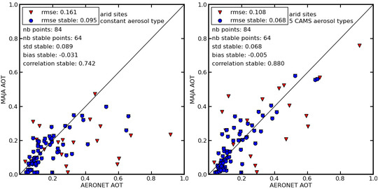
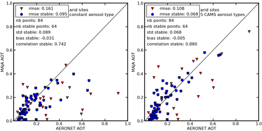
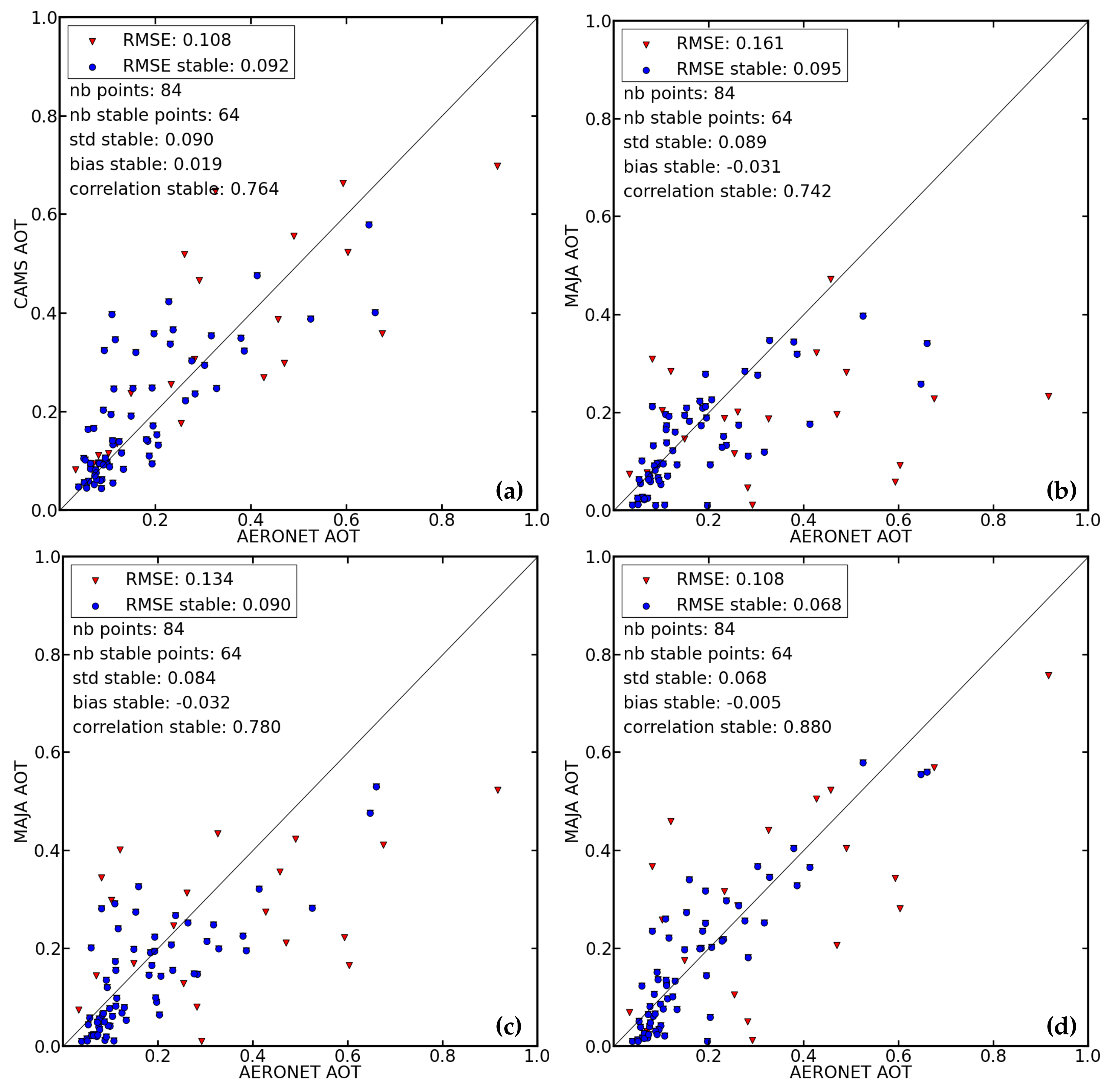
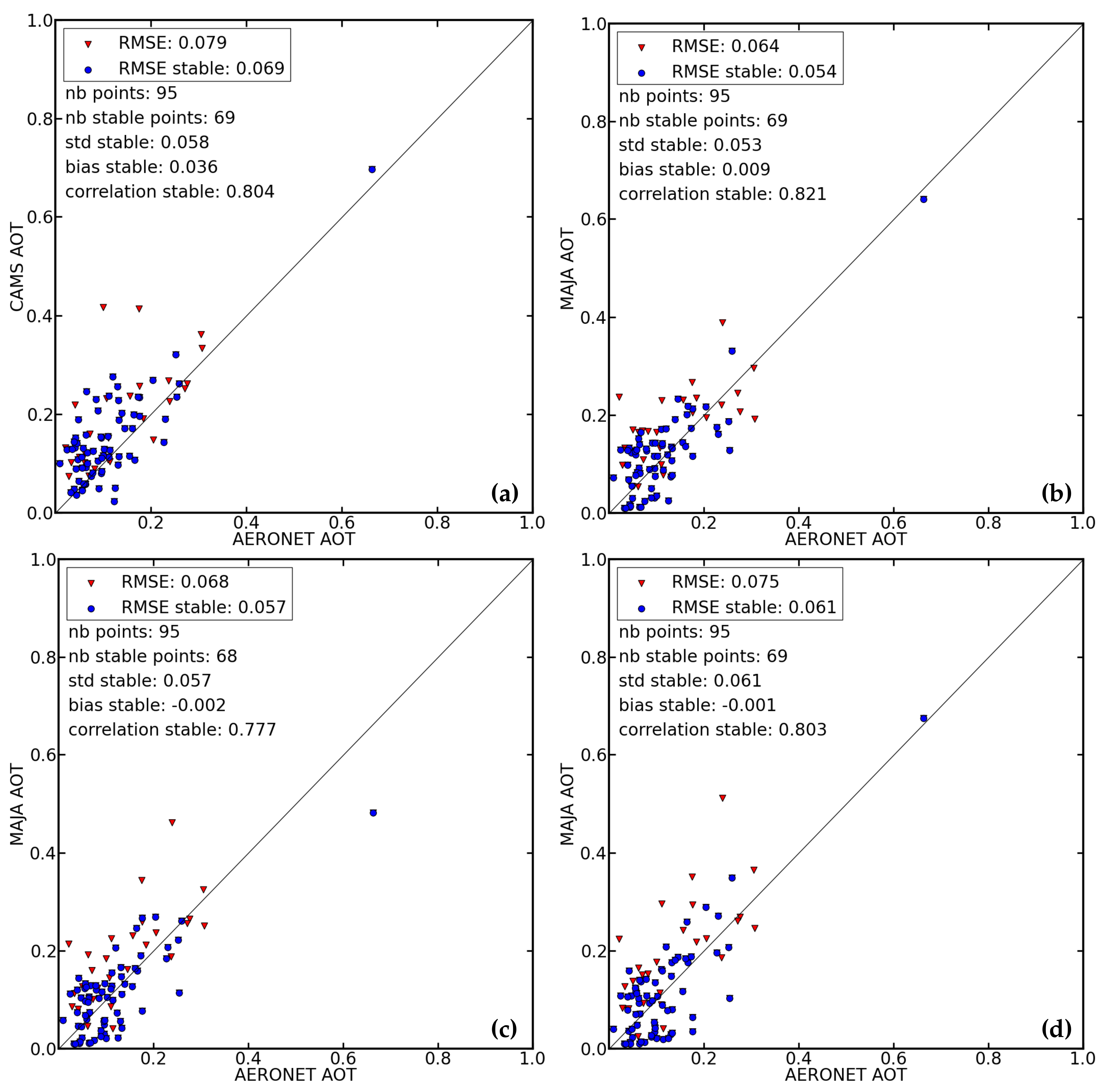
3.1. Validation of AOT with AERONET

In order to provide correct surface reflectances after atmospheric correction, the estimation of the aerosol optical thickness (AOT) must be accurate. To assess this accuracy we compared the AOT estimations at 550 nm from MAJA to the level 1.5 observations from AERONET which have been cloud-screened [45], and to the level 2.0 observations (cloud-screened and quality-assured with final post-calibration and manual inspection) when available. The Aerosol Robotic Network (AERONET) is a worldwide network of sites equipped with Cimel sunphotometers, providing aerosol data such as the AOT. The AOT uncertainty from AERONET with cloud-free conditions is <0.01 for wavelengths >440 nm and <0.02 for wavelengths <440 nm [34].

A filter is applied to the AERONET data to match the Sentinel-2A overpass time and to define “stable cases”. This filter relies on the stability of AOT observations with time, within one hour before and after the satellite overpass time. If the standard deviation of these observations is below 0.02, and if there is no more than 10% of clouds (according to the cloud mask from MAJA) within a 10-km neighbourhood of the AERONET site, then the data is defined as “stable”. When comparing the performances of the different methods (constant aerosol type, and four or five CAMS aerosol types), we focus on these stable cases, even though we also plot the other cases. Another filter is applied on the images themselves: only data with less than 50% of gap-filled pixels in the neighbourhood is taken into account. A pixel can be gap-filled if there is a cloud or a cloud shadow, water, or snow. It can also be gap-filled if it fits none of the two following conditions set by MAJA to compute the AOT: for the multi-spectral method, the Normalized Difference Vegetation Index (NDVI) must be larger than 0.2 (meaning enough vegetation); for the multi-temporal method, as we assume the surface reflectance varies slowly with time, the SWIR (which is more sensitive to surface reflectance changes than to AOT variation) surface reflectance must be close to the value of the previous date. Therefore, a pixel is defined as valid (i.e., not gap-filled) if it verifies at least one of the two conditions.

The AOT from MAJA is then compared to the mean AOT from AERONET data within 24 min around the satellite overpass time. This temporal window of 24 min is the result of an internal study, which has not been published. It was found to be a good balance between having enough AERONET data available and avoiding a too-large variation of the AOT. The following figures show the performances of the predicted AOT from CAMS (Figure 3a and Figure 4a; after temporal interpolation as described in Section 2.3.1, and taking into account MAJA cloud mask to be able to compare the same number of stable points as in the other subfigures), as well as the performances of AOT estimations by MAJA using either constant aerosol type (Figure 3b and Figure 4b), four CAMS aerosol types (Figure 3c and Figure 4c; without taking into account Black Carbon), and five CAMS aerosol types (Figure 3d and Figure 4d). Once again, to evaluate the performances, we focus on the stable cases (blue dots).

Figure 3 and Figure 4 show the results over arid and vegetated sites, respectively. Figure 3a,b show that the AOT values predicted by CAMS give a smaller root-mean-square error (RMSE) than the AOT estimated by MAJA using a constant aerosol type. This can be explained by the fact that the constant aerosol type was selected initially using mostly data for vegetated sites, so it is not well adapted to arid sites. When using four CAMS aerosol types in Figure 3c, the RMSE, the standard deviation, and the correlation are slightly improved, and the bias is very slightly deteriorated, as compared to Figure 3b. With five CAMS aerosol types in Figure 3d, the performances are significantly better compared to Figure 3b, with the RMSE, the standard deviation, and the bias respectively reduced by 28%, 24% and 84%, while the correlation is increased by 19%. The best performances, in terms of RMSE, standard deviation, bias, and correlation, are therefore obtained when using five CAMS aerosol types.

Over vegetated sites, Figure 4b shows good performance, which can be once again explained by the fact that the constant aerosol type used in this case was selected initially using mostly data for vegetated sites. Figure 4c,d show a slight increase of the RMSE (+6% with four CAMS aerosol types, +13% with five CAMS aerosol types) compared to the constant aerosol method in Figure 4b, but the performances are of the same order of magnitude. This slight degradation of the performances may be explained by the noise due to passing from a constant aerosol to a variable one. Indeed, by allowing the aerosol type to be variable, an additional degree of freedom was introduced which allows more errors. This represents a limitation of the algorithm, which has to be able to provide good performances on average, over a global scale including both arid and vegetated sites.

In conclusion, the method using five CAMS aerosol types is a suitable choice, because the objective is to avoid selecting a method according to a particular site, and because it provides the most significant improvement of AOT retrieval over arid sites. Over vegetated sites, even though the method using four CAMS aerosol types presents a slightly better RMSE, the method using five CAMS aerosol types has the lowest bias and a better correlation.

Table 4. Root-mean-square error (RMSE) of aerosol optical thickness (AOT) at 550 nm estimated by the MACCS-ATCOR Joint Algorithm (MAJA), over each arid site. CAMS: Copernicus Atmosphere Monitoring Service.

Arid Sites
	Ben Salem	Badajoz	Banizoumbou	Ouarzazate	Saada	Sede Boker	Pretoria	Mongu
constant aerosol type	0.112	0.048	0.464	0.136	0.206	0.073	0.032	0.049
four CAMS aerosol types	0.083	0.051	0.342	0.101	0.103	0.135	0.041	0.128
five CAMS aerosol types	0.090	0.050	0.256	0.077	0.068	0.127	0.050	0.040

and

Table 5. Root-mean-square error (RMSE) of aerosol optical thickness (AOT) at 550 nm estimated by the MACCS-ATCOR Joint Algorithm (MAJA), over each vegetated site. CAMS: Copernicus Atmosphere Monitoring Service.

Vegetated Sites
	Carpentras	Zaragoza	Modena	Montsec	Barcelona	Toulouse	Kishinev	Alta Floresta	Marbel
constant aerosol type	0.056	0.056	0.026	0.072	0.053	0.034	0.039	0.052	0.046
four CAMS aerosol types	0.043	0.062	0.039	0.078	0.055	0.026	0.079	0.066	0.036
five CAMS aerosol types	0.052	0.071	0.045	0.088	0.063	0.020	0.042	0.072	0.038

present the RMSE values over each validation site individually.

Significant improvements are observed over the most arid sites (Ben Salem, Banizoumbou, Ouarzazate and Saada), where the constant aerosol type was not adapted and was giving poor performances. Over vegetated sites, a slight decrease of the performances is observed, even if there is a slight improvement over specific sites (Carpentras, Toulouse and Marbel).

Section 2.2.2 above presents the optical properties of the Black Carbon aerosol type implemented in CAMS. The imaginary part of its refractive index, which characterizes the absorption, is 0.45. Such a value corresponds to a very high absorption that we found somewhat exaggerated, as compared to the values retrieved from AERONET data in [16]. We tested the effects of choosing a lower absorption of 0.20 for the Black Carbon. For the previous Figure 3d and Figure 4d and for this study in general, this new Black Carbon refractive index of 1.75 − 0.20i was used.

Table 6. Performances, for the stable cases, of aerosol optical thickness (AOT) at 550 nm estimated by the MACCS-ATCOR Joint Algorithm (MAJA) using five CAMS (Copernicus Atmosphere Monitoring Service) aerosol types, and two different Black Carbon refractive indices. RMSE: root-mean-square error.

Arid Sites
Black Carbon Refractive Index	RMSE	Standard Deviation	Bias
1.75−0.45 i	0.076	0.071	−0.027
1.75−0.20 i	0.072	0.068	−0.022
Vegetated Sites
Black Carbon Refractive Index	RMSE	Standard Deviation	Bias
1.75−0.45 i	0.079	0.079	0.008
1.75−0.20 i	0.065	0.065	0.003

justifies this new refractive index by the observed reduction of errors compared to the Black Carbon refractive index used in CAMS (i.e., 1.75 − 0.45i). For this comparison, no temporal interpolation was applied, only the dates which are common to the two configurations are taken into account, and the performances are computed by comparing to the AERONET observations.

A large improvement is observed over vegetated sites, where the RMSE and the standard deviation are reduced by 18% and the bias is reduced by 63% when using 1.75 − 0.20i as the refractive index. Overall, for both types of sites, better performances in terms of RMSE, standard deviation, and bias are obtained for a Black Carbon refractive index of 1.75 − 0.20i. We also tested with an imaginary part of 0.10, but the performances were lower.

Similarly to what we did with the Black Carbon, we tested the effects of using an alternative set of refractive indices for the Dust aerosol type.

Table 7. Performances over arid sites for the stable cases, of aerosol optical thickness (AOT) at 550 nm estimated by the MACCS-ATCOR Joint Algorithm (MAJA) using two different sets of refractive indices for Dust. CAMS: Copernicus Atmosphere Monitoring Service. RMSE: root-mean-square error.

Dust Refractive Indices from CAMS
(e.g., 1.48−0.0016 i at 550 nm)
	RMSE	Standard Deviation	Bias
four CAMS aerosol types	0.105	0.098	−0.039
five CAMS aerosol types	0.106	0.099	−0.038
Dust Refractive Indices from [46]
(e.g., 1.53−0.0052 i at 550 nm)
	RMSE	Standard Deviation	Bias
four CAMS aerosol types	0.081	0.078	−0.019
five CAMS aerosol types	0.072	0.068	−0.023

justifies this alternative set by comparing the results obtained over arid sites with the Dust refractive indices from CAMS, to the results using refractive indices from [46]. Unlike CAMS, the real part of the refractive indices from this alternative set depends on the wavelength. For this comparison, no temporal interpolation was performed, and the performances are computed by comparing to the AERONET observations.

Using the Dust refractive indices from [46] significantly improves the performances for both methods (four and five CAMS aerosol types), compared to CAMS refractive indices. With five CAMS aerosol types, the RMSE, standard deviation, and bias are reduced by 32%, 31%, and 39% respectively, compared to CAMS refractive indices. The performances over vegetated sites were not affected by the set of indices used. In the previous Figure 3c, Figure 3d, Figure 4c, and Figure 4d, and in this study in general, we used this alternative set of refractive indices for Dust, coming from [46].

Figure 5 illustrates the influence of using five CAMS aerosol types, in a case where the constant aerosol type was not suitable at all. The AOT and the surface reflectance after atmospheric correction are shown over the Ouarzazate arid site, where the constant aerosol type (which was selected mostly using data from vegetated sites) was giving poor performances.

On the top left corner of the AOT figures, we can observe a higher AOT estimated when using five CAMS aerosol types (Figure 5c), leading to less hazy surface reflectances on Figure 5d compared to Figure 5b. Besides, the discontinuity on the left side of Figure 5c (the blue band meaning low AOT, located slightly north of the yellow band meaning higher AOT) is explained by the presence of the Atlas mountain range, giving a strong difference in the aerosol repartition on either side of the mountain.

3.2. Validation of Surface Reflectances

Validation using AOT is very convenient due to the number of available validation sites in the AERONET network. However, the output product of MAJA is the surface reflectance and not the AOT. Two methods are used to assess the quality of surface reflectance retrieval: first, by comparing to in-situ measurements of surface reflectance over the La Crau site, and second, more qualitatively, by measuring the smoothness of reflectance time series over all the validation sites.

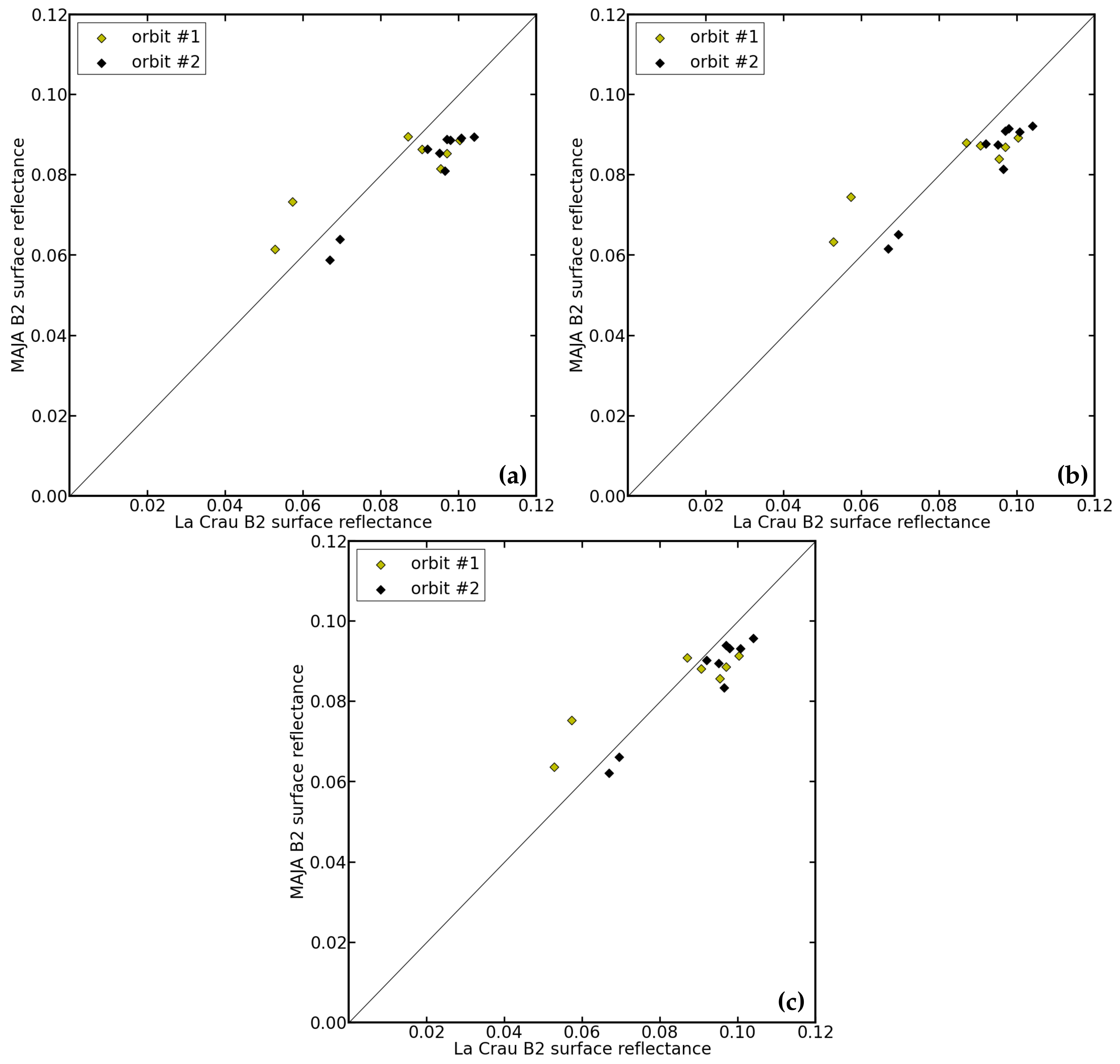
3.2.1. Validation of Surface Reflectances with La Crau Measurements

The RObotic Station for Atmosphere and Surface (ROSAS) station in La Crau (Southeast France) was set up by the Centre National d’Études Spatiales (CNES) as an automatic calibration station [47]. It is composed of a Cimel instrument mounted on a 10-m-high pole, which characterizes the atmospheric optical properties (like a regular AERONET site) but also measures the upwelling radiance over the ground to provide surface reflectance measurements. This station is part of the Radiometric Calibration Network (RadCalNet) and was designed at first to check the absolute calibration of high-resolution optical remote sensing instruments. In this study, we use the surface reflectance measurements at La Crau to validate our surface reflectance product from MAJA on the Carpentras site (presented in Section 2.4). La Crau was the only station, among the other RadCalNet stations (located in China, the United States and Namibia), to provide usable measurements over a vegetated surface. Besides, unlike the other RadCalNet stations, La Crau is the only one which measures directional surface reflectance, thus providing the bidirectional reflectance distribution function (BRDF) every 100 min. This BRDF is used to give the surface reflectance measurements in the same angular conditions as Sentinel-2A, and a temporal linear interpolation is performed to match the satellite overpass time. A continuous reflectance spectrum fit is performed on the La Crau measurements (from the native spectral bands) by a hyperspectral interpolation. Finally this reflectance spectrum is spectrally integrated to the Sentinel-2A bands.

Figure 6 assesses the performances of the surface reflectances produced by MAJA for the B2 blue band of Sentinel-2A (496 nm). The yellow and black diamonds correspond to the dates (from 1 April 2016 to 15 October 2016) of two different orbits.

Despite the observed bias, the natural temporal variability of surface reflectances is retrieved in the Sentinel-2A time series. The relative bias between MAJA and La Crau associated to this band is presented in

Table 8. Relative bias [%] of surface reflectances between the MACCS-ATCOR Joint Algorithm (MAJA) and La Crau. CAMS: Copernicus Atmosphere Monitoring Service.

	B2 (496 nm)	B3 (560 nm)	B4 (664 nm)	B8 (832 nm)	B11 (1613 nm)
constant aerosol type	−5.7	−6.6	−6.3	−7.2	−4.7
four CAMS aerosol types	−3.9	−4.6	−4.6	−6.4	−4.4
five CAMS aerosol types	−1.9	−3.1	−3.5	−5.6	−4.1

, along with the bias of the B3, B4, B8, and B11 bands.

The surface reflectances from MAJA are lower than the ones from La Crau, whatever the method used. The introduction of CAMS information (four or five aerosol types) raises the reflectances values and as a result reduces the relative bias, especially when using all CAMS aerosol types (with a relative bias reduced by 2.5 % on average over the spectral bands). However, the surface reflectances from MAJA are still lower than the observations.

The data produced by MAJA, and used in this comparison, are Level-2A products (ortho-rectified images expressed in surface reflectances). The previous level of Sentinel-2A products was Level 1C, consisting of TOA reflectances.

Table 9. Calibration coefficient (ratio of Sentinel-2A Level 1C products to La Crau top-of-atmosphere (TOA) reflectances).

	Mean Value (24 Days)	Standard Deviation
B2 (496 nm)	1.01	0.04
B3 (560 nm)	0.99	0.03
B4 (664 nm)	0.99	0.04
B8 (832 nm)	0.94	0.03
B11 (1613 nm)	0.98	0.03

checks the similarity between the Level 1C and the TOA reflectances from the La Crau station [48].

We can see that, except for the B2 band, the TOA reflectances from Sentinel-2A were already too low compared to La Crau station, with a maximum bias observed for the same band (B8) as for surface reflectance. Besides, the behaviour of the calibration coefficient in Table 9 presents the same evolution as the relative bias in Table 8, increasing with the wavelength. These similarities could partly explain the results of Table 8, even though the statistical value is limited considering only one station.

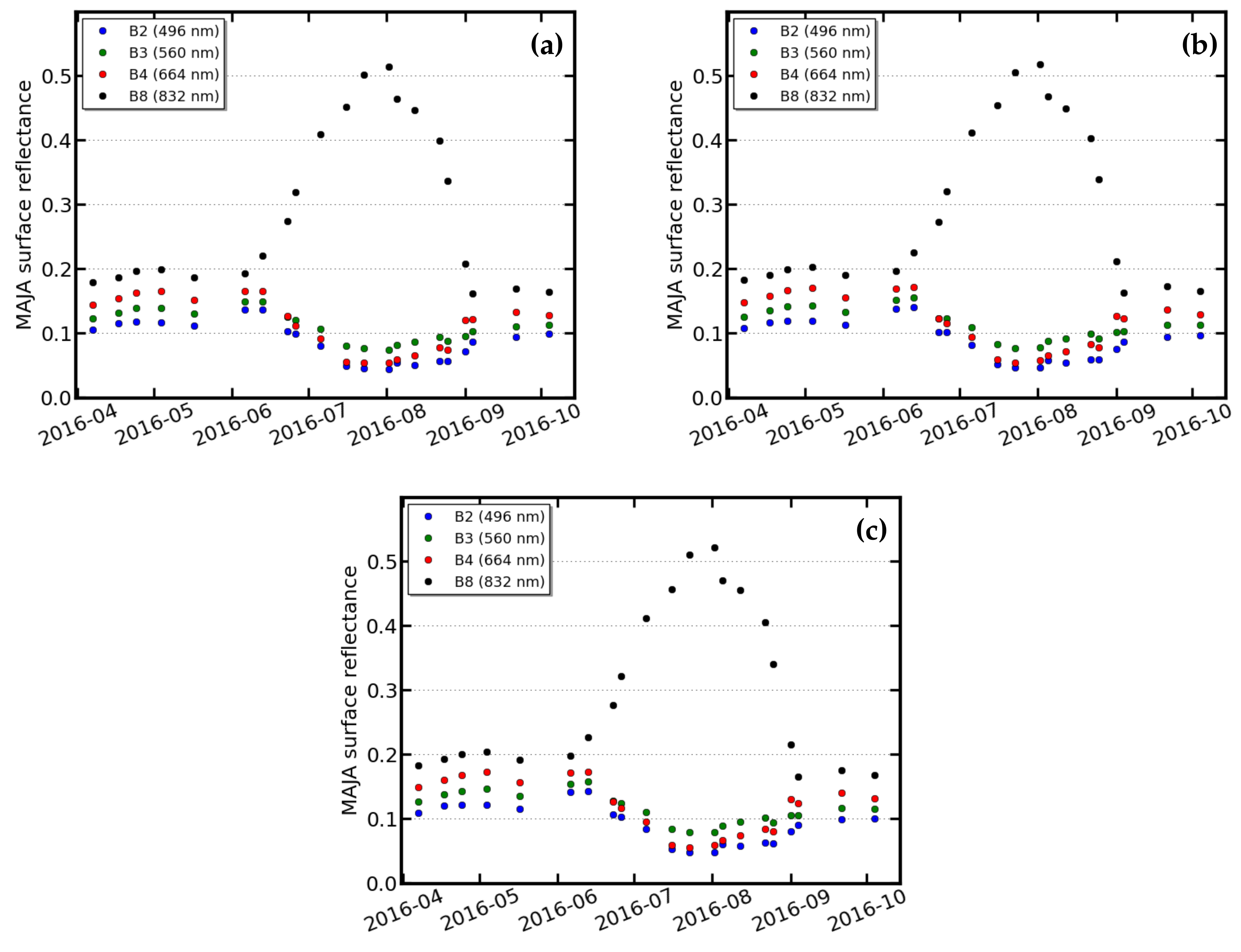
3.2.2. Smoothness of Surface Reflectances

As mentioned above, surface reflectance variation with time is expected to be smooth when observed with a sufficient repetitivity, while atmospheric effects can change quickly. This is therefore an information that can be used to compare the performances of different atmospheric correction methods. The most accurate atmospheric correction method is expected to produce smoother time series.

In this section, we try to assess the noise present in surface reflectances time series over all the validation sites presented in Table 3, to obtain a qualitative idea of the performance of the atmospheric correction. A noise criterion is set up to assess if noise has been added to or subtracted from the time series by our new correction method based on CAMS aerosol type. The time series noise criterion is defined as follows:

• A set of pixels, for which the stability will be evaluated, is chosen. One pixel every 1000 pixels along lines and columns is selected. Images are 10,980 × 10,980 pixels large, thus providing a set of 100 pixels.
• For each one of these 100 pixels, the mean surface reflectance for each date is computed within a 7 × 7 pixel neighbourhood for the spectral bands with a 10-m resolution (and a 4 × 4 pixel neighbourhood for the spectral bands with a 20-m resolution), to obtain 100 time series of surface reflectance. This size of the neighbourhood is chosen because the superposition precision of Sentinel-2A images is about 1 pixel, and registration errors of ± 2–3 pixels have been observed.
• For each one of these 100 pixels, the dates which are free from clouds, shadow, water, and snow are extracted, and the noise criterion described in [43] is computed:

  $$\sqrt{\frac{{\sum }_{i=1}^{n-2}{({\rho }_{i+1}-\frac{{\rho }_{i+2}-{\rho }_i}{d_{i+2}-d_i}(d_{i+1}-d_i)-{\rho }_i)}^2}{n-2}}$$

  (8)

  where ${\rho }_i$, ${\rho }_{i+1}$, and ${\rho }_{i+2}$ are the surface reflectances of days $d_i$, $d_{i+1}$, and $d_{i+2}$, respectively. The difference between ${\rho }_{i+1}$ and the linear interpolation of ${\rho }_i$ and ${\rho }_{i+2}$ provides a characterization of the noise of the time series. This criterion assumes a linear variation of surface reflectance within a few days, and a threshold is set up allowing a maximum of 20 days between $d_i$ and $d_{i+2}$.
• The weighted average of this criterion over the 100 pixels is computed, with the weight of each pixel being the number of dates free from clouds, shadow, water, and snow.
• Finally, the mean over the different sites presented in Section 2.4 is computed.

Before computing the noise criterion, the surface reflectances have been corrected for the directional effects, using the method from [43] and the coefficients from [44].

We compared the noise criterion obtained using CAMS with four or five aerosol types, to the value obtained using the constant aerosol type.

Table 10. Noise criterion of the MACCS-ATCOR Joint Algorithm (MAJA) surface reflectance time series, for arid sites. CAMS: Copernicus Atmosphere Monitoring Service.

	B2 (496 nm)	B3 (560 nm)	B4 (664 nm)	B8 (832 nm)	B11 (1613 nm)	B12 (2198 nm)
Constant aerosol	0.005	0.007	0.011	0.015	0.018	0.015
Four CAMS aerosol types	0.005	0.007	0.011	0.014	0.018	0.015
Five CAMS aerosol types	0.005	0.007	0.011	0.015	0.018	0.015

and

Table 11. Noise criterion of the MACCS-ATCOR Joint Algorithm (MAJA) surface reflectance time series, for vegetated sites. CAMS: Copernicus Atmosphere Monitoring Service.

	B2 (496 nm)	B3 (560 nm)	B4 (664 nm)	B8 (832 nm)	B11 (1613 nm)	B12 (2198 nm)
Constant aerosol	0.006	0.007	0.010	0.022	0.019	0.015
Four CAMS aerosol types	0.006	0.007	0.010	0.022	0.019	0.015
Five CAMS aerosol types	0.006	0.007	0.010	0.022	0.019	0.015

present the values of this noise criterion over arid and vegetated sites respectively.

For both arid and vegetated sites, the noise of the time series is not decreased when using CAMS aerosol types. In every case, except for the B8 band over arid sites, only the fourth decimal was different, but we decided not to display it as it is not significant. It seems that the gain of accuracy due to the use of a better suited aerosol type is compensated by the increase of noise due to passing from a constant aerosol to a variable aerosol type. This constant noise criterion might also partly be explained by the fact that surface reflectances calculated by MAJA tend to increase with the new methods. The average surface reflectance values are summarized in

Table 12. MAJA (MACCS-ATCOR Joint Algorithm) average surface reflectances for arid sites. CAMS: Copernicus Atmosphere Monitoring Service.

	B2 (496 nm)	B3 (560 nm)	B4 (664 nm)	B8 (832 nm)	B11 (1613 nm)	B12 (2198 nm)
constant aerosol	0.100	0.146	0.206	0.294	0.377	0.291
Four CAMS aerosol types	0.101	0.149	0.209	0.297	0.379	0.293
Five CAMS aerosol types	0.103	0.152	0.213	0.302	0.382	0.294

and

Table 13. MAJA (MACCS-ATCOR Joint Algorithm) average surface reflectances for vegetated sites. CAMS: Copernicus Atmosphere Monitoring Service.

	B2 (496 nm)	B3 (560 nm)	B4 (664 nm)	B8 (832 nm)	B11 (1613 nm)	B12 (2198 nm)
constant aerosol	0.052	0.079	0.085	0.295	0.236	0.143
Four CAMS aerosol types	0.054	0.083	0.089	0.298	0.237	0.144
Five CAMS aerosol types	0.055	0.084	0.090	0.301	0.238	0.145

. The increase of the surface reflectance values might be explained by the overall higher absorption of the CAMS aerosol types, compared to the absorption of the constant aerosol type, but this would be the subject of a future study.

In Figure 7 we focus on one pixel of the Carpentras site containing a summer crop to plot its surface reflectances time series for the blue (496 nm), green (560 nm), red (664 nm), and NIR (832 nm) spectral bands. We can observe the increase of the surface reflectance values between the method using a constant aerosol type (Figure 7a) and the methods using four (Figure 7b) and five (Figure 7c) CAMS aerosol types.

The comparisons between the noise criterion and the surface reflectances evolution could have been avoided by using a relative criterion. In this case, the noise criterion of each pixel is normalized by the pixel mean surface reflectance. This configuration has been tested but was not conclusive because, in some cases over vegetated sites, the corrected surface reflectances can be very close to zero (as low as 0.01). The relative criterion normalized by this close to zero value then presented extravagant values over some sites. This is the reason why the absolute criterion was kept, rather than the relative criterion.

Finally, the new version of MAJA does not bring an overall decrease of the noise in surface reflectances, which might be related to the increase in the average reflectances and to passing from a constant aerosol to a variable aerosol type.

4. Conclusions

The products from the Copernicus Atmosphere Monitoring Service (CAMS) were introduced in the atmospheric correction of Sentinel-2A time series by the MACCS-ATCOR Joint Algorithm (MAJA) software. Before this study, MAJA estimated aerosol optical thickness using a constant aerosol type. The study presented in this paper takes advantage of the aerosol optical thickness (AOT) forecasts from the CAMS system for five different aerosol types to select a variable aerosol type for the atmospheric correction. A weighted interpolation of these types is performed using the respective AOT predictions from CAMS to estimate the AOT present on the image.

Several validation methods were used to assess the performances of this new configuration. Firstly, we compared the AOT estimated by MAJA to the ground-based observations from the Aerosol Robotic Network (AERONET). Various sites where AERONET data are available were selected to represent both arid and vegetated sites and a large variability of surface and aerosol conditions. Using CAMS aerosol type within MAJA processing led to a significant improvement of AOT estimation over arid sites with an RMSE reduced by 28% (from 0.095 to 0.068). Conversely, the performances slightly deteriorated over vegetated sites with the RMSE increasing by 13% from 0.054 to 0.061.

Secondly, we validated the surface reflectances produced by MAJA. To do so, a comparison was made with the ground-based reflectance measurements from the La Crau station. Using CAMS data led to a decrease of the relative bias which was observed with the constant model, by 2.5 % on average over the spectral bands.

Finally, a noise criterion was defined to evaluate if the new method using CAMS was adding noise to the surface reflectance time series. The results showed no improvement of this criterion over the spectral bands and the validation sites.

Globally, our results show a significant improvement of the AOT estimates over arid sites, a reduction of a bias observed on surface reflectances of the La Crau site, and nearly no change in the smoothness of surface reflectances. The method proposed in this paper (i.e., using CAMS products) presents several advantages from an operational point of view. The manual definition of a global map of aerosol types is avoided, and a variation with time of the aerosol type is made possible. This introduction of ancillary data does not overly complicate the whole system, because CAMS data is freely and easily available in time through the European Centre for Medium-Range Weather Forecasts (ECMWF). The method proposed in this study will soon be implemented in version 3.0 of MAJA.

Different improvements could be made in the future. The CAMS system is relatively new, indicating potential evolutions in the way the aerosol forecasts are processed. The optical properties of the different aerosol types will also be subject to future changes, leading to potentially more accurate predictions which should enhance the performances within MAJA.

The total aerosol optical thickness predicted by CAMS could also be used directly, instead of the AOT estimated by MAJA, when it is not possible to make an accurate estimation, for instance when too many pixels are marked as cloud, shadow, snow or water.

Finally, the recent launch of the Sentinel-2B satellite on 7 March 2017 will bring a better repetitiveness of all Earth’s land surface observations, improving the performances of the multi-temporal method included in MAJA.

References

1. Fraser, R.S.; Kaufman, Y.J. The relative importance of aerosol scattering and absorption in remote sensing. IEEE Trans. Geosci. Remote Sens. 1985, 5, 625–633. [Google Scholar] [CrossRef]
2. Vermote, E.; Tanré, D.; Deuzé, J.; Herman, M.; Morcette, J.J. Second Simulation of the Satellite Signal in the Solar Spectrum, 6S: An overview. IEEE Trans. Geosci. Remote Sens. 1997, 35, 675–686. [Google Scholar] [CrossRef]
3. Kaufman, Y.J.; Sendra, C. Algorithm for automatic atmospheric corrections to visible and near-IR satellite imagery. Int. J. Remote Sens. 1988, 9, 1357–1381. [Google Scholar] [CrossRef]
4. Liang, S.; Fang, H.; Chen, M. Atmospheric correction of Landsat ETM+ land surface imagery. I. Methods. IEEE Trans. Geosci. Remote Sens. 2001, 39, 2490–2498. [Google Scholar] [CrossRef]
5. Ouaidrari, H.; Vermote, E.F. Operational atmospheric correction of Landsat TM data. Remote Sens. Environ. 1999, 70, 4–15. [Google Scholar] [CrossRef]
6. Ju, J.; Roy, D.P.; Vermote, E.; Masek, J.; Kovalskyy, V. Continental-scale validation of MODIS-based and LEDAPS Landsat ETM+ atmospheric correction methods. Remote Sens. Environ. 2012, 122, 175–184. [Google Scholar] [CrossRef]
7. Richter, R. A spatially adaptive fast atmospheric correction algorithm. Int. J. Remote Sens. 1996, 17, 1201–1214. [Google Scholar] [CrossRef]
8. Richter, R.; Schläpfer, D.; Müller, A. An automatic atmospheric correction algorithm for visible/NIR imagery. Int. J. Remote Sens. 2006, 27, 2077–2085. [Google Scholar] [CrossRef]
9. Vermote, E.; Justice, C.; Claverie, M.; Franch, B. Preliminary analysis of the performance of the Landsat 8/ OLI land surface reflectance product. Remote Sens. Environ. 2016, 185, 46–56. [Google Scholar] [CrossRef]
10. Hagolle, O.; Huc, M.; Villa Pascual, D.; Dedieu, G. A multi-temporal and multi-spectral method to estimate aerosol optical thickness over land, for the atmospheric correction of FORMOSAT-2, LANDSAT, VENμS and SENTINEL-2 images. Remote Sens. 2015, 7, 2668–2691. [Google Scholar] [CrossRef]
11. Rahman, H.; Dedieu, G. SMAC: A simplified method for the atmospheric correction of satellite measurements in the solar spectrum. Int. J. Remote Sens. 1994, 15, 123–143. [Google Scholar] [CrossRef]
12. Hagolle, O.; Dedieu, G.; Mougenot, B.; Debaecker, V.; Duchemin, B.; Meygret, A. Correction of aerosol effects on multi-temporal images acquired with constant viewing angles: Application to Formosat-2 images. Remote Sens. Environ. 2008, 112, 1689–1701. [Google Scholar] [CrossRef] [Green Version]
13. Levy, R.C.; Mattoo, S.; Munchak, L.A.; Remer, L.A.; Sayer, A.M.; Patadia, F.; Hsu, N.C. The Collection 6 MODIS aerosol products over land and ocean. Atmos. Meas. Tech. 2013, 6, 2989–3034. [Google Scholar] [CrossRef]
14. Remer, L.A.; Kaufman, Y.J.; Tanré, D.; Mattoo, S.; Chu, D.A.; Martins, J.V.; Li, R.R.; Ichoku, C.; Levy, R.C.; Kleidman, R.G. The MODIS aerosol algorithm, products, and validation. J. Atmos. Sci. 2005, 62, 947–973. [Google Scholar] [CrossRef]
15. Lenoble, J.; Herman, M.; Deuzé, J.L.; Lafrance, B.; Santer, R.; Tanré, D. A successive order of scattering code for solving the vector equation of transfer in the Earth’s atmosphere with aerosols. J. Quant. Spectrosc. Radiat. Transf. 2007, 107, 479–507. [Google Scholar] [CrossRef]
16. Dubovik, O.; Holben, B.; Eck, T.F.; Smirnov, A.; Kaufman, Y.J.; King, M.D.; Tanré, D.; Slutsker, I. Variability of absorption and optical properties of key aerosol types observed in worldwide locations. J. Atmos. Sci. 2002, 59, 590–608. [Google Scholar] [CrossRef]
17. Colarco, P.; da Silva, A.; Chin, M.; Diehl, T. Online simulations of global aerosol distributions in the NASA GEOS-4 model and comparisons to satellite and ground-based aerosol optical depth. J. Geophys. Res. 2010, 115. [Google Scholar] [CrossRef]
18. Lu, S.; Huang, H.-C.; Hou, Y.-T.; Tang, Y.; McQueen, J.; da Silva, A.; Chin, M.; Joseph, E.; Stockwell, W. Development of NCEP Global Aerosol Forecasting System: An Overview and Its application for improving weather and air quality forecasts. In NATO Science for Peace and Security Series: Air Pollution Modelling and Its Application XX; Steyn, D.G., Rao, S.T., Eds.; Springer Publications: Dordrecht, The Netherlands, 2010. [Google Scholar]
19. Chin, M.; Rood, R.B.; Lin, S.-J.; Müller, J.-F.; Thompson, A.M. Atmospheric sulfur cycle simulated in the global model GOCART: Model description and global properties. J. Geophys. Res. 2000, 105, 24671–24687. [Google Scholar] [CrossRef]
20. Yu, P.; Toon, O.B.; Bardeen, C.G.; Mills, M.J.; Fan, T.; English, J.M.; Neely, R.R. Evaluations of tropospheric aerosol properties simulated by the community earth system model with a sectional aerosol microphysics scheme. J. Adv. Model. Earth Syst. 2015, 7, 865–914. [Google Scholar] [CrossRef] [PubMed] [Green Version]
21. Rubin, J.I.; Reid, J.S.; Hansen, J.A.; Anderson, J.L.; Collins, N.; Hoar, T.J.; Hogan, T.; Lynch, P.; McLay, J.; Reynolds, C.A.; et al. Development of the Ensemble Navy Aerosol Analysis Prediction System (ENAAPS) and its application of the Data Assimilation Research Testbed (DART) in support of aerosol forecasting. Atmos. Chem. Phys. 2016, 16, 3927–3951. [Google Scholar] [CrossRef]
22. Toon, O.B.; Turco, R.P.; Westphal, D.; Malone, R.; Liu, M.S. A Multidimensional Model for Aerosols: Description of Computational Analogs. J. Atmos. Sci. 1988, 45, 2123–2144. [Google Scholar] [CrossRef]
23. Christensen, J.H. The Danish eulerian hemispheric model—A three-dimensional air pollution model used for the arctic. Atmos. Environ. 1997, 31, 4169–4191. [Google Scholar] [CrossRef]
24. Witek, M.L.; Flatau, P.J.; Quinn, P.K.; Westphal, D.L. Global sea-salt modeling: Results and validation against multicampaign shipboard measurements. J. Geophys. Res. 2007, 112. [Google Scholar] [CrossRef]
25. Reid, J.S.; Hyer, E.J.; Prins, E.M.; Westphal, D.L.; Zhang, J.; Wang, J.; Christopher, S.A.; Curtis, C.A.; Schmidt, C.C.; Eleuterio, D.P.; et al. Global Monitoring and Forecasting of Biomass-Burning Smoke: Description of and Lessons From the Fire Locating and Modeling of Burning Emissions (FLAMBE) Program. IEEE J. Sel. Top. Appl. Earth Obs. Remote Sens. 2009, 2, 144–162. [Google Scholar] [CrossRef]
26. Morcrette, J.J.; Boucher, O.; Jones, L.; Salmond, D.; Bechtold, P.; Beljaars, A.; Benedetti, A.; Bonet, A.; Kaiser, J.W.; Razinger, M.; et al. Aerosol analysis and forecast in the European center for medium-range weather forecasts integrated forecast system: forward modeling. J. Geophys. Res. 2009, 114. [Google Scholar] [CrossRef]
27. Benedetti, A.; Morcrette, J.J.; Boucher, O.; Dethof, A.; Engelen, R.; Fisher, M.; Flentje, H.; Huneeus, N.; Jones, L.; Kaiser, J.; et al. Aerosol analysis and forecast in the European center for medium-range weather forecasts integrated forecast system: 2. Data assimilation. J. Geophys. Res. 2009, 114. [Google Scholar] [CrossRef]
28. van der Werf, G.R.; Randerson, J.T.; Giglio, L.; Collatz, G.J.; Kasibhatla, P.S.; Arellano, A.F. Interannual variability in global biomass burning emissions from 1997 to 2004. Atmos. Chem. Phys. 2006, 6, 3423–3441. [Google Scholar] [CrossRef] [Green Version]
29. Van der Werf, G.R.; Randerson, J.T.; Giglio, L.; Collatz, G.J.; Mu, M.; Kasibhatla, P.S.; Morton, D.C.; DeFries, R.S.; Jin, Y.; van Leeuwen, T.T. Global fire emissions and the contribution of deforestation, savanna, forest, agricultural, and peat fires (1997–2009). Atmos. Chem. Phys. 2010, 10, 11707–11735. [Google Scholar] [CrossRef] [Green Version]
30. Bond, T.C.; Streets, D.G.; Yarber, K.F.; Nelson, S.M.; Woo, J.H.; Klimont, Z. A technology-based global inventory of black and organic carbon emissions from combustion. J. Geophys. Res. 2004, 109. [Google Scholar] [CrossRef]
31. Janssens-Maenhout, G.; Dentener, F.; van Aardenne, J.; Monni, S.; Pagliari, V.; Orlandini, L.; Klimont, Z.; Kurokawa, J.I.; Akimoto, H.; Ohara, T.; et al. EDGAR-HTAP: A Harmonized Gridded Air Pollution Emission Dataset Based on National Inventories. Available online: http://edgar.jrc.ec.europa.eu/htap/EDGAR-HTAP_v1_final_jan2012.pdf (accessed on 8 November 2017).
32. Eskes, H.J.; Antonakaki, T.; Basart, S.; Benedictow, A.; Blechschmidt, A.-M.; Chabrillat, S.; Christophe, Y.; Clark, H.; Cuevas, E.; Hansen, K.M.; et al. Upgrade verification note for the CAMS near-real time global atmospheric composition service, Copernicus Atmosphere Monitoring Service (CAMS) Report. Available online: http://atmosphere.copernicus.eu/sites/default/files/repository/CAMS84_2015SC1_D84.3.2_201611_esuite_v1_0.pdf (accessed on 8 November 2017).
33. Drusch, M.; del Bello, U.; Carlier, S.; Colin, O.; Fernandez, V.; Gascon, F.; Hoersch, B.; Isola, C.; Laberinti, P.; Martimort, P.; et al. Sentinel-2: ESA’s optical high-resolution mission for GMES operational services. Remote Sens. Environ. 2012, 120, 25–36. [Google Scholar] [CrossRef]
34. Holben, B.N.; Eck, T.F.; Slutsker, I.; Tanré, D.; Buis, J.P.; Setzer, A.; Vermote, E.; Reagan, J.A.; Kaufman, Y.J.; Nakajima, T.; et al. AERONET—A federated instrument network and data archive for aerosol characterization. Remote Sens. Environ. 1998, 66, 1–16. [Google Scholar] [CrossRef]
35. Dubovik, O.; Smirnov, A.; Holben, B.N.; King, M.D.; Kaufman, Y.J.; Eck, T.F.; Slutsker, I. Accuracy assessments of aerosol optical properties retrieved from Aerosol Robotic Network (AERONET) Sun and sky radiance measurements. J. Geophys. Res. 2000, 105, 9791–9806. [Google Scholar] [CrossRef]
36. Reddy, M.S.; Boucher, O.; Bellouin, N.; Schulz, M.; Balkanski, Y.; Dufresne, J.-L.; Pham, M. Estimates of global multicomponent aerosol optical depth and direct radiative perturbation in the Laboratoire de Météorologie Dynamique general circulation model. J. Geophys. Res. 2005, 110. [Google Scholar] [CrossRef] [Green Version]
37. Toon, O.B.; Ackerman, T.P. Algorithms for the calculation of scattering by stratified spheres. Appl. Opt. 1981, 20, 3657–3660. [Google Scholar] [CrossRef] [PubMed]
38. Stephens, G.L. Optical Properties of Eight Water Cloud Types; CSIRO: Melbourne, Australia, 1979. [Google Scholar]
39. Mishchenko, M.I.; Lacis, A.A.; Carlson, B.E.; Travis, L.D. Nonsphericity of dust-like tropospheric aerosols: Implications for aerosol remote sensing and climate modeling. Geophys. Res. Lett. 1995, 22, 1077–1080. [Google Scholar] [CrossRef]
40. Fu, Q.; Thorsen, T.J.; Su, J.; Ge, J.M.; Huang, J.P. Test of Mie-based single-scattering properties of non-spherical dust aerosols in radiative flux calculations. J. Quant. Spectrosc. Radiat. Transf. 2009, 110, 1640–1653. [Google Scholar] [CrossRef]
41. Mishchenko, M.I.; Travis, L.D.; Mackowski, D.W. T-Matrix computations of light scattering by nonspherical particles: A review. J. Quant. Spectrosc. Radiat. Transf. 1996, 55, 535–575. [Google Scholar] [CrossRef]
42. Tang, I.N. Thermodynamic and optical properties of mixed-salt aerosols of atmospheric importance. J. Geophys. Res. 1997, 102, 1883–1893. [Google Scholar] [CrossRef]
43. Vermote, E.; Justice, C.O.; Bréon, F.-M. Towards a generalized approach for correction of the BRDF effect in MODIS directional reflectances. IEEE Trans. Geosci. Remote Sens. 2009, 47, 898–908. [Google Scholar] [CrossRef]
44. Roy, D.P.; Zhang, H.K.; Ju, J.; Gomez-Dans, J.L.; Lewis, P.E.; Schaaf, C.B.; Sun, Q.; Li, J.; Huang, H.; Kovalskyy, V. A general method to normalize Landsat reflectance data to nadir BRDF adjusted reflectance. Remote Sens. Environ. 2016, 176, 255–271. [Google Scholar] [CrossRef]
45. Smirnov, A.; Holben, B.N.; Eck, T.F.; Dubovik, O.; Slutsker, I. Cloud-Screening and quality control algorithms for the AERONET database. Remote Sens. Environ. 2000, 73, 337–349. [Google Scholar] [CrossRef]
46. Woodward, S. Modeling the atmospheric life cycle and radiative impact of mineral dust in the Hadley Centre climate model. J. Geophys. Res. 2001, 106, 18155–18166. [Google Scholar] [CrossRef]
47. Meygret, A.; Santer, R.P.; Berthelot, B. ROSAS: A robotic station for atmosphere and surface characterization dedicated to on-orbit calibration. In Proceedings of the SPIE The International Society for Optical Engineering, Earth Observing Systems XVI, San Diego, CA, USA, 21 August 2011. [Google Scholar]
48. Meygret, A.; Marcq, S.; Besson, B.; Guilleminot, N.; Desjardins, C. ROSAS status. In Proceedings of the CEOS RadCalNet meeting, Beijing, China, 18 July 2016. [Google Scholar]
Figure 1. Copernicus Atmosphere Monitoring Service (CAMS) aerosol optical thickness forecasts at 550 nm on 14 June 2016, 03:00 UTC (Coordinated Universal Time): (a) Dust, (b) Sea Salt, (c) Black Carbon, and (d) Sulfate. AOT: aerosol optical thickness.
Remotesensing 09 01230 g001
Figure 2. Location of validation sites.
Remotesensing 09 01230 g002
Figure 3. Scatter plots of aerosol optical thickness (AOT) at 550 nm versus AERONET (Aerosol Robotic Network) observations over arid sites: (a) AOT predicted by CAMS (Copernicus Atmosphere Monitoring Service); (b) AOT estimated by the MACCS-ATCOR Joint Algorithm (MAJA) with a constant aerosol type; (c) AOT estimated by MAJA using four CAMS aerosol types; and (d) AOT estimated by MAJA using five CAMS aerosol types. RMSE: root-mean-square error. std: standard deviation.
Remotesensing 09 01230 g003
Figure 4. Scatter plots of aerosol optical thickness (AOT) at 550 nm versus AERONET (Aerosol Robotic Network) observations over vegetated sites: (a) AOT predicted by CAMS (Copernicus Atmosphere Monitoring Service); (b) AOT estimated by the MACCS-ATCOR Joint Algorithm (MAJA) with a constant aerosol type; (c) AOT estimated by MAJA using four CAMS aerosol types; and (d) AOT estimated by MAJA using five CAMS aerosol types. RMSE: root-mean-square error. std: standard deviation.
Remotesensing 09 01230 g004
Figure 5. Ouarzazate (Morocco) on 6 June 2016: (a) estimated aerosol optical thickness (AOT) at 550 nm; (b) surface reflectance after atmospheric correction using the constant aerosol type; (c) estimated AOT at 550 nm; and (d) surface reflectance after atmospheric correction using five CAMS (Copernicus Atmosphere Monitoring Service) aerosol types. For the AOT in (a,c), clouds are in dark red, their shadows are in black, water is in blue, and snow in bright red. For the surface reflectance in (b,d) clouds are circled in green, their shadows in yellow, water is circled in blue, and snow is in pink.
Remotesensing 09 01230 g005
Figure 6. For the B2 band (496 nm), surface reflectances calculated by the MACCS-ATCOR Joint Algorithm (MAJA) as a function of La Crau observations: (a) with a constant aerosol type; (b) with four CAMS (Copernicus Atmosphere Monitoring Service) aerosol types; and (c) with five CAMS aerosol types.
Remotesensing 09 01230 g006
Figure 7. MAJA (MACCS-ATCOR Joint Algorithm) surface reflectance time series over a summer crop pixel from the Carpentras site: (a) with a constant aerosol type; (b) with four CAMS (Copernicus Atmosphere Monitoring Service) aerosol types; and (c) with five CAMS aerosol types.
Remotesensing 09 01230 g007