Change Detection Using High Resolution Remote Sensing Images Based on Active Learning and Markov Random Fields

Abstract

Change detection has been widely used in remote sensing, such as for disaster assessment and urban expansion detection. Although it is convenient to use unsupervised methods to detect changes from multi-temporal images, the results could be further improved. In supervised methods, heavy data labelling tasks are needed, and the sample annotation process with real categories is tedious and costly. To relieve the burden of labelling and to obtain satisfactory results, we propose an interactive change detection framework based on active learning and Markov random field (MRF). More specifically, a limited number of representative objects are found in an unsupervised way at the beginning. Then, the very limited samples are labelled as “change” or “no change” to train a simple binary classification model, i.e., a Gaussian process model. By using this model, we then select and label the most informative samples by “the easiest” sample selection strategy to update the former weak classification model until the detection results do not change notably. Finally, the maximum a posteriori (MAP) change detection is efficiently computed via the min-cut-based integer optimization algorithm. The time consuming and laborious manual labelling process can be reduced substantially, and a desirable detection result can be obtained. The experiments on several WorldView-2 images demonstrate the effectiveness of the proposed method.

1. Introduction

Change detection is the process to find inconsistent regions in different temporal images of the same area [1]. Recently, high resolution remote sensing (HRRS) images have become the major sources for change detection studies. The change detection technique is widely used in monitoring landscape conditions [2], the influence of natural disasters [3] and urban expansion, discovering the vegetation changes, assessing desertification [4] and detecting other urban or natural environmental changes [5,6,7]. In the past decades, numerous change detection methods have been developed and considerable studies have addressed the automatic and accurate detection of changes from multi-temporal images. The most general change detection framework in remote sensing comprises of feature extraction and decision making. At the feature level, some methods focus on the completeness of color, texture and structural information [8,9], while others intend to use object-based analysis and MRF to emphasis spatial information [10,11,12]. At the decision level, most of these methods can be categorized into supervised, semi-supervised and unsupervised methods [13,14]. Supervised and semi-supervised methods obtain the change messages by learning from labelled samples, while unsupervised methods detect changes appearing in the observed region by comparing the distribution of pixel values. As an application-oriented research, change detection is a complicated process and is attracting more and more attention.

Supervised change detection methods sometimes detect land cover changes from classification results [15]. If multitemporal ground truth information is available, supervised techniques can be applied. The ground truth is used to train classification models. Post-classification comparison techniques obtain the change message from multiple classification maps of different temporal images to detect category transitions [16,17]. Based on the set of reliable labelling samples, the supervised methods can obtain good performance and specific category transition. Molina et al. [18] proposed to use a parametric multi-sensor Bayesian data fusion approach and a Support Vector Machine (SVM) for change detection problems. Wu et al. [19] explored a scene change detection framework for HRRS images, with a bag-of-visual-words (BOVW) model and classification-based methods [20]. Then, post-classification and compound classification were evaluated for their performances in the “from–to” change results. Nevertheless, whether or not the corresponding samples in the experimental dataset are correctly classified, some misclassified samples may result in errors on the post-classification change detection map. Almost all classifiers are sensitive to noise. Besides, preparing training samples for supervised classifiers is a complex, time consuming and expensive process. To avoid the bad effects of misclassified samples and consider the temporal correlation, some supervised methods stack multi-temporal images together and take into account the dependence between two images of the same area [21,22]. The general idea is to characterize pixels or objects by stacking the feature vectors of two images. Then, land-cover transition classifiers are carried out to recognize specific transitions provided by training samples. In [22], Volpi et al. adopted the nonlinear SVMs to cope with the high intra-class variability, which achieved high detection accuracy in very high geometrical resolution images. In addition, to reduce the tedious workload of labelling, some semi-supervised change detection methods are proposed. Shao et al. [23] proposed a novel and robust semi-supervised fuzzy C-means clustering algorithm to analyze the difference image. Chen et al. [24] proposed a semisupervised context-sensitive method by analyzing the posterior of probabilistic Gaussian process classifier within an MRF model. An et al. [25] proposed a novel semi-supervised SAR images change detection methods using random fields based on maximum entropy principle. The proposed model takes full advantages of the image information from both the labelled and the unlabelled samples, providing appropriate detection results even using a small number of labelled samples. All the aforementioned supervised and semi-supervised methods based on classification are intrinsically suitable to detect changes in multisensor/multisource data.

If no ground truth is available, unsupervised methods can be adopted. Unsupervised change detection methods detect land cover change based on the property of data, mainly referring to the difference image. Difference image-based unsupervised change detection mainly includes two pivotal steps: producing a difference image and analyzing the difference image to identify the pixels as changed or unchanged. The first step is to compare two co-registered multi-temporal images to create the difference image, in which different mathematical operators can be used (e.g., image differencing, image rationing, spectral gradient differencing, and change vector analysis). The second step is to separate the pixels of difference image into changed or unchanged classes to obtain the change detection map. Nielsen [26] proposed the iteratively reweighted multivariate alteration detection (IR-MAD) method for change detection, which established the technique of canonical correlation analysis. Then, Marpu et al. [27] improved the IR-MAD method by the usage of an initial change mask to eliminate strong changes. Liu et al. [28] proposed a hierarchical scheme by considering spectral change information to identify the change classes. Considering reference samples are often not available in real applications, the proposed approach is designed in an unsupervised way. To detect changes in the increasing amount of available HRRS imagery, Leichtle et al. [11] proposed an object-based approach using principal component analysis (PCA) and k-means clustering for the discrimination of changed and unchanged buildings. Byun et al. [29] introduced a novel unsupervised change detection approach based on image fusion. Shah-Hosseini et al. [30] proposed two automatic kernel-based change detection algorithms based on kernel clustering and support vector data description algorithms in high dimensional Hilbert space. Sinha et al. [31] proposed a rank-based metric selection process through computation of four difference-based indices using a Max–Min/Max normalization approach. Although these unsupervised methods do not need tedious and expensive annotations, certain objective factors such as the atmosphere conditions, sensor calibration, etc., can affect the derived difference image. Moreover, choosing an appropriate threshold to detect change areas is also a very difficult task. Most importantly, the change detection results of unsupervised methods are often unsatisfactory compared with supervised methods.

Considering many change detection methods only utilize the attribute information (color and texture), we further exploit the fact that, in detecting real-world changes, it is very likely that changes occur in a relatively large area, which means the spatially neighboring pixels belong to the same class (change or no change) [14]. This prior, which can be modeled as MRFs, encourages piecewise smooth change detection and eliminates the “superpixel-noises” of active learning results. In either supervised and unsupervised methods, the integration of spatial and attribute information can significantly improve the detection results. To combine spectral and spatial information, Zhu et al. [32] proposed to formulate saliency detection as a maximum a posteriori (MAP) probability estimation problem, which could find the salient regions from the background through MRF learning. In [33], the authors used multitask joint sparse representation and a stepwise MRF framework to effectively handle high data correlation and the spatial coherency. In [34], Li et al. integrated the subspace multinomial logistic regression methods with the multilevel logistic Markov-Gibbs MRF, providing accurate characterization of hyperspectral imagery in both the spectral and the spatial domain. For change detection objective, Yousif et al. [12] proposed the iterated conditional models framework to characterize the relationship between pixels’ class-labels in a nonlocal scale, which effectively preserved spatial details and reduced speckle effects in multi-temporal SAR images. These methods formulate the spatial constraints into MRF model, providing superior performance compared with results when only using attribute information.

As mentioned above, it is a difficult task to construct the large training sample set for supervised methods, which may need extensive field investigations. However, whether a region has changed could be uncertain without human intervention for unsupervised methods. In this paper, our goal is to use the minimum labelling samples to obtain the most reliable change detection results. To reduce the workload of manual annotation, an active learning framework is proposed to improve the effectiveness of limited labelled training data. Active learning can label massive unlabelled instances with minimal cost by selecting the most informative samples from all unlabelled datasets. Then, more accurate change detection can be established with those informative samples. To further improve the detection results, the contextual information is used as spatial constraints to generate MRFs. More specifically, we firstly utilize a superpixel segmentation method, i.e., SLIC algorithm [35], to over-segment one image and use it as a segmentation mask to be applied on another image for the corresponding objects. Then, we extract color and texture features to measure the similarity of corresponding superpixels using the histogram intersection kernel. Based on the feature similarity, we can find a limited number of the most representative superpixels by an unsupervised method, e.g., k-means clustering, and then manually annotate these representative superpixels with “change” or “no change” labels. Next, we can use these samples to train a weak binary classification model, i.e., a Gaussian process model. By using this model, we then select the most informative samples from the unlabelled dataset and manually label them to update the former weak classification model. After a few iterations, we can get a good classification model based on the informative training sample set. Finally, the classification results of pixels are formulated in MRFs. The final change labels from a posterior distribution are built on the active learning classifiers and on a spatial MRFs prior of the change labels.

Although there are many image classification methods using active learning, very few of them directly apply active learning in change detection problems. This study presents an interactive change detection system with active learning and MRFs. The main contributions of this paper are as follows:

• An interactive object-based change detection framework is proposed, which uses active learning with Gaussian processes to update the change detection results iteratively. After the comprehensive analysis of the sample selection strategy in change detection, a new sample selection method is introduced by choosing the easiest one from several candidate samples with the consideration of the representativeness and the convenience of labelling.
• The integration of attribute information (including color and texture) and contextual information. The contextual information is introduced to remove the “superpixel-noise” in the detection results of active learning. It is formulated as MRFs and can be efficiently solved by the min-cut-based integer optimization algorithm.

This paper is organized as follows. In Section 2, we briefly review the background about active learning, Gaussian processes and MRFs. In Section 3, we describe the interactive change detection framework using active learning and MRFs in detail. In Section 4, the experimental results on multiple datasets are presented to show the performance of the proposed method. Finally, the conclusion is drawn in Section 5.

2. Background

In this section, the outline of the active learning and Gaussian processes are presented. In addition, the MRF is introduced to integrate the contextual information and attribute information.

2.1. Active Learning

The problem of labelling massive samples in real-world applications with minimal cost has been paid considerable attention in recent years, especially in deep learning and big data areas. It is a difficult task to label different classes of training data in supervised methods, but manual annotation is necessary when the system needs to detect specific categories. Thus, active learning [36] was proposed to select limited training samples and to train the classifiers in machine learning. It is known that a classifier trained on a small set of well-chosen examples can perform as well as a classifier trained on more randomly chosen examples, and the computational complexity is also significantly reduced [37,38,39]. The main task of active learning is to automatically select the most informative and representative instances to efficiently reduce the labelling workload. In most cases, to ensure the completeness of training sets and a good performance in the classification, massive labelling often results in redundant labelled samples. Finding the most informative samples in abundant unlabelled data is the key issue in active learning.

Active learning generally consists of two components [40]: training and query. On the given labelled dataset, the training algorithm usually maintains a series of standard classifiers. The query algorithm tries to select the most informative samples from unlabelled dataset, then the selected samples will be labelled by supervisors and be added into the training sets. After that, the training algorithm obtains a new classifier based on the updated training set. After a number of iterations, the performance of the classifier will be improved. Suppose we have a training set $\mathbf{X}$ composed by m labelled examples $\mathbf{X}=\{{\mathbf{x}}_{\mathbf{1}},{\mathbf{x}}_{\mathbf{2}},\dots ,{\mathbf{x}}_{\mathbf{m}}\}({\mathbf{x}}_{\mathbf{i}}\in R^d)$ with corresponding labels $\mathbf{y}={\{y_1,y_2,\dots ,y_m\}}^T(y_i\in \{\pm 1\})$. In active learning, the most informative samples are selected from unlabelled dataset $\mathbf{U}=\{{\mathbf{u}}_{\mathbf{1}},{\mathbf{u}}_{\mathbf{2}},\dots ,{\mathbf{u}}_{\mathbf{n}}\}(n\gg m)$, where n is the number of unlabelled samples.

There are two main frameworks of active learning [39]: stream-based selective sampling and pool-based selective sampling, which are based on the different data evaluation methods of the unlabelled data. Stream-based sampling needs to set a minimum threshold on the informative evaluation of the unlabelled instances. The instances exceeding this threshold will be queried and labelled. However, the threshold varies for different circumstances, and this method is inapplicable to some cases. For the pool-based selective sampling, some specific criteria are used to sort and query the most informative instances from the pool of unlabelled instances. The pool-based sampling is widely studied and used for many real-world applications in machine learning [41,42,43].

2.2. Gaussian Processes

As for supervised learning, classification uncertainties can be estimated in a Bayesian manner directly with Gaussian processes [44]. A Gaussian process is a stochastic process specified by its mean and covariance function. However, it is difficult to solve large-scale classification problems with high computational complexity using Gaussian processes. In 2012, Freytag et al. [45] put forward the optimization calculation methods for Gaussian processes, which allows estimating these uncertainties with linear or even constant time with respect to the number of training examples.

Given examples $\mathbf{X}$ and the corresponding labels $\mathbf{y}$, we try to estimate the underlying latent function f which maps inputs $\mathbf{X}$ to outputs $\mathbf{y}$. We assume that outputs $y_i$ are disturbed by Gaussian noise $ϵ\sim N(0,{\sigma }^2),\sigma$ is the standard deviation of white noise, i.e., $y_i=f({\mathbf{x}}_{\mathbf{i}})+ϵ,y_i$ is the predictive value for testing sample and the symbol of $y_i$ reflects the category of that sample, ${\mathbf{x}}_{\mathbf{i}}$ is the descriptor vector for that sample. The Gaussian process uses a non-parameterized Bayesian formulation to solve this problem. Assuming the latent function f is sampled from a Gaussian process with zero mean and covariance (kernel) function $\mathbf{K}$, the output $y_{*}$ for a new test input ${\mathbf{x}}_{*}$, which is actually the predicted mean value ${\mu }_{*}({\mathbf{x}}_{*})$, can be directly obtained from the predictive distribution [45]:

$$\begin{array}{ccc}\hfill {\mu }_{*}({\mathbf{x}}_{*})& =& k_{*}^T{(\mathbf{K}+{\sigma }^2\mathbf{I})}^{-1}y,\hfill \end{array}$$

(1)

$$\begin{array}{ccc}\hfill {\sigma }_{*}^2({\mathbf{x}}_{*})& =& k_{**}+{\sigma }^2-k_{*}^T{(\mathbf{K}+{\sigma }^2\mathbf{I})}^{-1}{k}_{*},\hfill \end{array}$$

(2)

where ${\mathbf{x}}_{*}$ is the descriptor vector for a new test input, y is a vector containing the label values of the training set, $k_{*},k_{**}$ and $\mathbf{K}$ are the kernel values of the test input, between training set and test input, and of the training set itself, respectively. For two input vectors, $\mathbf{x},{\mathbf{x}}^{\prime }\in R^d$, the kernel values of $k_{*},k_{**}$ and $\mathbf{K}$ are computed used the histogram intersection kernel (HIK),

$${\mathbf{K}}^{hik}(\mathbf{x},{\mathbf{x}}^{\prime })=\sum _{i=1}^{d}min(x_i,x_i^{\prime }),$$

(3)

$\mathbf{I}$ is a unit matrix, ${\mu }_{*}$ is the predictive mean and ${\sigma }_{*}^2$ is the predictive variance. Actually, the symbol of predicted mean ${\mu }_{*}$ is the label of test inputs. The computational procedure of Gaussian process is accelerated with histogram intersection kernel.

2.3. Markov Random Fields

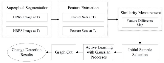
In change detection, we have discrete outputs (labels) $y\in \{\pm 1\}$ for “change” or “no change”. However, the actual outputs ${\mu }_{*}$ of active learning with Gaussian processes are continuous quantities between [−1, 1]. Without any constraint, the final change detection label of active learning is given by:

$$y=\left\{\begin{array}{cc}sign({\mu }_{*})\hfill & {\mu }_{*}\ne 0\hfill \\ -1\hfill & {\mu }_{*}=0\hfill \end{array}\right.$$

(4)

There is no spatial constraint between neighboring samples in this active learning process which only uses attribute information. To integrate the contextual information and attribute information, we formulate the change detection problem in a Bayesian framework [46], wherein the detection process is usually conducted by maximizing the posterior distribution as follows:

$$p(y|\mathbf{x})\propto p(\mathbf{x}|y)p(y)$$

(5)

where $p(\mathbf{x}|y)$ is the likehood measure (i.e., the probability of the pairwise feature images given the change results) and $p(y)$ is the prior change probability of pairwise images. Assuming conditional independence of the features given the change results [47], i.e., $p(\mathbf{x}|y)={\prod }_{i=1}^{i=n}p({\mathbf{x}}_{\mathbf{i}}|y_i),n$ is the number of samples, then the posterior results can be written as [34]:

$$\begin{array}{cc}\hfill p(y|\mathbf{x})& =\frac{1}{p(\mathbf{x})}p(x|y)p(y)\hfill \\ & =\frac{1}{p(\mathbf{x})}\prod _{i=1}^{i=n}p({\mathbf{x}}_{\mathbf{i}}|y_i)p(y)\hfill \\ & =\frac{{\prod }_{i=1}^{i=n}p({\mathbf{x}}_{\mathbf{i}})}{p(\mathbf{x})}\prod _{i=1}^{i=n}\frac{p(y_i|{\mathbf{x}}_{\mathbf{i}})}{p(y_i)}p(y)\hfill \end{array}$$

(6)

where $\frac{{\prod }_{i=1}^{i=n}p({\mathbf{x}}_{\mathbf{i}})}{p(\mathbf{x})}$ only depends on $\mathbf{x}$. Therefore, the MAP change detection can be formulated as:

$$\widehat{y}=argmax\{\sum _{i=1}^{n}logp(y_i|{\mathbf{x}}_{\mathbf{i}})+logp(y)\}$$

(7)

In this Bayesian framework, the attribute information is represented by $p(y_i|{\mathbf{x}}_{\mathbf{i}})$, which are computed by active learning with Gaussian processes. On the other hand, the spatial prior $p(y)$ is given by an MRF-based prior which assigns neighboring pixels with the same detection label. The MAP change detection $\widehat{y}$ can be computed by the $\alpha$-Expansion min-cut-based integer optimization algorithm [48].

3. Methodology

Object-based image analysis is a developing and promising alternative to pixel-based image analysis in that it integrates a broad spectrum of object features, therefore it is adopted for our purpose [49]. The whole framework flowchart is shown in Figure 1. The image over-segmentation and superpixel-based feature extraction are the essential steps for object-based analysis of HRRS imagery. Histogram intersection kernel [50] is used to obtain the feature difference map. In the presented method, there is no actual land cover category at the beginning. Thus we first use unsupervised k-means clustering to choose the nearest samples from the clustering centers, and to find a certain number of the most representative objects. Then these selected samples are labelled with “change” or “no change” by users as the initial training set. Next, we can detect the change areas from multi-temporal HRRS images by the active learning with Gaussian processes. The active learning framework stops when the detection result does not change notably or the number of iterations reaches a maximum. After we obtain the detection results of active learning, the contextual constraints are added via the MRF model. The final MAP output is computed by using graph cut.

3.1. Superpixel Segmentation

Existing superpixel segmentation algorithms can be divided into two categories: graph theory based algorithms and gradient descent based algorithms. By comparing the segmentation speed and segmentation results, we finally chose the Simple Linear Iteration Clustering (SLIC) segmentation algorithm [35]. This method can produce consistent superpixels with similar size and shape, and maintain image boundaries at the same time. Furthermore, the segmentation results are convenient for subsequent processing based on the well maintained boundaries.

In this step, the first remote sensing image in the multi-temporal series with complex boundaries is segmented into thousands of superpixels with SLIC. Then the superpixel segmentation result is applied to other temporal remote sensing images to keep the correspondence of superpixels in different images. The region size of superpixels can be set manually in experiments according to the resolution of images.

3.2. Feature Extraction

To distinguish whether the corresponding superpixels have changed, we first need to effectively describe all superpixels with their features. Because of the irregularity of over-segmented superpixels, the enclosing rectangle of each superpixel is taken into consideration. We calculate color and structure features of each rectangular region, then concatenate various features of the same region as the descriptor of that superpixel. Finally all descriptors of the same temporal remote sensing image constitute the feature set of that temporal image. To achieve the efficiency and discrimination of feature description, the discriminate color descriptor (DCD) [51] and scale-invariant feature transform (SIFT) [20] are utilized to represent color and structure information for each superpixel.

DCD represents color feature based on an information theory. RGB color values are clustered together based on their discriminative power in a classification problem [52], so that each cluster has the explicit objective to minimize the decline of mutual information of the final representation. Besides, this kind of color description can automatically maintain photometric invariance to some extent. Thus, we use a universal color representation, which is learned from natural image dataset in Google, to describe our superpixels. The specific theory and calculation process of DCD can be found in [51].

At the same time, we use SIFT descriptor of each superpixel to represent its texture information. The SIFT descriptor is in the modified version consisting of 32-dimension vectors [20]. Considering the superpixel segmentation result of the first temporal image is directly applied to the other images, the texture of superpixels in the first image is relatively homogeneous owing to the homogeneous superpixel segmentation algorithm, but the texture in the second images can be heterogeneous because some changes may occur in the homogeneous area. In other words, the SIFT descriptor is also useful in this scenario.

After calculating color and texture descriptors for all superpixels, all feature descriptors should be normalized according to their categories. The last procedure is concatenating the normalized color and SIFT descriptors to constitute descriptor sets for all temporal remote sensing images.

3.3. Similarity Measurement

To measure the similarity of superpixel pairs at the same location in different temporal remote sensing images, the histogram intersection kernel [53] of feature descriptor is calculated as the similarity metric. The histogram intersection kernel is defined as:

$${\mathbf{K}}^{hik}(\mathbf{x},{\mathbf{x}}^{\prime })=min(x_d,x_d^{\prime }),$$

(8)

where $\mathbf{x}$ and ${\mathbf{x}}^{\prime }$ are features of corresponding superpixels in different temporal remote sensing images, $x_d$ and $x_d^{\prime }$ are the d-th dimension of $\mathbf{x}$ and ${\mathbf{x}}^{\prime }$, ${\mathbf{K}}^{hik}$ is the histogram intersection kernel of feature vectors extracted in superpixel pairs. Thus, the similarity metric for each pair of superpixels in different temporal remote sensing images has the same dimension with descriptors for the original superpixels.

3.4. Initial Sample Selection

Before the active learning process, some samples should be selected to build the initial model, which means selecting the most representative samples from the original remote sensing image superpixel pairs using certain selection strategy. Without any category information, we try to use unsupervised means to choose “the most informative” samples and label them as the initial training set. In this study, k-means clustering is utilized to complete this task. Since the detection result is either “change” or “no change”, we choose the superpixel pairs nearest to the clustering centers found by k-means clustering algorithm ($k=2$) as the initial samples. All selected initial samples will be annotated by experts, which is simulated by actual change type in the following experiments.

3.5. Interactive Change Detection Based on Active Learning

Based on the initial two categories of samples, the change detection problem is treated as a two-category classification task. We use the labelled samples to train the Gaussian process model. Then according to Equations (1) and (2), we can calculate the predictive mean and variance of unlabelled samples. Next, active learning can train a more accurate Gaussian process model and improve the precision of change detection. Since HRRS images contain huge volumes of data, the process is very complex. To solve this problem, we use the rapid uncertainty computation with Gaussian processes [45] to implement the interactive change detection. The specific components of active learning with Gaussian processes are shown in Figure 2. We note that one of the significant advantages of Gaussian process is that it enables the estimation of classification uncertainties in a Bayesian manner.

The result for the classification problem of two categories in Gaussian processes is very simple, because the symbol of predictive mean directly reflects the classified category. However, the computation complexity of Gaussian processes is $O(n)$, which means it is not suitable for large scale classification problems. The utilization of Gaussian processes in large scale classification tasks becomes possible since Alexander et al. [45] proposed a series of optimization methods to reduce the computational complexity. The general idea is performing exact large-scale Gaussian process classification with parameterized histogram intersection kernels. The utilization of a full Bayesian model without any sparse approximation enables the learning in constant time. The specific optimization for rapid computation of Gaussian processes has been presented in [41], and the sample selection strategies based on rapid uncertainty computation with Gaussian processes is specified in the following part.

According to our previous work [54], we found that “the predictive mean”, “the uncertainty” and “impact on overall model change” are three relatively better and more stable query strategies for the change detection of HRRS images. Thus, we will review these sample selection strategies briefly and utilize them in experiments.

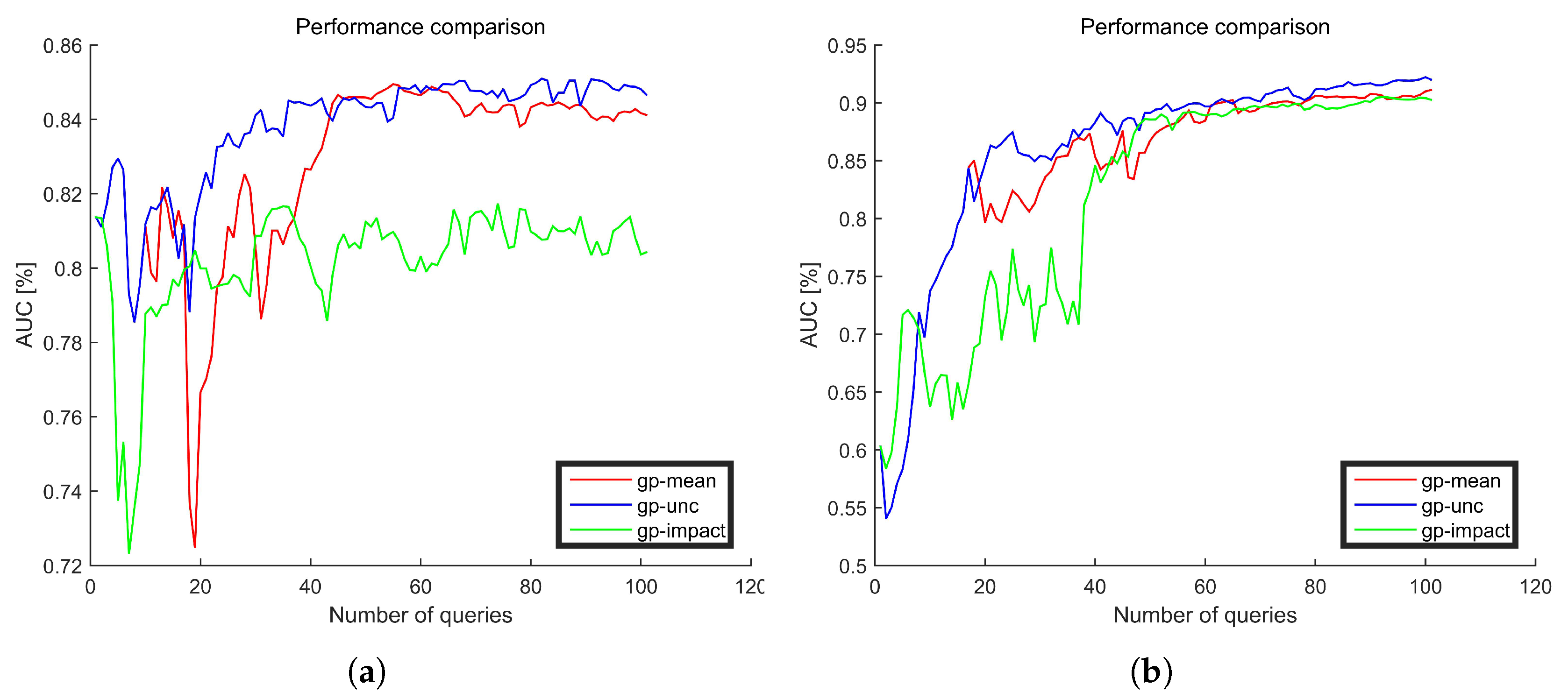
3.5.1. Sample Selection Criteria

• The predictive mean
  The predictive mean tries to select samples close to the current decision boundary, which belongs to exploitative methods. The predictive mean is given by

  $${\mathcal{Q}}_{{\mu }_{*}}(U)=arg\underset{{\mathbf{x}}_{\mathbf{i}}\in U}{min}\left|{\mu }_{*}({\mathbf{x}}_{\mathbf{i}})\right|,$$

  (9)

  where U is the feature set of unlabelled testing samples.
• The uncertainty
  The uncertainty tries to use the predictive mean and variance to select the most representative samples by making trade-offs between exploitative and explorative methods, which is given by

  $${\mathcal{Q}}_{unc}(U)=arg\underset{{\mathbf{x}}_{\mathbf{i}}\in U}{min}\frac{|{\mu }_{*}({\mathbf{x}}_{\mathbf{i}})|}{\sqrt{{\sigma }_{*}^2({\mathbf{x}}_{\mathbf{i}})}}.$$

  (10)
• Impact on the overall model change
  The impact [42] tries to choose the samples that will affect the current model heavily even with the most plausible label, which is given by

  $${\mathcal{Q}}_{impact}(U)=arg\underset{{\mathbf{x}}_{\mathbf{i}}\in U}{max}\underset{y^{(i)}\in \{\pm 1\}}{min}{∥\frac{|{\mu }_{*}({\mathbf{x}}_{\mathbf{i}})-y^{(i)}|}{{\sigma }_{*}^2({\mathbf{x}}^{*})}·\left[\begin{array}{c}{(\mathbf{K}+{\sigma }^2\mathbf{I})}^{-1}{k}_{*}\\ -1\end{array}\right]∥}_1.$$

  (11)

3.5.2. Labelling the Easiest Sample

In active learning process, “the most informative” sample in theory is chosen from an unlabelled dataset according to query strategies in each iteration. However, this sample is likely to be the most difficult one to distinguish by artificial selection even for professional experts. Thus, we can select some informative candidate samples, and then choose “the easiest” one to label without any uncertainty [55].

First, the new sample selection process chooses n candidate samples ${\mathbf{X}}_{\mathbf{n}}=\{{\mathbf{x}}_{\mathbf{1}},{\mathbf{x}}_{\mathbf{2}},\dots ,{\mathbf{x}}_{\mathbf{n}}\}$ according to different selecting strategies. Then, the “easiest” sample is selected based on the neighboring similarity. Comparing the similarity between candidate samples and their neighborhoods, we believe that a simple sample has high similarity to its surrounding superpixels. The similarity is defined as:

$$N(\mathbf{S},{\mathbf{x}}_{\mathbf{i}})=\sum _{j=1}^R{w}_{j}Sim({\mathbf{s}}_{\mathbf{j}},{\mathbf{x}}_{\mathbf{i}}),$$

(12)

where $\mathbf{S}=\{{\mathbf{s}}_{\mathbf{1}},{\mathbf{s}}_{\mathbf{2}},\dots ,{\mathbf{s}}_{\mathbf{R}}\}$ is the R neighborhoods of superpixel ${\mathbf{x}}_i$. $w_j=R-j+1$, which means the most similar neighborhood has the highest weight. $Sim({\mathbf{s}}_{\mathbf{j}},{\mathbf{x}}_{\mathbf{i}})$ is the Euclidean distance between every neighborhood and the candidate samples ${\mathbf{x}}_{\mathbf{i}}$. The smallest one is “the easiest” sample. We label it as “change” or “no change” sample, remove it from unlabelled samples and add to labelled dataset iteratively.

3.6. Refinement with MRF Via Graph Cuts

After interactive change detection using active learning, the outputs $u_{*}$ are distributed in $[-1,+1]$. The closer the value is to $+1$, the more likely the corresponding superpixel has changed. Thus, the individual change probability can be formulated as:

$$p(y_i|{\mathbf{x}}_{\mathbf{i}})=\frac{u_{*}^i+1}{2}$$

(13)

where $u_{*}^i$ is the predicted mean value of Gaussian processes of $i_{th}$ superpixel. Until now, we have obtained the change probability map of all superpixels in the HRRS images, which has fully used the attribute information. To simplify the neighbor relationship of individual pixels, the change probabilities of superpixels are mapped to every pixel in the original image and the MRF model is formulated at pixel-level. Thus the spatial information can be easily applied by the four neighboring domains.

According to the MRF-based spatial prior [34], the spatial constraints with an MRF can be modeled as,

$$p(y)=\frac{1}{Z}{e}^{\mu {\sum }_{(i,j)\in \zeta }\delta (y_i-y_j)}$$

(14)

where Z is a normalizing constant, $(i,j)\in \zeta$ forms the spatial adjacent constraints, and $\delta (y)$ is the unit impulse function. The constraint in Equation (14) indicates that neighbors should have the same change result. The pairwise interaction terms $\delta (y_i-y_j)$ attach higher probability to equal neighboring labels than the reverse. In this way, the multilevel logistic (MLL) prior on image labels promotes piecewise smooth change detection, where $\mu$ is a nonnegative constant which controls the level of smoothness.

To integrate the attribute information $p(y_i|{\mathbf{x}}_{\mathbf{i}})$ and contextual information $p(y)$, the MAP change detection Equation (7) can be rewritten as:

$$\widehat{y}=argmin\{\sum _{i\in S}-logp(y_i|{\mathbf{x}}_{\mathbf{i}})-\mu \sum _{(i,j)\in \zeta }\delta (y_i-y_j)\}$$

(15)

This formulation is a typical MRF problem: ${\sum }_{i\in S}-logp(y_i|{\mathbf{x}}_{\mathbf{i}})$ is the data term, and ${\sum }_{(i,j)\in \zeta }\delta (y_i-y_j)$ is the smooth term. In this paper, we utilize the $\alpha$-Expansion graph-cut-based algorithm [48], which yields good approximations to the MAP change detection. More importantly, this method is quite efficient with the computational complexity $O(n)$, since it can well handle the data complexity increase caused by the analysis from superpixel level to pixel level. The final outputs are the change labels of all pixels in the HRRS image.

4. Experiments

In this section, we test the proposed interactive change detection method on several HRRS images. The experimental results demonstrate the benefits of our active learning method with MRFs for change detection. In these experiments, we can choose any of the query strategies listed above. All those chosen representative samples will be added into the training set after labelling, which is compared with classical SVM classifiers and actual land cover change truth. After that, we briefly test the results of the integration of attribute information and contextual information. Additionally, we compare the original sample selection strategies and the improved sample selection with labelling the easiest sample of active learning. In the experimental results, the most common used change detection indexes, i.e., the overall detection accuracy (OA), detection precision for change area (Pc), detection precision for no-change area (Pu) and Kappa coefficient (KC) are calculated to demonstrate the effectiveness of our methods. The main subsections are reported in the following three parts: (1) introduce the experimental data; (2) present the experimental settings; and (3) analyze the experimental results.

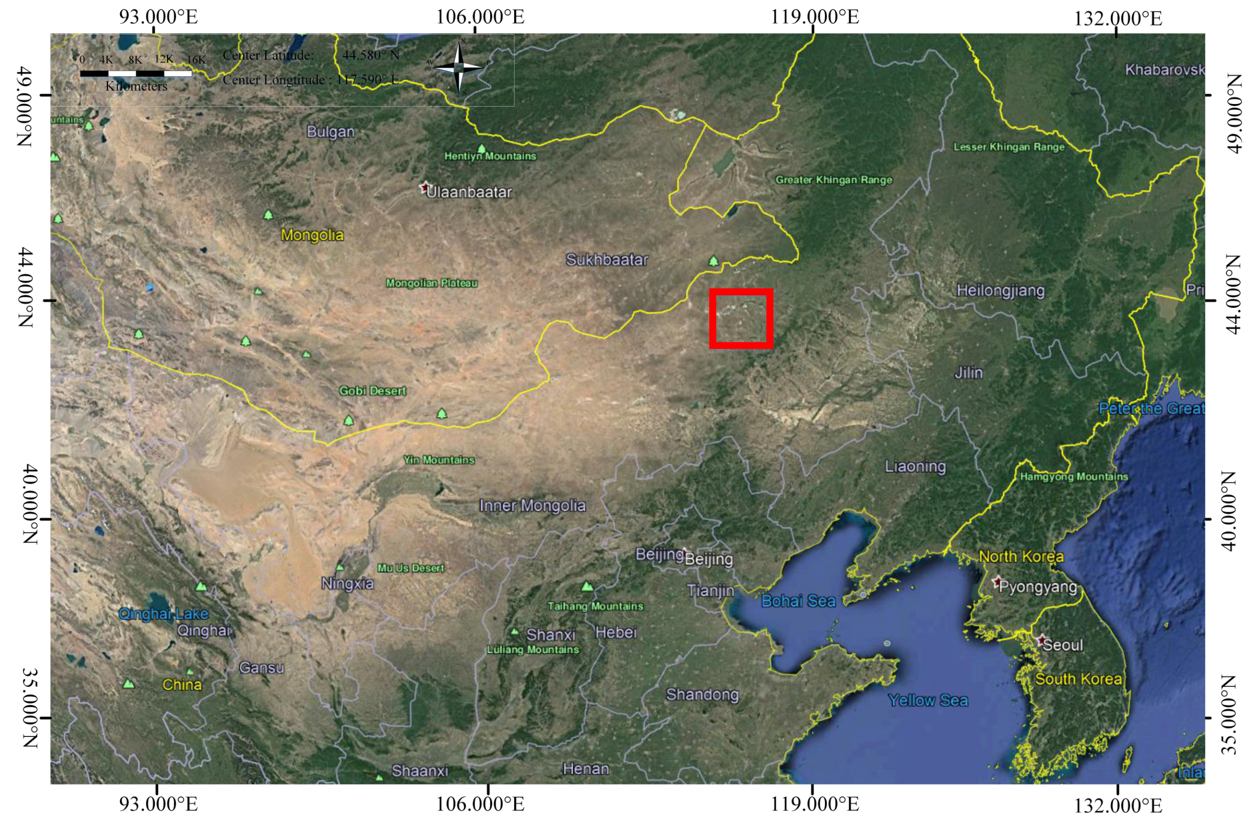
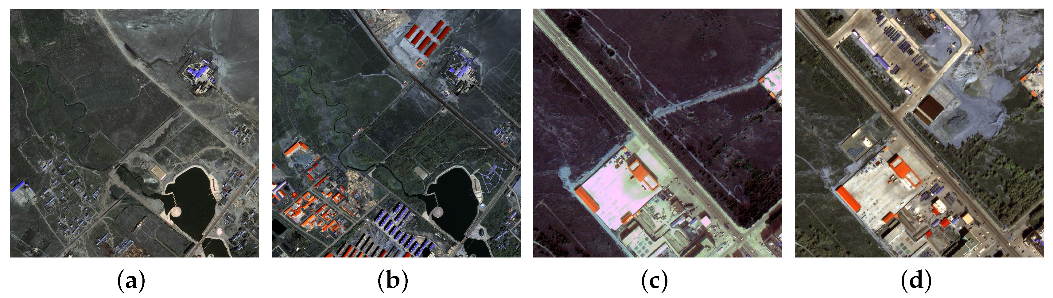
4.1. The Experimental Datasets

We test the proposed method on two sets of WorldView-2 HRRS images. WorldView-2 is a commercial Earth observation satellite, which provides panchromatic imagery of 0.46 m resolution and eight-band multispectral imagery with 1.84 m resolution. It was launched 8 October 2009 and could acquire a new image of any place on the Earth every 1.1 days. The resolution of panchromatic image is relatively higher than multispectral data, and we can obtain a new HRRS image with multi-spectral information by pansharping of green, blue and red bands and radiometric correction. There are two temporal images including green, blue and red bands in each image set. The research area is located in Xilinhaote-Xiwuqi, central Inner Mongolia of China (in Figure 3, red box). The first dataset covers grassland, buildings and lake with size of 3000 × 3000 pixels and resolution of 0.5 m. The main change type is the change from grassland to buildings. Figure 4a shows the image on 18 September, 2013 and Figure 4b shows the image on 12 September, 2015. The second dataset covers road, buildings and grassland and bareland with size of 1000 × 1000 pixels and resolution of 0.5 m. The main change type is the change from grassland to bareland. This dataset is shown in Figure 4c,d with the same time, respectively.

4.2. The Experimental Setup

To conduct our proposed methods, some essential steps and key parameters should be clear. The superpixel segmentation process is the basic process to obtain the regular and homogeneous objects. In our experiments, we use VLFeat open source library (http://www.vlfeat.org/overview/slic.html) to implement the process. The two parameters (regionSize and regularizer) are empirically set as 15 and 0.1, respectively. The regionSize is related to the resolution of images and the general meaningful region size. The regularizer is related to the texture resolution of images. To express the information of every object, we use the concatenation of color [51] and texture features [20], which results in a 82 dimensional vector. For the labelling process in active learning, we label the change truth of the corresponding superpixels when the sample selection process identifies the most informative samples. The GUI interface will simultaneously display the two corresponding selected samples for experts. The labelling process is to select $-1$ for “no change ” and 1 for “change”, which is very easy to implement. To demonstrate the effectiveness of the proposed active learning method for change detection, we compare our method to the typical supervised change detection method, i.e., SVM based classifiers with intersection kernel [50], and several typical unsupervised change detection methods, KI threshold [56], Otsu threshold [57], CVA [58] and IR-MAD [26] methods. In the interactive change detection of active learning, the number of iterations is set to 100, which means that we at most use 104 training samples (including the two changed and two unchanged samples in the initial sample selection process) to conduct the change detection. For active learning with Gaussian processes, we also present the performance of different sample selection strategies. For the MAP change detection with the contextual constraints, the smooth parameter is set $\mu =2$ as an empirical value.

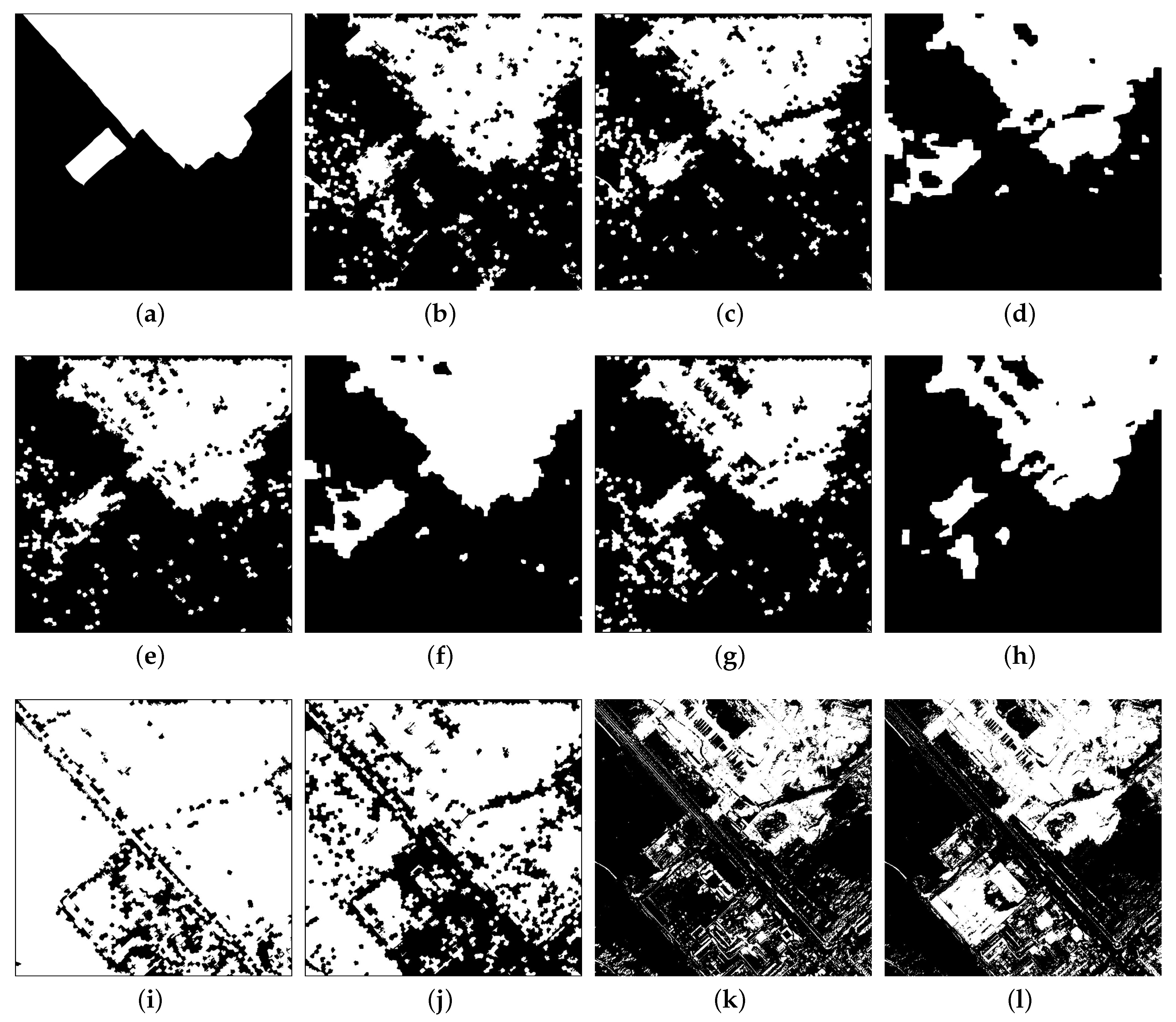
4.3. Experimental Results

In this section, we show the experimental results on the above mentioned two datasets and analyze the details about our active learning methods compared with some representative competitors. Figure 5 shows the detection results of change areas for Datset 1. Figure 5a is the change ground truth for Datset 1 in which white means change and black means no-change. Figure 5b is the detection result using SVM. It should be mentioned that by using the same number of training samples, for the supervised method with SVM classifier, we randomly select training samples 100 times and choose the best one (with the highest performance) to obtain the result shown in Figure 5b. Figure 5c,e,g shows the active learning based change detection results of different sample selection strategies, the predictive mean, the uncertainty and impact on the overall model change respectively. Figure 5d,f,h shows the MAP change detection results with the three sample selection strategies. Through the qualitative comparison of the performance of the three different sample selection strategies, the result of uncertainty (Figure 5e) shows the best performance. After adding the contextual constraints, the MAP detection results are relatively better than the pure active learning method regardless of sample selection strategies. Compared with typical supervised method, i.e., SVM classifier, the active learning frameworks are also more competitive. Compared with conventional unsupervised methods, Figure 5i–l shows the results of KI threshold, Otsu threshold, CVA and IR-MAD method. We can see that many change areas are wrongly detected as non-change areas of KI threshold. However the results of Otsu threshold are just the opposite, many non-change areas are wrongly detected as change areas, while the CVA and IR-MAD methods show better results considering the structure of changed areas. Comparing IR-MAD and active learning based on uncertainty (no spatial information), the results are very similar and further analysis is needed.

To further analyze the experimental results,

Table 1. The comparison of different change detection results for Datset 1.

Strategy	OA	Pc	Pu	Kappa
SVM	0.7459	0.6296	0.8116	0.4448
AL Mean	0.7593	0.6795	0.8043	0.4811
AL Mean MRF	0.7921	0.7405	0.8213	0.5550
AL Uncertainty	0.7764	0.7222	0.8070	0.5220
AL Uncertainty MRF	0.8040	0.7572	0.8304	0.5803
AL Impact	0.7527	0.6579	0.8062	0.4640
AL Impact MRF	0.7134	0.3209	0.9352	0.2920
KI Threshold	0.6285	0.6418	0.6209	0.2460
Otsu Threshold	0.6728	0.2036	0.9379	0.1663
CVA	0.7664	0.5136	0.9092	0.4550
IR-MAD	0.7613	0.7006	0.7956	0.4895

presents the quantitative performance indexes of these different methods for Datset 1. Without considering the contextual information, we first compare the active learning methods with other supervised and unsupervised methods. Actually, for the SVM classifier, we repeated the experiment 100 times, the average detection accuracy (OA) is $0.7099\pm 0.0231$. The results of SVM classifier in Table 1 (OA = 0.7459) is the best one among the 100 times, which is still inferior to the active learning method with the uncertainty (OA = 0.7764). In addition, for the random selection of training samples, the results of SVM classifiers fluctuate in a wide range. On the contrary, the results of active learning do not change for the same sample selection strategy. Among the three different sample selection strategies, the OA and KC of active learning based on uncertainty are the highest, which is consistent with the results of qualitative analysis. In addition, compared with the unsupervised methods, the detection precision indexes for change area (Pc) and no-change area (Pu) of change detection based on active learning are much higher than the KI and Otsu thresholds. Then compared with the best one, i.e., IR-MAD, among the four unsupervised methods, our active learning framework based on uncertainty (AL Uncertainty) is still better in terms of OA, Pc, Pu and KC indexes. Furthermore, after the integration of attribute information and contextual information, the MAP change detection results are much better compared with the pure active learning method except for the impact sample selection strategy. Analyzing the qualitative results in Figure 5g,h, we can find that many isolated changed superpixels are fused in the unchange area, so the Pc for the AL Impact MRF method (0.3209) is much smaller than that for the AL Impact method (0.6579). Therefore, with the help of limited reliable labelled samples, the active learning framework for change detection can be superior to typical unsupervised and supervised methods.

Figure 6 shows the results for Dataset 2. The sub-figures are the corresponding results as Figure 5.

Table 2. The comparison of different change detection results for Dataset 2.

Strategy	OA	Pc	Pu	Kappa
SVM	0.8717	0.8603	0.8771	0.7153
AL Mean	0.8623	0.7657	0.9176	0.6967
AL Mean MRF	0.9276	0.8909	0.9451	0.8347
AL Uncertainty	0.8748	0.7889	0.9240	0.7251
AL Uncertainty MRF	0.9442	0.9538	0.9396	0.8750
AL Impact	0.8505	0.7615	0.9015	0.6725
AL Impact MRF	0.9291	0.8409	0.9713	0.8337
KI Threshold	0.4736	0.9678	0.1907	0.1223
Otsu Threshold	0.6122	0.8570	0.4721	0.2821
CVA	0.8139	0.6676	0.8837	0.5644
IR-MAD	0.7997	0.7471	0.8249	0.5554

shows the quantitative analysis indexes of different change detection methods. By observing the results of the three different sample selection strategies in Figure 6, we can still find that the active learning based on the uncertainty is the most similar one to the change ground truth. For the SVM classifier, the average accuracy is $0.8370\pm 0.0315$. Comparing with SVM classifier and unsupervised methods, our active learning methods show better performance. Although the indexes of SVM in Table 2 are also competitive, it is the best realized result among 100 times. The random selection of samples leads to unstable results, while the performances of active learning are very stable. Table 2 also indicates that active learning based on the uncertainty has the highest OA and KC indexes, reaching 0.8748 and 0.7251 respectively. In addition, the results of change detection methods based on active learning are much better than the unsupervised ways. In IR-MAD method, a large flatland is misclassified as changed area (see Figure 6l).By observing the original two images, we can find that these misclassified changed areas actually are in different illumination. After adding the contextual constraints, the MAP change detection results are more convincing, the OA and Kappa coefficient of AL Uncertainty MRF achieves 0.9442 and 0.8750 respectively. Therefore, our change detection framework based on active learning and MRFs is more practical in actual circumstances.

By selecting the most informative samples to train the active learning model, our interactive framework performs very well in the detection of change areas of HRRS images. The results of the AL methods are very stable as compared to the unstable SVM classifier. Compared with typical supervised and unsupervised change detection methods, our active learning method uses very limited training samples, but it yields much better results. In addition, the integration of attribute information and contextual information further improves the change detection results.

5. Discussion

Change detection is a very important issue in the interpretation of multi-temporal HRRS imagery. In this paper, we firstly analyze the pros and cons of the typical supervised and unsupervised change detection methods and then we introduce an interactive change detection method based on active learning and MRFs. The objective is to use active learning to find the most informative samples and obtain the best change detection results. In our experiments, we use three different sample selection strategies to test the performance, and find out that the uncertainty measure can find the most informative samples under the same iteration setting. In our method, the manual annotation can be reduced substantially, and after the integration of attribute information and contextual information, a desirable detection result can be obtained.

In the original active learning model, based on the sample selection criteria in Section 3.5.1, the most informative sample is the one in the front of the queue. However, this sample is often very difficult to label even for experts, but the labelling is the key problem for a good detection result. Thus we first select the front m (e.g., $m=10$) samples from the queue, and then select the most distinguished one for manually annotation from these candidates. This strategy is called labelling the easiest sample, which is described in Section 3.5.2.

Table 3. The comparison of improved active learning with the original active learning.

	Strategy	OA	Pc	Pu	Kappa
Dataset 1	Original AL	0.7609	0.7280	0.7795	0.4947
	Improved AL	0.7764	0.7222	0.8070	0.5220
	Improved AL MRF	0.8040	0.7572	0.8304	0.5803
Dataset 2	Original AL	0.8658	0.7921	0.9079	0.7072
	Improved AL	0.8748	0.7889	0.9240	0.7251
	Improved AL MRF	0.9442	0.9538	0.9396	0.8750

shows the comparison of change detection results of the original active learning with our improved one. Under the same sample selection criterion, i.e., the uncertainty, the performance indexes of our improved active learning is relatively better than the original one on the two datasets, especially the Kappa coefficient, about 2.7% higher and 1.8%, respectively. Although this treatment does not change the essence of annotation, it makes the labelling more reliable. In addition, the spatial constraints using contextual information also greatly promote the performance, increasing the Kappa coefficient by 5.8% and 14.99%, respectively.

To further compare the change detection results, the McNemar test was employed [59]. The confusion matrix is formed based on the agreements and disagreements of AL Uncertainty MRF and the other one method. The difference between two methods is significant when the test index, p-value is less than 0.05. The proposed method (AL Uncertainty MRF) is compared with five representative methods, i.e., the typical supervised method (SVM), AL Uncertainty, AL Mean MRF, AL Impact MRF and the typical unsupervised method (IR-MAD).

Table 4. The McNemar’s test between AL Uncertainty MRF with other five methods for Datset 1.

Method	${\mathit{f}}_{\mathbf{11}}\mathbf{\times }{\mathbf{10}}^{\mathbf{6}}$	${\mathit{f}}_{\mathbf{12}}\mathbf{\times }{\mathbf{10}}^{\mathbf{6}}$	${\mathit{f}}_{\mathbf{21}}\mathbf{\times }{\mathbf{10}}^{\mathbf{6}}$	${\mathit{f}}_{\mathbf{22}}\mathbf{\times }{\mathbf{10}}^{\mathbf{6}}$	${\mathit{\chi }}^{\mathbf{2}}\mathbf{\times }{\mathbf{10}}^{\mathbf{6}}$	p
SVM	1.1465	1.1408	0.6182	6.0944	0.1553	<0.001
AL Uncertainty	1.2969	0.7583	0.4678	6.4769	0.0688	<0.001
AL Mean MRF	1.3771	0.4938	0.3877	6.7414	0.0128	<0.001
AL Impact MRF	1.0087	1.5700	0.7560	5.6652	0.2848	<0.001
IR-MAD	0.8803	1.2680	0.8844	5.9673	0.0683	<0.001

and

Table 5. The McNemar’s test between AL Uncertainty MRF with other five methods for Dataset 2.

Method	${\mathit{f}}_{\mathbf{11}}\mathbf{\times }{\mathbf{10}}^{\mathbf{5}}$	${\mathit{f}}_{\mathbf{12}}\mathbf{\times }{\mathbf{10}}^{\mathbf{5}}$	${\mathit{f}}_{\mathbf{21}}\mathbf{\times }{\mathbf{10}}^{\mathbf{5}}$	${\mathit{f}}_{\mathbf{22}}\mathbf{\times }{\mathbf{10}}^{\mathbf{5}}$	${\mathit{\chi }}^{\mathbf{2}}\mathbf{\times }{\mathbf{10}}^{\mathbf{5}}$	p
SVM	0.2702	1.0165	0.2872	8.4261	0.4079	<0.001
AL Uncertainty	0.3306	0.8939	0.2269	8.5486	0.3970	<0.001
AL Mean MRF	0.3553	0.3626	0.2022	9.0799	0.0456	<0.001
AL Impact MRF	0.2181	0.4818	0.3393	8.9607	0.0247	<0.001
IR-MAD	0.1798	1.8189	0.3777	7.6237	0.9456	<0.001

are the McNemar’s test results for Datset 1 and Dataset 2, respectively. $f_{11}$ denotes the number of pixels with the wrong detection for both AL Uncertainty MRF and other methods, $f_{12}$ denotes the number of pixels that are correctly detected by AL Uncertainty MRF but wrongly detected by the other, $f_{21}$ denotes the number of pixels that are wrongly detected by AL Uncertainty MRF but correctly detected by the other, and $f_{22}$ is the number of pixels with the correct detection in both methods. Compared with the typical supervised and unsupervised methods (SVM and IR-MAD), the proposed AL Uncertainty MRF is much better. Compared with the improved AL Uncertainty, AL Uncertainty MRF also shows better performance, which illustrates the effectiveness of combining MRF. Furthermore, by comparing the active learning methods based on different sample selection strategies, we can also observe that the method based on uncertainty is the best one. In summary, the McNemar’s tests further show significant improvement of the AL Uncertainty MRF based method over the other five methods.

The above described active learning methods are all conducted on proper settings of parameters (Section 4.2). The two key parameters for our method are object size and the number of iterations. The size of objects are obtained empirically, which is also related to the image resolution. Pixel-based change detection can also work with this active learning framework, but it is very time consuming. Figure 7 shows the gains of active learning after different number of iterations. Accuracies after every query are evaluated on disjoint test set using the area under receiver operator curves (AUC). Generally, the accuracy index first increases and then keeps stable with the increase of the number of iterations. There are some performance fluctuations for small numbers of iterations. The reason is that every added training sample plays a very important role in the model training when the number of samples is small. Thus if an inaccurate sample is selected for training the model, the performance will degrade. However, when the number of iterations is larger, the effect of limited inaccurate samples can also be reduced. This is why the performance finally improved. Generally, the performances of the Gaussian process based on the uncertainty (gp-unc, in blue) are relatively better than the Gaussian process based on the mean value (gp-mean, in red) for both two datasets. When adding a new training sample, the performance gains of different query strategies vary. Thus, adding new samples when the training sample set is not complete, the performance gain of gp-mean maybe better than gp-unc. However, after we add enough and complete training samples, the performances of different query strategies trend to be stable and the performance of gp-unc is relatively better than gp-mean (after number of queries above 80).

6. Conclusions

In this paper, an interactive change detection method has been proposed to detect changes of multi-temporal HRRS images using active learning and MRFs. The main contributions are twofold. We first use active learning with Gaussian processes to iteratively optimize the detection model, which address three different sample selection strategies with labelling the easiest sample. Then, we integrate attribute (color and texture) information and contextual information into the MRFs, so that the MAP change detection can be efficiently computed via the min-cut-based integer optimization algorithm. With the active learning framework and MRFs, our method can achieve competitive detection results using very limited training samples. Both qualitative and quantitative analyses of the experimental results demonstrate the satisfactory performance of the proposed change detection framework. In the experiment, we also observe that the uncertainty is the relatively better and more stable query strategy for the change detection of HRRS images. By using the contextual constraints, the posterior detection results can be more competitive with the state-of-the-art. In the future, we intend to explore more stable and discriminative sample selection strategies and extend our methods to SAR image change detection.

References

1. Singh, A. Digital change detection techniques using remotely sensed data. Int. J. Remote Sens. 1988, 10, 989–1003. [Google Scholar] [CrossRef]
2. Büttner, G. Corine land cover and land cover change products. In Land Use and Land Cover Mapping in Europe; Springer: Houten, The Netherlands, 2014; pp. 55–74. [Google Scholar]
3. Ma, Y.; Chen, F.; Liu, J.; He, Y.; Duan, J.; Li, X. An automatic procedure for early disaster change mapping based on optical remote sensing. Remote Sens. 2016, 8, 272. [Google Scholar] [CrossRef]
4. Schroeder, T.A.; Healey, S.P.; Moisen, G.G.; Frescino, T.S.; Cohen, W.B.; Huang, C.; Kennedy, R.E.; Yang, Z. Improving estimates of forest disturbance by combining observations from Landsat time series with US Forest Service Forest Inventory and Analysis data. Remote Sens. Environ. 2014, 154, 61–73. [Google Scholar] [CrossRef]
5. Dewi, R.S.; Bijker, W.; Stein, A.; Marfai, M.A. Fuzzy classification for shoreline change monitoring in a part of the northern coastal area of Java, Indonesia. Remote Sens. 2016, 8, 190. [Google Scholar] [CrossRef]
6. Liu, D.; Cai, S. A spatial-temporal modeling approach to reconstructing land-cover change trajectories from multi-temporal satellite imagery. Ann. Assoc. Am. Geogr. 2012, 102, 1329–1347. [Google Scholar] [CrossRef]
7. Kennedy, R.E.; Yang, Z.; Cohen, W.B. Detecting trends in forest disturbance and recovery using yearly Landsat time series: 1. LandTrendr—Temporal segmentation algorithms. Remote Sens. Environ. 2010, 114, 2897–2910. [Google Scholar] [CrossRef]
8. Klonus, S.; Tomowski, D.; Ehlers, M.; Reinartz, P.; Michel, U. Combined edge segment texture analysis for the detection of damaged buildings in crisis areas. IEEE J. Sel. Top. Appl. Earth Obs. Remote Sens. 2012, 5, 1118–1128. [Google Scholar] [CrossRef] [Green Version]
9. Simard, M.; Saatchi, S.S.; De Grandi, G. The use of decision tree and multiscale texture for classification of JERS-1 SAR data over tropical forest. IEEE Trans. Geosci. Remote Sens. 2000, 38, 2310–2321. [Google Scholar] [CrossRef]
10. Hussain, M.; Chen, D.; Cheng, A.; Wei, H.; Stanley, D. Change detection from remotely sensed images: From pixel-based to object-based approaches. ISPRS J. Photogramm. Remote Sens. 2013, 80, 91–106. [Google Scholar] [CrossRef]
11. Leichtle, T.; Geiß, C.; Wurm, M.; Lakes, T.; Taubenböck, H. Unsupervised change detection in VHR remote sensing imagery – An object-based clustering approach in a dynamic urban environment. Int. J. Appl. Earth Obs. Geoinf. 2017, 54, 15–27. [Google Scholar] [CrossRef]
12. Yousif, O.; Ban, Y. Improving SAR-based urban change detection by combining MAP-MRF classifier and nonlocal means similarity weights. IEEE J. Sel. Top. Appl. Earth Obs. Remote Sens. 2014, 7, 4288–4300. [Google Scholar] [CrossRef]
13. Castellana, L.; D’Addabbo, A.; Pasquariello, G. A composed supervised/unsupervised approach to improve change detection from remote sensing. Pattern Recognit. Lett. 2007, 28, 405–413. [Google Scholar] [CrossRef]
14. Bovolo, F.; Bruzzone, L. The time variable in data fusion: A change detection perspective. IEEE Geosci. Remote Sens. Mag. 2015, 3, 8–26. [Google Scholar] [CrossRef]
15. Camps-Valls, G.; Gómez-Chova, L.; Munoz-Marí, J.; Rojo-Álvarez, J.L.; Martínez-Ramón, M. Kernel-based framework for multitemporal and multisource remote sensing data classification and change detection. IEEE Trans. Geosci. Remote Sens. 2008, 46, 1822–1835. [Google Scholar] [CrossRef] [Green Version]
16. Pons, X. Post-classification change detection with data from different sensors: Some accuracy considerations. Int. J. Remote Sens. 2003, 24, 4975–4976. [Google Scholar]
17. Ling, F.; Li, W.; Du, Y.; Li, X. Land cover change mapping at the subpixel scale with different spatial-resolution remotely sensed imagery. IEEE Geosci. Remote Sens. Lett. 2010, 8, 182–186. [Google Scholar] [CrossRef]
18. Molina, I.; Martinez, E.; Morillo, C.; Velasco, J.; Jara, A. Assessment of data fusion algorithms for earth observation change detection processes. Sensors 2016, 16, 1621. [Google Scholar] [CrossRef] [PubMed]
19. Wu, C.; Zhang, L.; Zhang, L. A scene change detection framework for multi-temporal very high resolution remote sensing images. Sign. Process. 2016, 124, 184–197. [Google Scholar] [CrossRef]
20. Lazebnik, S.; Schmid, C.; Ponce, J. Beyond bags of features: Spatial pyramid matching for recognizing natural scene categories. In Proceedings of the IEEE Computer Society Conference on Computer Vision & Pattern Recognition, New York, NY, USA, 17–22 June 2006; pp. 2169–2178. [Google Scholar]
21. Bruzzone, L.; Serpico, S.B. An iterative technique for the detection of land-cover transitions in multitemporal remote-sensing images. IEEE Trans. Geosci. Remote Sens. 1997, 35, 858–867. [Google Scholar] [CrossRef]
22. Volpi, M.; Tuia, D.; Bovolo, F.; Kanevski, M.; Bruzzone, L. Supervised change detection in VHR images using contextual information and support vector machines. Int. J. Appl. Earth Obs. Geoinf. 2013, 20, 77–85. [Google Scholar] [CrossRef]
23. Shao, P.; Shi, W.; He, P.; Hao, M.; Zhang, X. Novel approach to unsupervised change detection based on a robust semi-supervised FCM clustering algorithm. Remote Sens. 2016, 8, 264. [Google Scholar] [CrossRef]
24. Chen, K.; Zhou, Z.; Huo, C.; Sun, X.; Fu, K. A semisupervised context-sensitive change detection technique via gaussian process. IEEE Geosci. Remote Sens. Lett. 2013, 10, 236–240. [Google Scholar] [CrossRef]
25. An, L.; Li, M.; Zhang, P.; Wu, Y.; Jia, L.; Song, W. Discriminative random fields based on maximum entropy principle for semisupervised SAR image change detection. IEEE J. Sel. Top. Appl. Earth Obs. Remote Sens. 2016, 9, 3395–3404. [Google Scholar] [CrossRef]
26. Nielsen, A.A. The regularized iteratively reweighted MAD method for change detection in multi- and hyperspectral data. IEEE Trans. Image Process. 2007, 16, 463–478. [Google Scholar] [CrossRef] [PubMed]
27. Marpu, P.R.; Gamba, P.; Canty, M.J. Improving change detection results of IR-MAD by eliminating strong changes. IEEE Geosci. Remote Sens. Lett. 2011, 8, 799–803. [Google Scholar] [CrossRef]
28. Liu, S.; Bruzzone, L.; Bovolo, F.; Du, P. Hierarchical unsupervised change detection in multitemporal hyperspectral images. IEEE Trans. Geosci. Remote Sens. 2015, 53, 244–260. [Google Scholar]
29. Byun, Y.; Han, Y.; Chae, T. Image fusion-based change detection for flood extent extraction using bi-temporal very high-resolution satellite images. Remote Sens. 2015, 7, 10347–10363. [Google Scholar] [CrossRef]
30. Shah-Hosseini, R.; Homayouni, S.; Safari, A. A hybrid kernel-based change detection method for remotely sensed data in a similarity space. Remote Sens. 2015, 7, 12829–12858. [Google Scholar] [CrossRef]
31. Sinha, P.; Kumar, L.; Reid, N. Rank-based methods for selection of landscape metrics for land cover pattern change detection. Remote Sens. 2016, 8, 107. [Google Scholar] [CrossRef]
32. Zhu, G.; Wang, Q.; Yuan, Y.; Yan, P. Learning saliency by MRF and differential threshold. IEEE Trans. Cybern. 2013, 43, 2032–2043. [Google Scholar] [CrossRef] [PubMed]
33. Yuan, Y.; Lin, J.; Wang, Q. Hyperspectral image classification via multitask joint sparse representation and stepwise MRF optimization. IEEE Trans. Cybern. 2016, 46, 2966–2977. [Google Scholar] [CrossRef] [PubMed]
34. Li, J.; Bioucas-Dias, J.M.; Plaza, A. Spectral-spatial hyperspectral image segmentation using subspace multinomial logistic regression and markov random fields. IEEE Trans. Geosc. Remote Sens. 2012, 50, 809–823. [Google Scholar] [CrossRef]
35. Achanta, R.; Shaji, A.; Smith, K.; Lucchi, A.; Fua, P.; Süsstrunk, S. SLIC superpixels compared to state-of-the-art superpixel methods. IEEE Trans. Pattern Anal. Mach. Intell. 2012, 34, 2274–2282. [Google Scholar] [CrossRef] [PubMed]
36. Seo, S.; Wallat, M.; Graepel, T.; Obermayer, K. Gaussian Process Regression: Active Data Selection and Test Point Rejection; Springer: Berlin/Heidelberg, Germany, 2000; Volume 3, pp. 241–246. [Google Scholar]
37. MacKay, D.J.C. Information-based objective functions for active data selection. Neural Comput. 1992, 4, 590–604. [Google Scholar] [CrossRef]
38. Cohn, D.; Atlas, L.; Ladner, R. Improving generalization with active learning. Mach. Learn. 1994, 15, 201–221. [Google Scholar] [CrossRef]
39. Tuia, D.; Volpi, M.; Copa, L.; Kanevski, M.; Munoz-Mari, J. A survey of active learning algorithms for supervised remote sensing image classification. IEEE J. Sel. Top. Sign. Process. 2011, 5, 606–617. [Google Scholar] [CrossRef]
40. Sun, L.L.; Wang, X.Z. A survey on active learning strategy. In Proceedings of the International Conference on Machine Learning & Cybernetics, Qingdao, China, 11–14 July 2010; pp. 161–166. [Google Scholar]
41. Rodner, E.; Freytag, A.; Bodesheim, P.; Denzler, J. Large-scale gaussian process classification with flexible adaptive histogram kernels. In Proceedings of the European Conference on Computer Vision, Florence, Italy, 7–13 October 2012; pp. 85–98. [Google Scholar]
42. Freytag, A.; Rodner, E.; Bodesheim, P.; Denzler, J. Labeling examples that matter: Relevance-based active learning with gaussian processes. In Proceedings of the German Conference on Pattern Recognition, Saarbrücken, German, 3–6 September 2013; pp. 282–291. [Google Scholar]
43. Christoph, K.; Alexander, F.; Erik, R.; Paul, B.; Joachim, D. Active learning and discovery of object categories in the presence of unnamable instances. In Proceedings of the IEEE Conference on Computer Vision and Pattern Recognition, Boston, MA, USA, 7–12 June 2015; pp. 4343–4352. [Google Scholar]
44. Rodner, E.; Freytag, A.; Bodesheim, P.; Fröhlich, B.; Denzler, J. Large-scale gaussian process inference with generalized histogram intersection kernels for visual recognition tasks. Int. J. Comput. Vis. 2017, 121, 235–280. [Google Scholar] [CrossRef]
45. Freytag, A.; Rodner, E.; Bodesheim, P.; Denzler, J. Rapid uncertainty computation with gaussian processes and histogram intersection kernels. In Proceedings of the Asian Conference on Computer Vision, Daejeon, Korea, 5–9 November 2012; pp. 511–524. [Google Scholar]
46. Yang, W.; Dai, D.; Triggs, B.; Xia, G.S. SAR-based terrain classification using weakly supervised hierarchical Markov aspect models. IEEE Trans. Image Process. 2012, 21, 4232–4243. [Google Scholar] [CrossRef] [PubMed]
47. Jarecki, J.B.; Meder, B.; Nelson, J.D. Naïve and robust: Class-conditional independence in human classification learning. Cogn. Sci. 2017, 3, 1–39. [Google Scholar] [CrossRef] [PubMed]
48. Boykov, Y.; Veksler, O.; Zabih, R. Fast approximate energy minimization via graph cuts. IEEE Trans. Pattern Anal. Mach. Intell. 2001, 23, 1222–1239. [Google Scholar] [CrossRef]
49. Yu, H.; Yan, T.; Yang, W.; Zheng, H. An integrative object-based image analysis workflow for uav images. ISPRS Arch. Photogramm. Remote Sens. Spat. Inf. Sci. 2016, XLI-B1, 1085–1091. [Google Scholar] [CrossRef]
50. Barla, A.; Odone, F.; Verri, A. Histogram intersection kernel for image classification. In Proceedings of the IEEE International Conference on Image Processing, Barcelona, Spain, 14–17 September 2003; pp. 513–516. [Google Scholar]
51. Khan, R.; Van de Weijer, J.; Shahbaz Khan, F.; Muselet, D.; Ducottet, C.; Barat, C. Discriminative color descriptors. In Proceedings of the IEEE Conference on Computer Vision and Pattern Recognition, Portland, OR, USA, 23–28 June 2013; pp. 2866–2873. [Google Scholar]
52. Xiao, J.; Peng, H.; Zhang, Y.; Tu, C.; Li, Q. Fast image enhancement based on color space fusion. Color Res. Appl. 2016, 41, 22–31. [Google Scholar] [CrossRef]
53. Maji, S.; Berg, A.C.; Malik, J. Classification using intersection kernel support vector machines is efficient. In Proceedings of the IEEE Conference on Computer Vision and Pattern Recognition, Anchorage, AK, USA, 24–26 June 2008; pp. 1–8. [Google Scholar]
54. Ru, H.; Yu, H.; Huang, P.; Yang, W. Interactive change detection using high resolution remote sensing images based on active learning with gaussian processes. ISPRS Ann. Photogramm. Remote Sens. Spat. Inf. Sci. 2016, 3, 141–147. [Google Scholar] [CrossRef]
55. Lee, Y.J.; Grauman, K. Learning the easy things first: Self-paced visual category discovery. In Proceedings of the IEEE Conference on Computer Vision and Pattern Recognition, Colorado Springs, CO, USA, 20–25 June 2011; pp. 1721–1728. [Google Scholar]
56. Yang, W.; Yang, X.; Yan, T.; Song, H.; Xia, G.S. Region-based change detection for polarimetric SAR images using Wishart mixture models. IEEE Trans. Geosci. Remote Sens. 2016, 54, 6746–6756. [Google Scholar] [CrossRef]
57. Kittler, J.; Illingworth, J. Minimum error thresholding. Pattern Recognit. 1986, 19, 41–47. [Google Scholar] [CrossRef]
58. Scharsich, V.; Mtata, K.; Hauhs, M.; Lange, H.; Bogner, C. Analysing land cover and land use change in the Matobo National Park and surroundings in Zimbabwe. Remote Sens. Environ. 2017, 194, 278–286. [Google Scholar] [CrossRef]
59. Manandhar, R.; Odeh, I.O.; Ancev, T. Improving the accuracy of land use and land cover classification of Landsat data using post-classification enhancement. Remote Sens. 2009, 1, 330–344. [Google Scholar] [CrossRef]
Figure 1. The flow chart of the whole interactive change detection system.
Remotesensing 09 01233 g001
Figure 2. Active learning with Gaussian processes.
Remotesensing 09 01233 g002
Figure 3. The location of research area.
Remotesensing 09 01233 g003
Figure 4. Two datasets of World View-2 high resolution remote sensing images of Inner Mongolia: (a) Dataset 1 (Before); (b) Dataset 1 (After); (c) Dataset 2 (Before); and (d) Dataset 2 (After).
Remotesensing 09 01233 g004
Figure 5. The change detection results for Datset 1: (a) Ground Truth; (b) SVM; (c) AL Mean; (d) AL Mean MRF; (e) AL Uncertainty; (f) AL Uncertainty MRF; (g) AL Impact; (h) AL Impact MRF; (i) KI Threshold; (j) Otsu Threshold; (k) CVA; and (l) IR-MAD.
Remotesensing 09 01233 g005
Figure 6. The change detection results for Dataset 2: (a) Ground Truth; (b) SVM; (c) AL Mean; (d) AL Mean MRF; (e) AL Uncertainty; (f) AL Uncertainty MRF; (g) AL Impact; (h) AL Impact MRF; (i) KI Threshold; (j) Otsu Threshold; (k) CVA; and (l) IR-MAD.
Remotesensing 09 01233 g006
Figure 7. Gain of active over passive learning: (a) absolute gain on Datset 1; and (b) absolute gain on Dataset 2.
Remotesensing 09 01233 g007