Monitoring Rice Agriculture across Myanmar Using Time Series Sentinel-1 Assisted by Landsat-8 and PALSAR-2


Abstract
:
1. Introduction
- Global Information and Early Warning System (GIEWS)
- Monitoring Agricultural ResourceS (MARS)
- CropMonitor
- CropWatch
- Space-based information for Disaster Management and Emergency Response (SPIDER)
- Famine Early Warning Systems Network (FEWSNET)
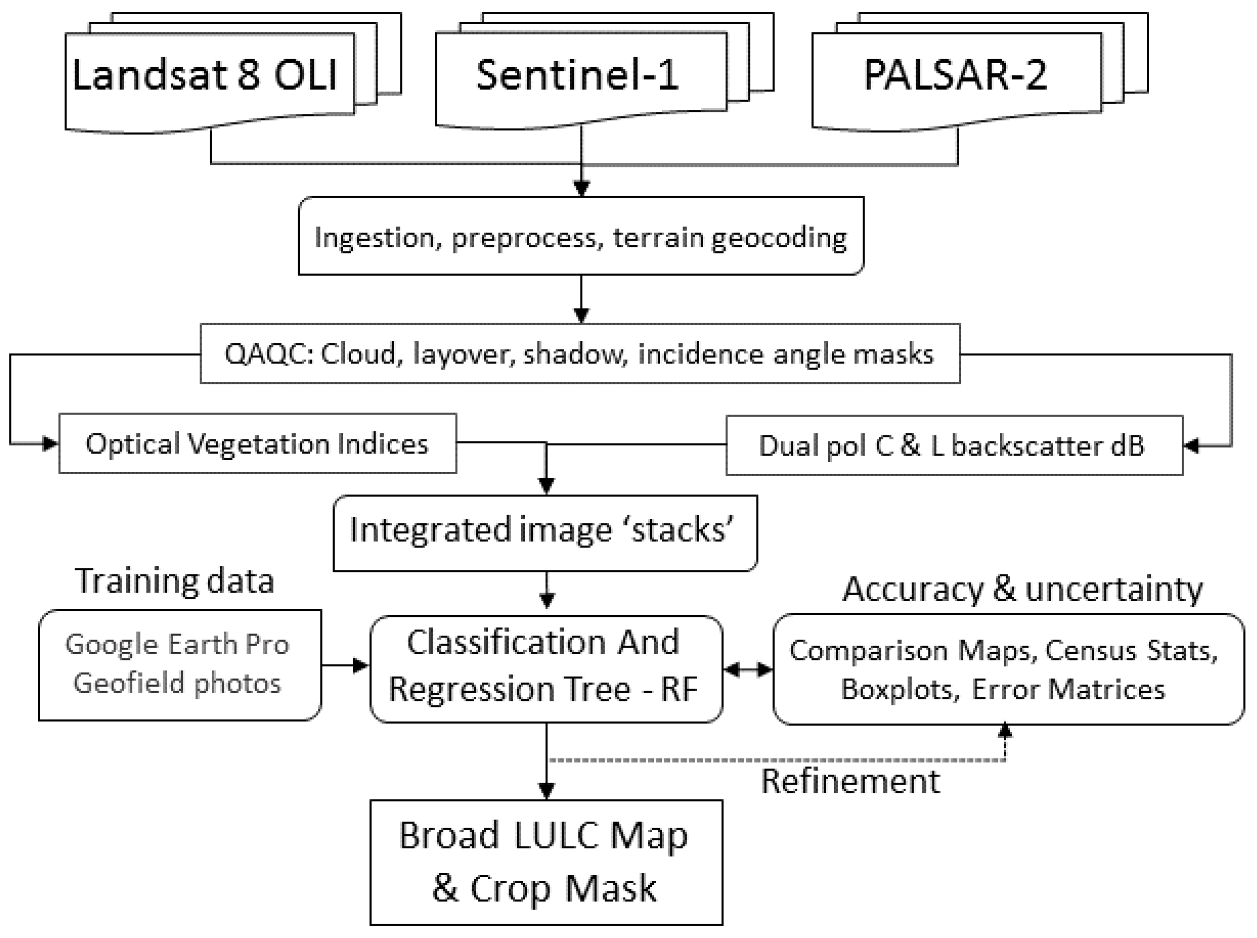
2. Materials and Methods
2.1. Study Areas
Myanmar
2.2. Data Processing
2.2.1. Landsat-8 OLI
2.2.2. PALSAR-2
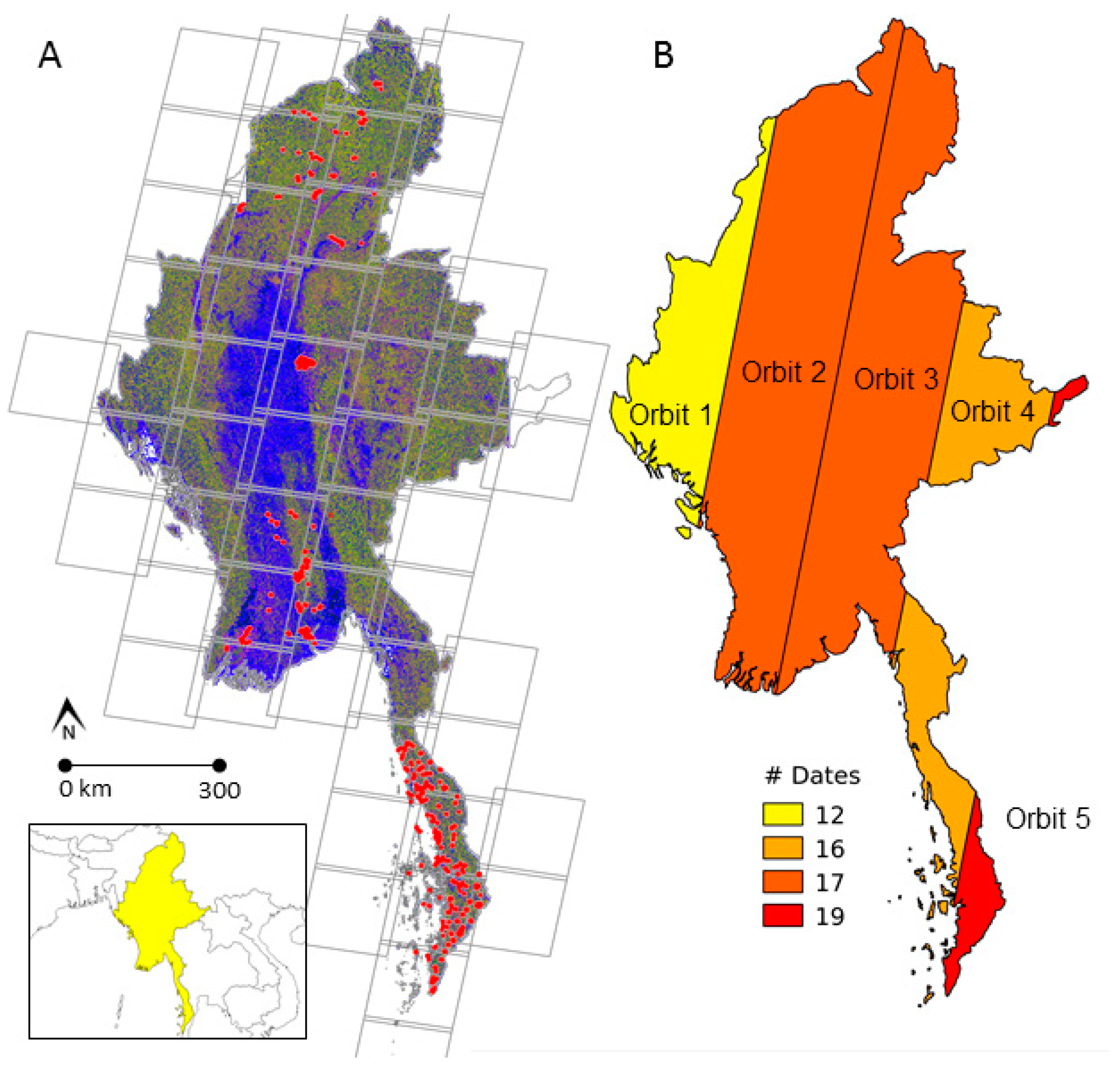
2.2.3. Sentinel-1
2.3. Mapping Approach
2.3.1. Land Use Land Cover Mapping
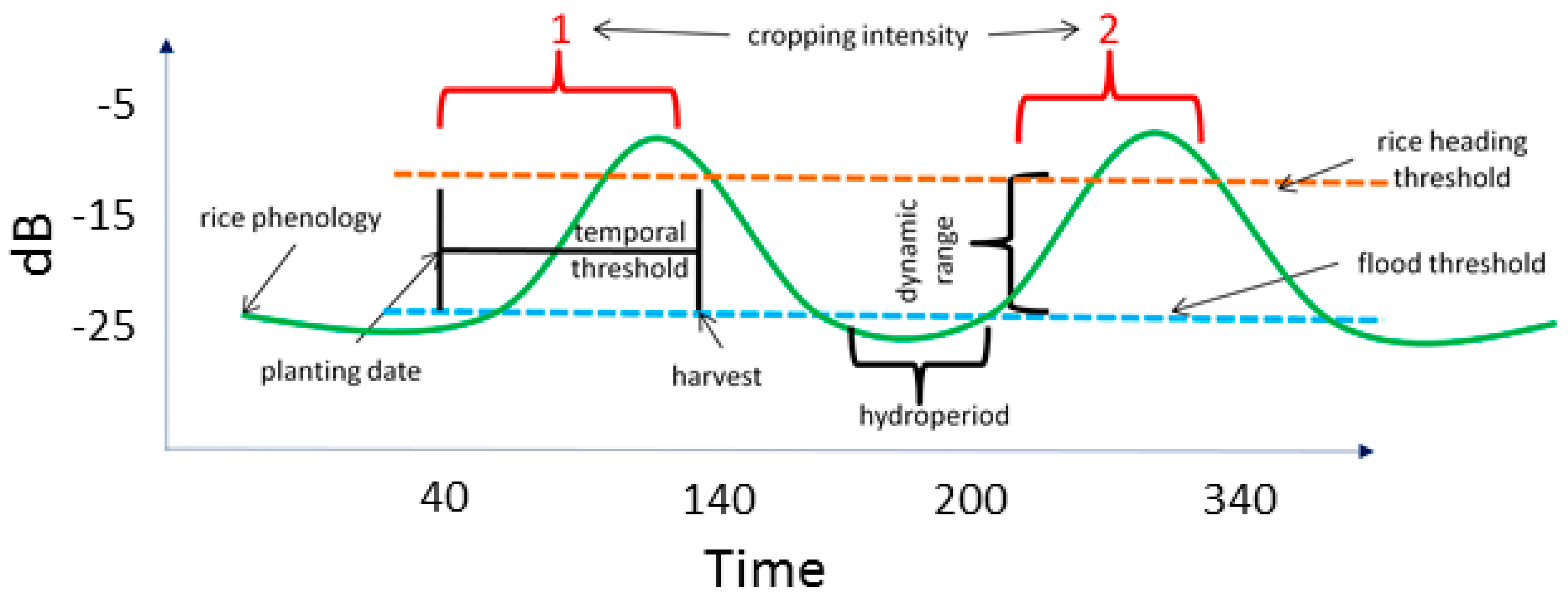
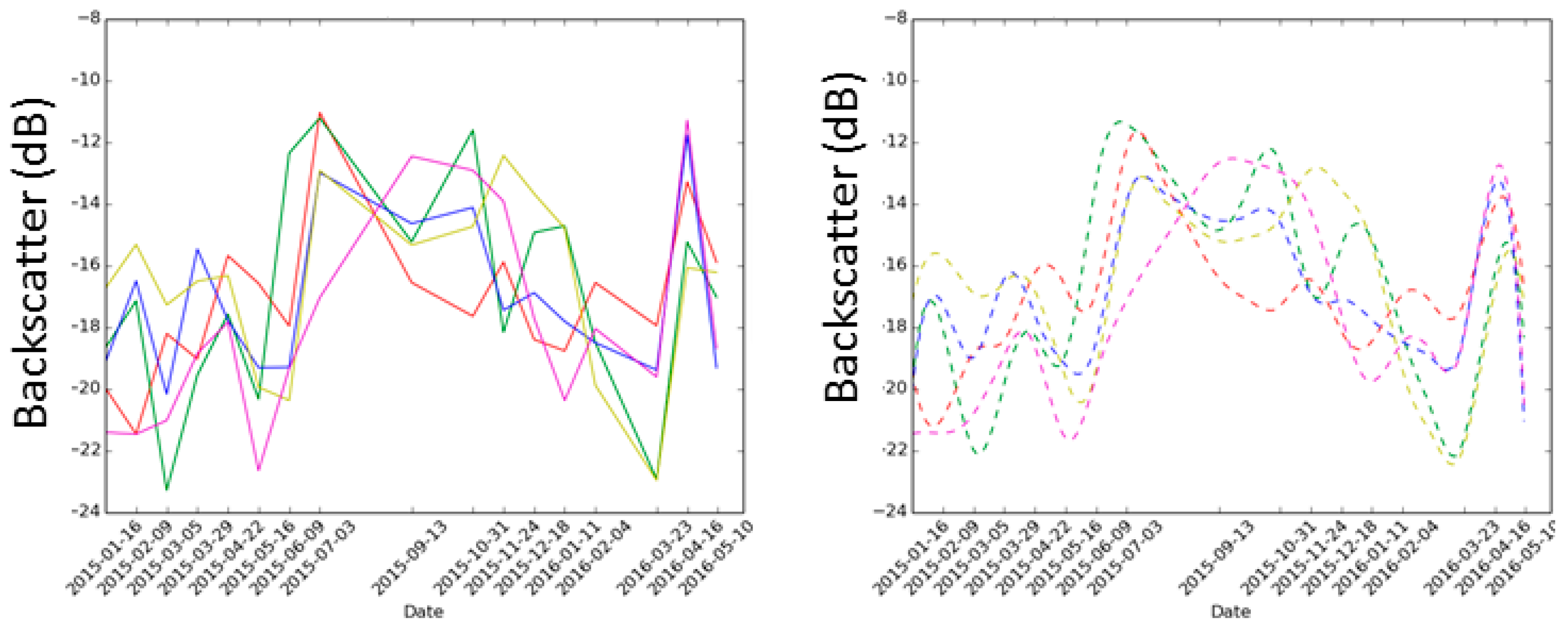
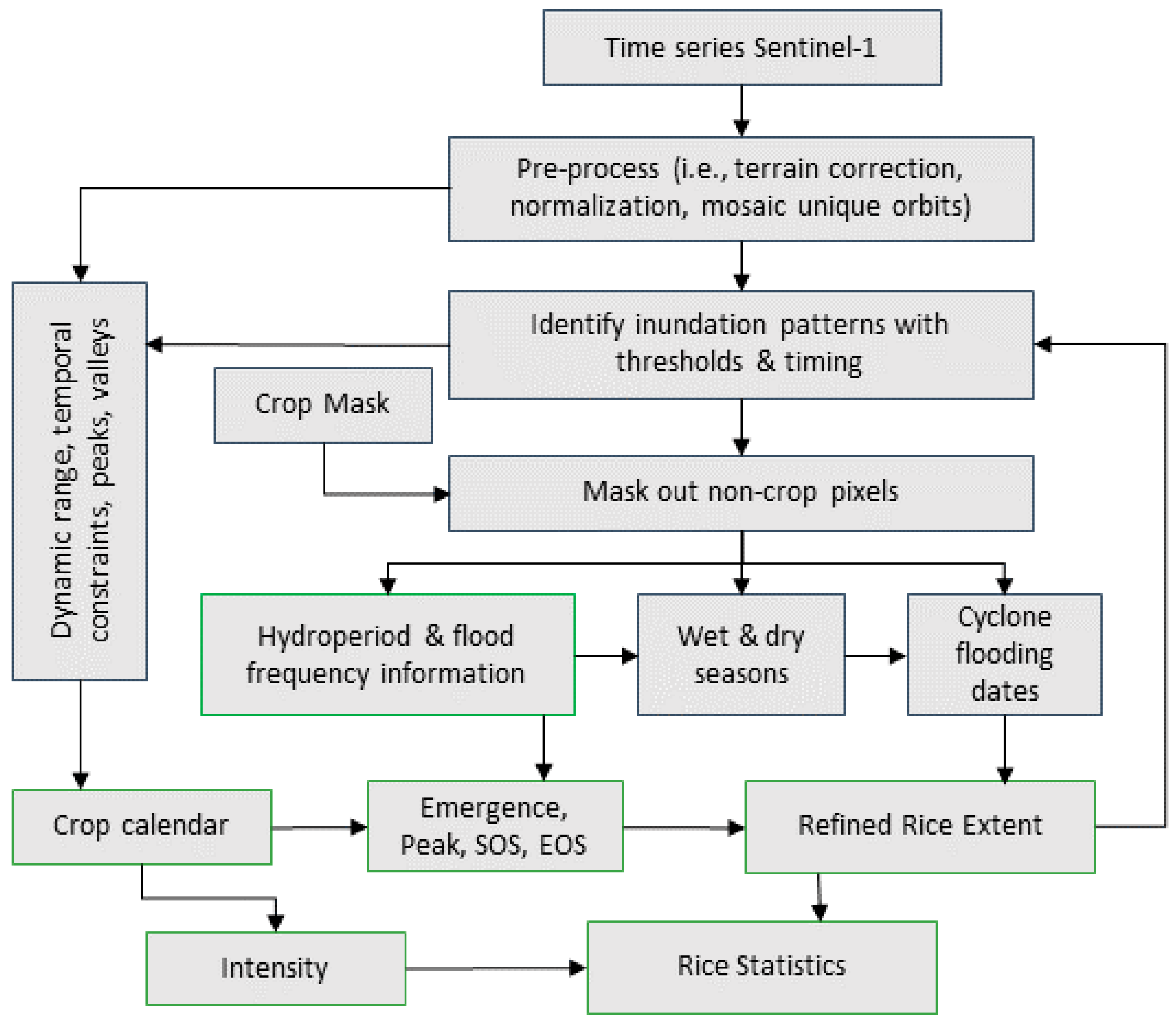
2.3.2. Time Series Analysis
3. Results and Discussion
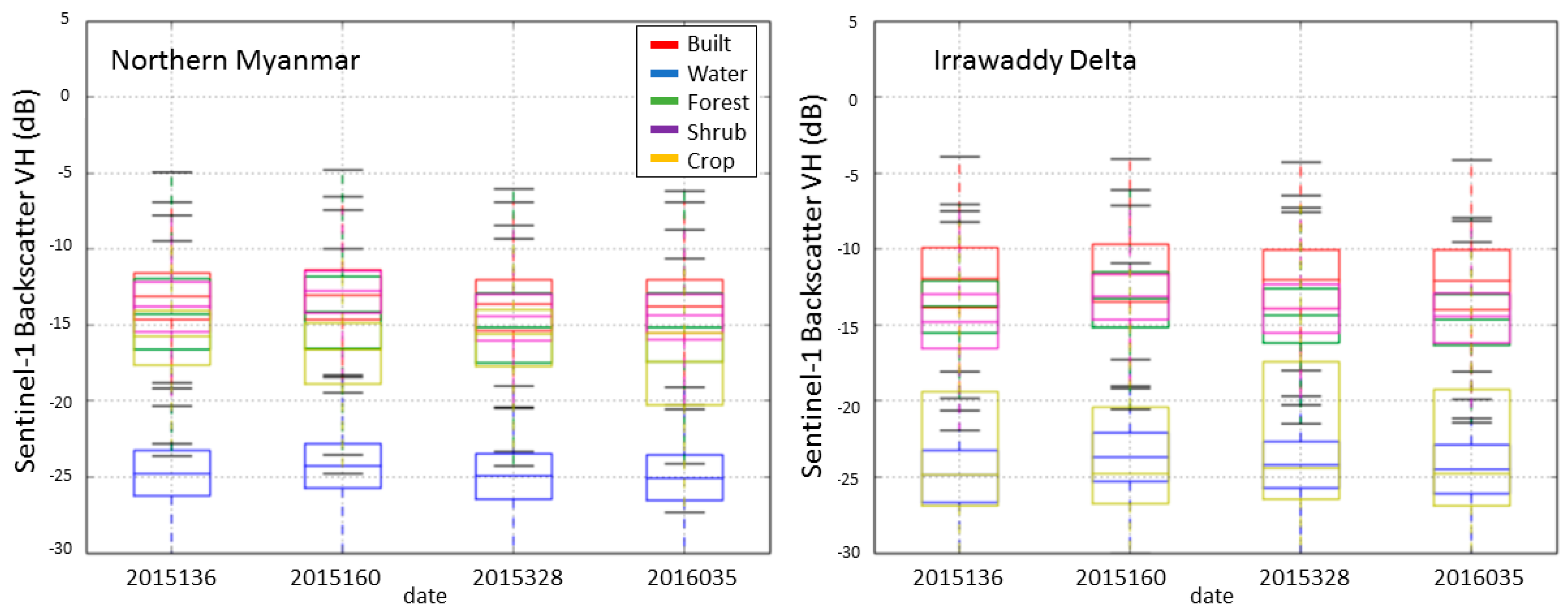
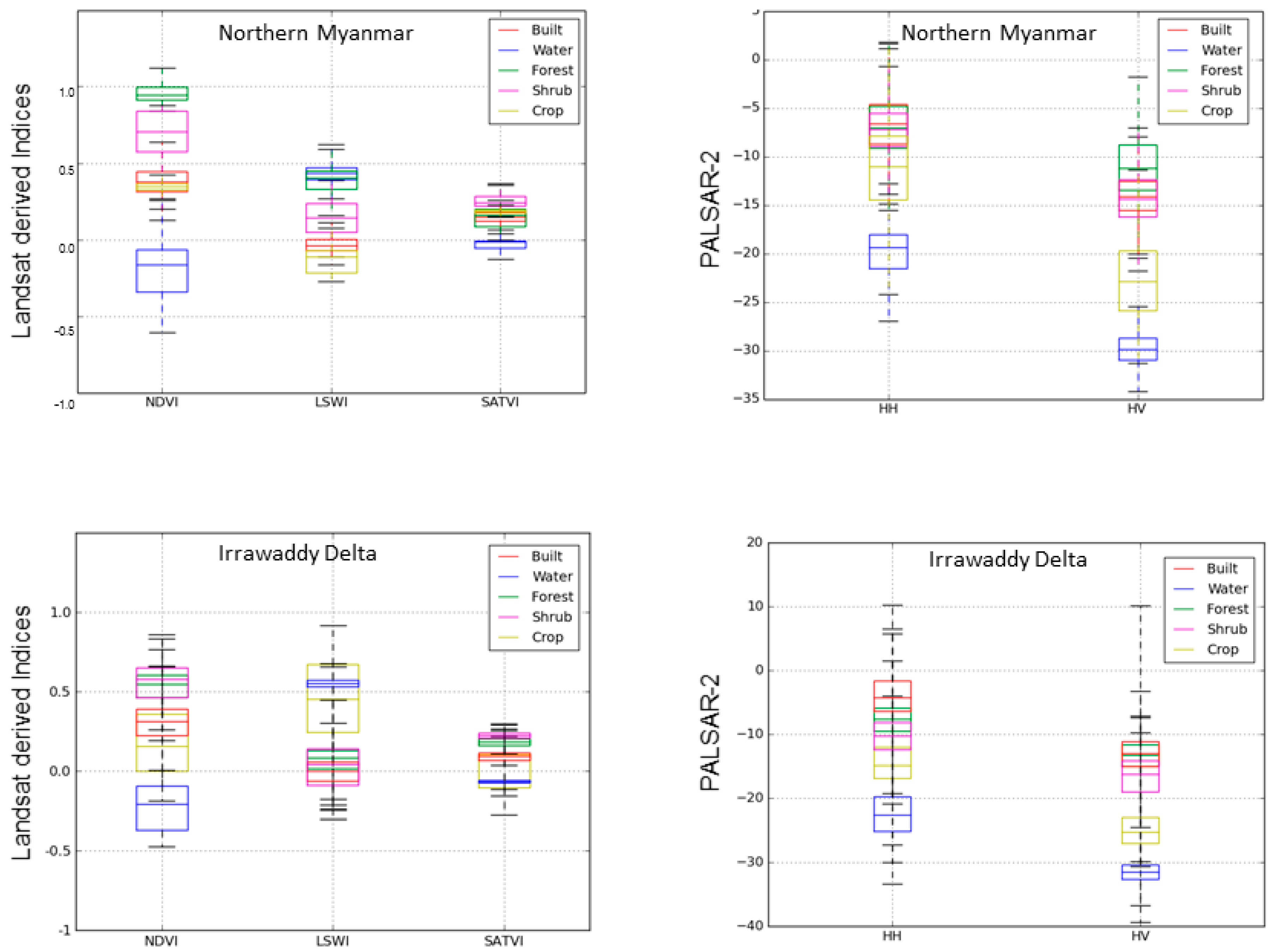
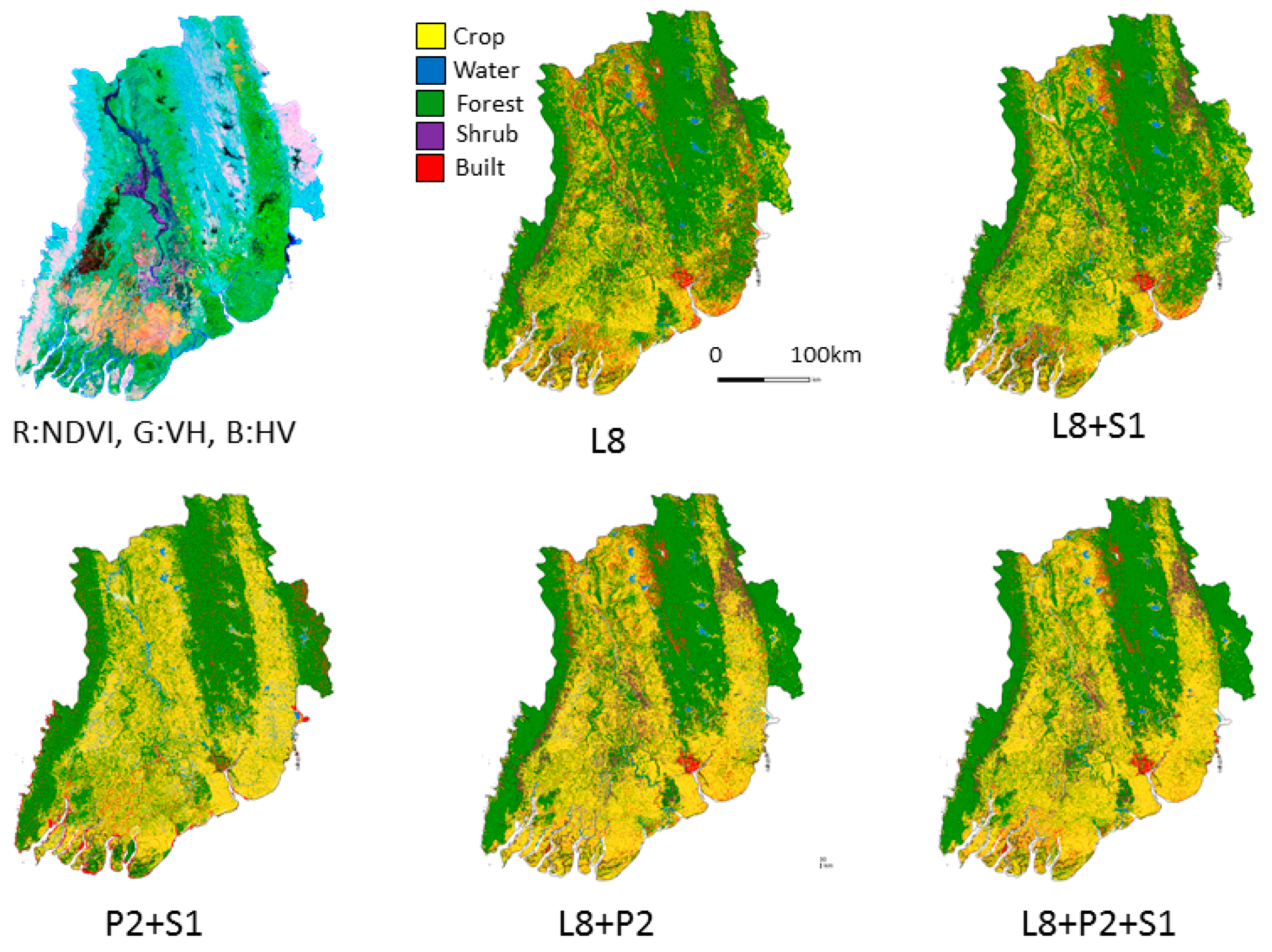
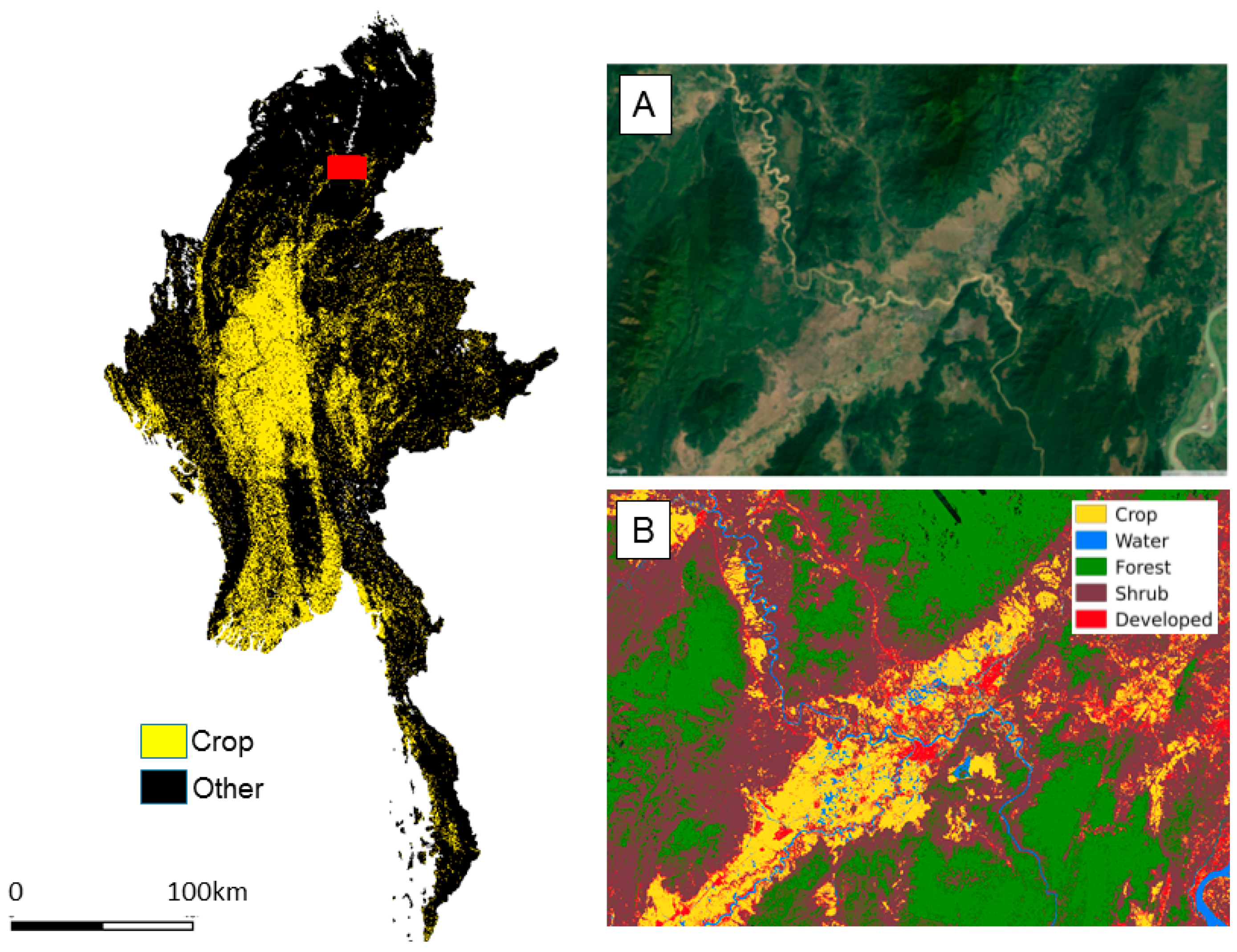
3.1. Mapping Land Cover Land Use
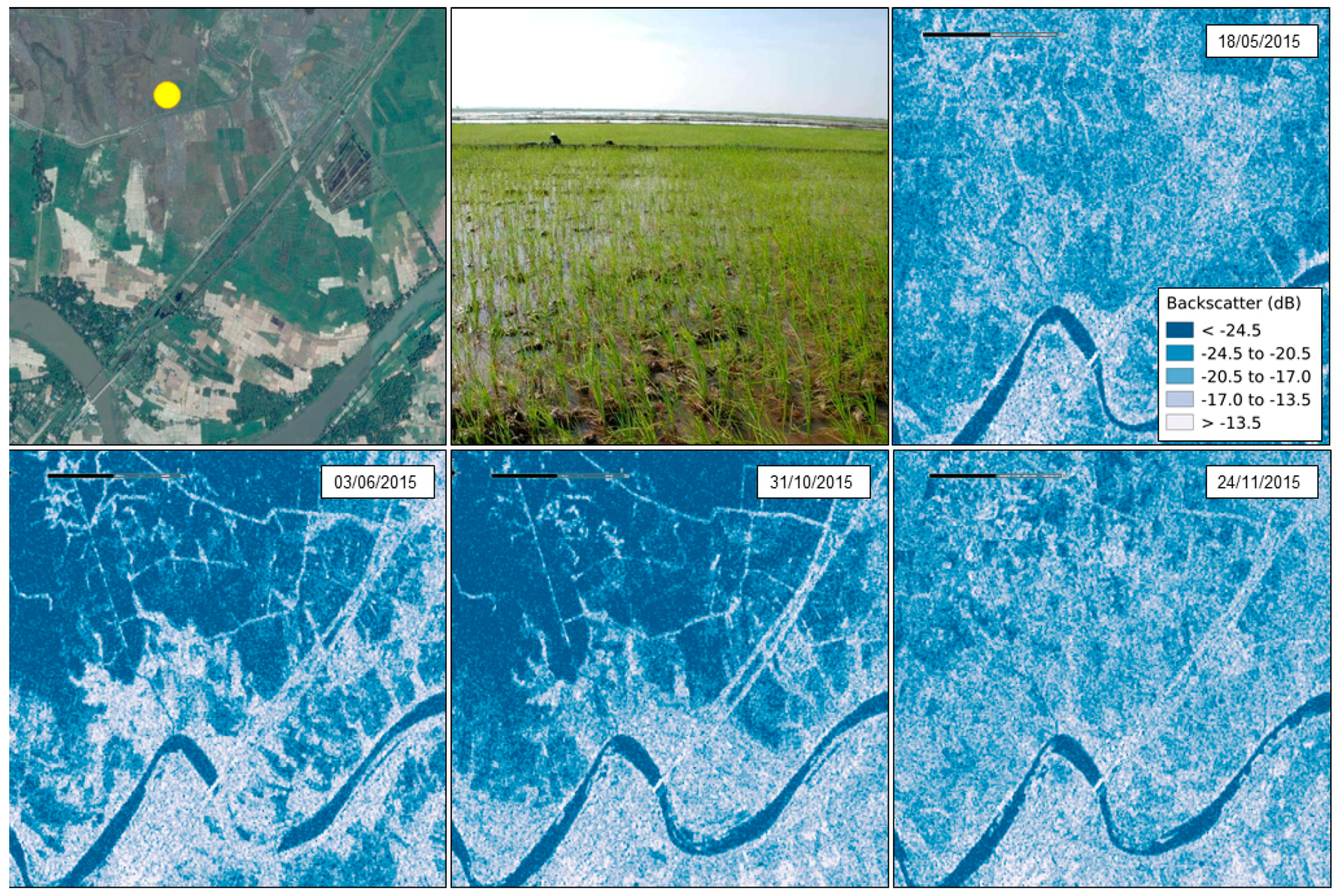
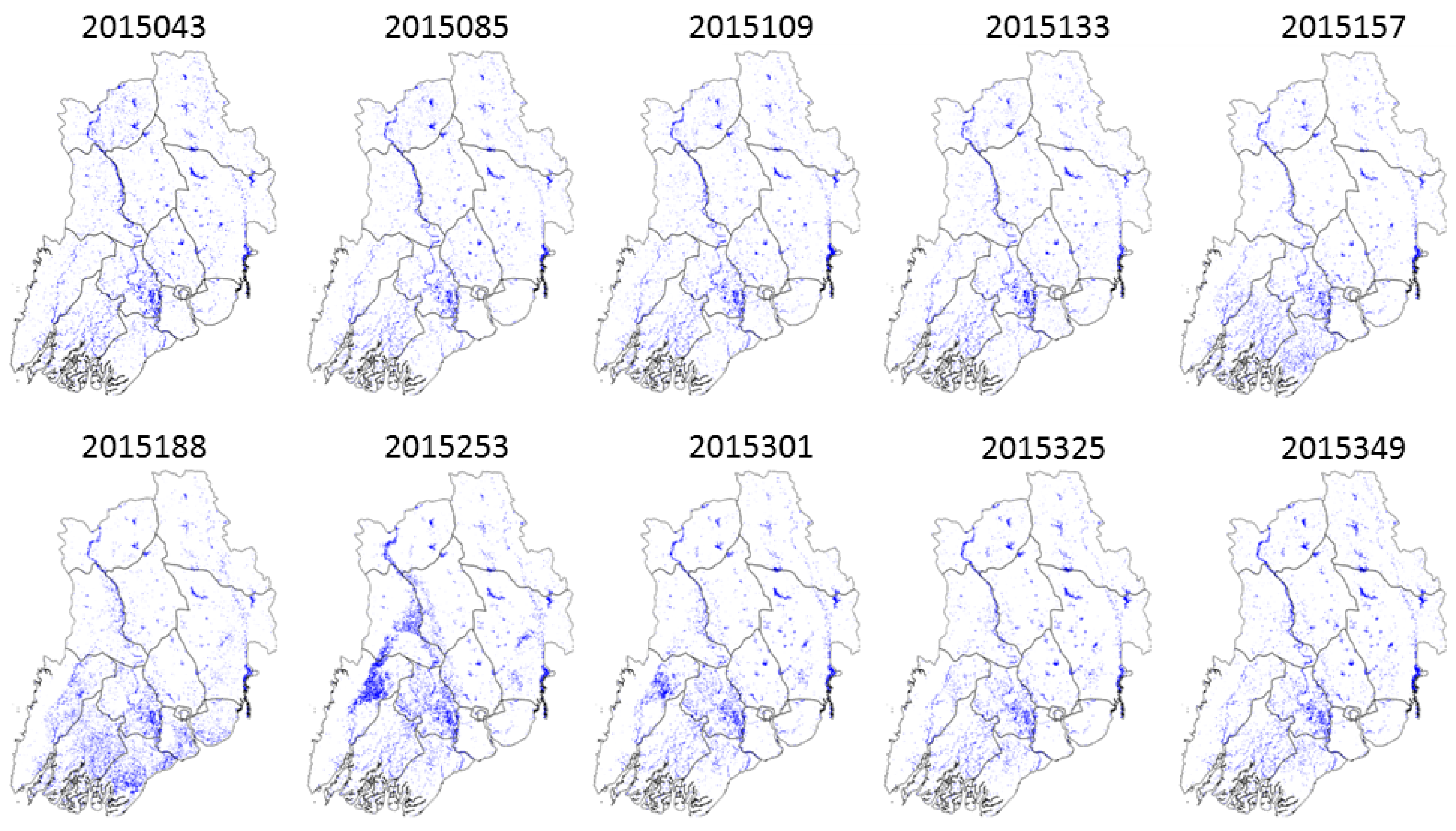
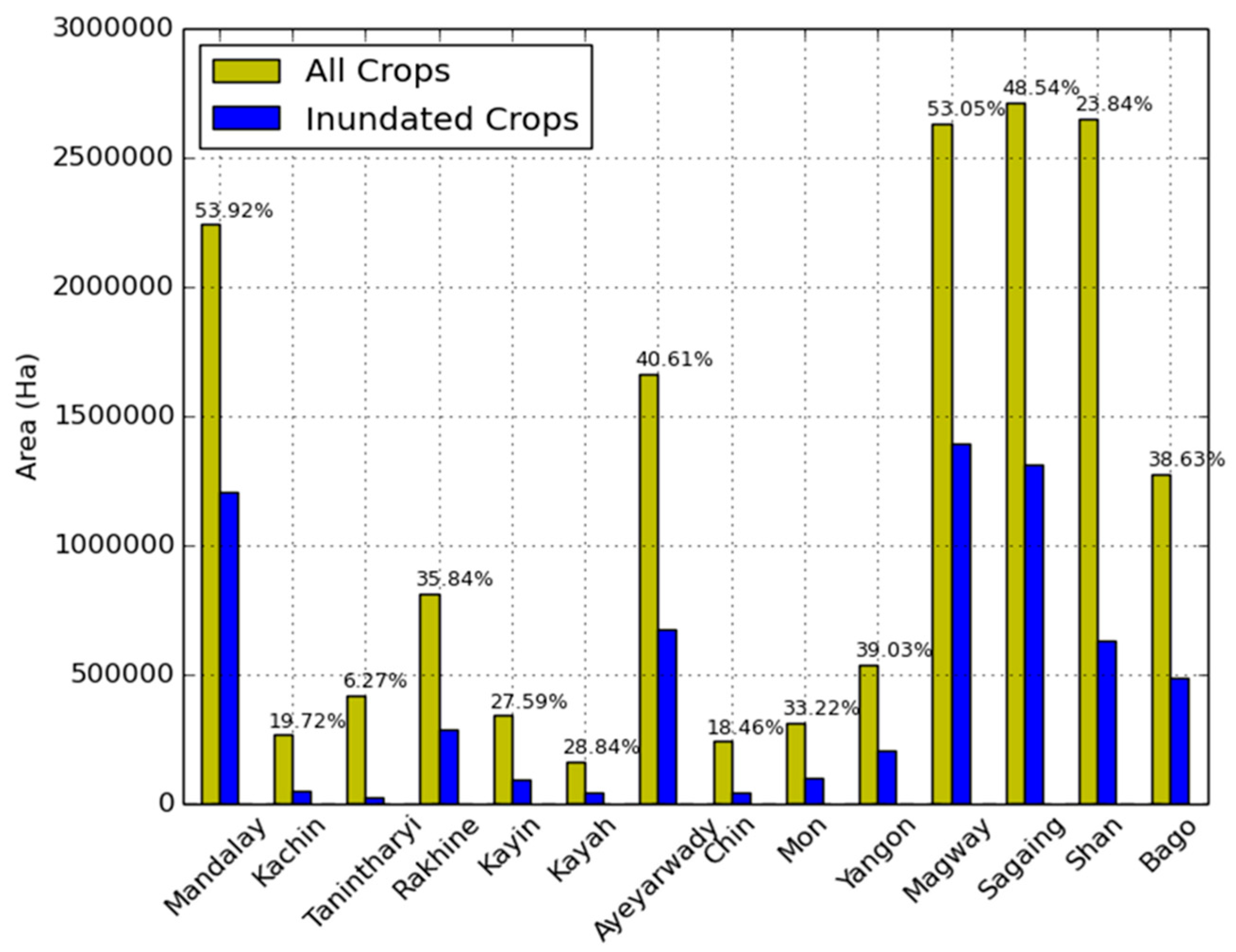
3.2. Mapping Inundation and Refining Rice Extent
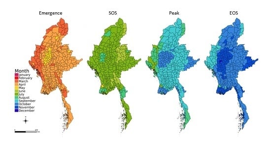
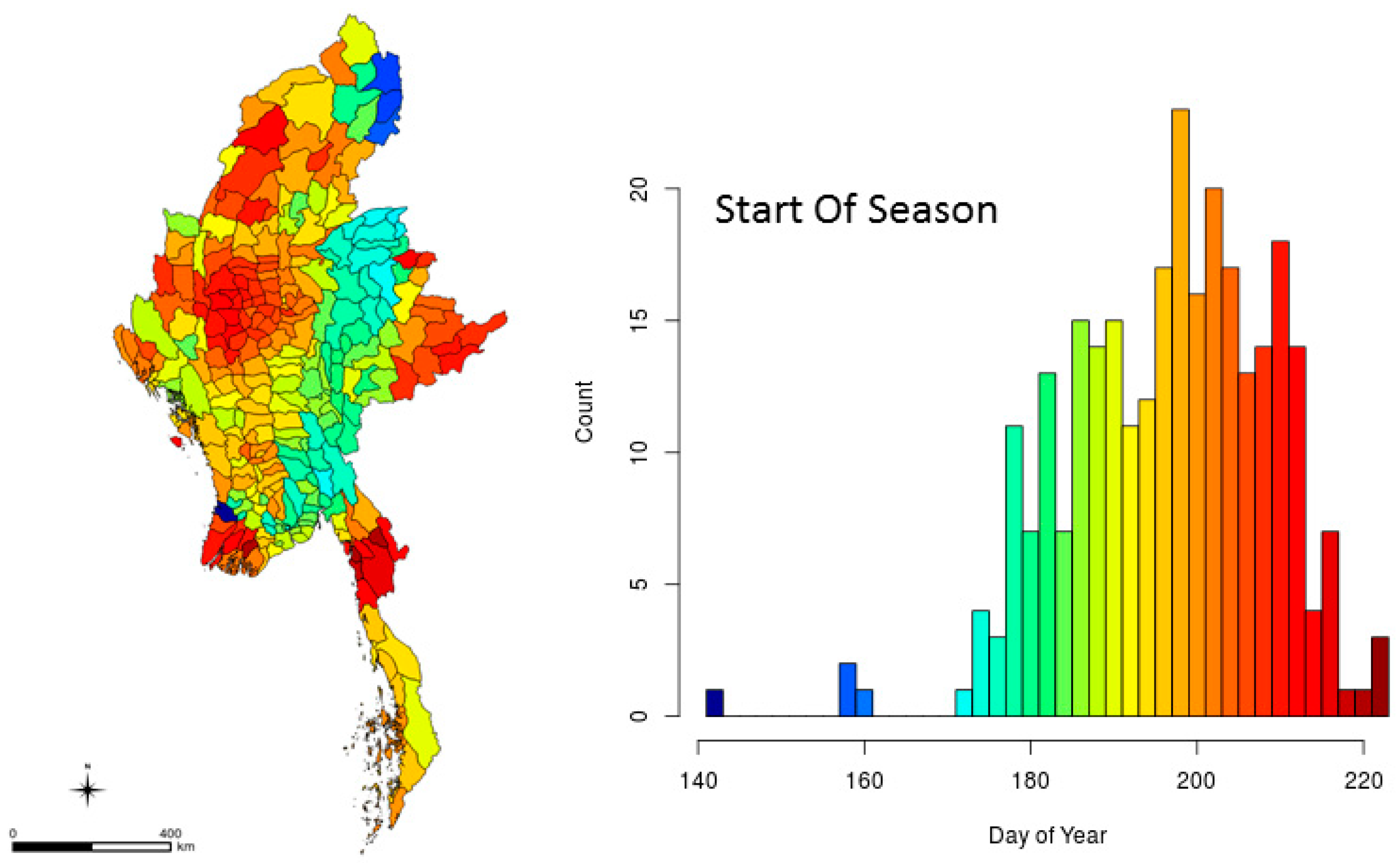
3.3. Mapping Crop Calendar and Intensity
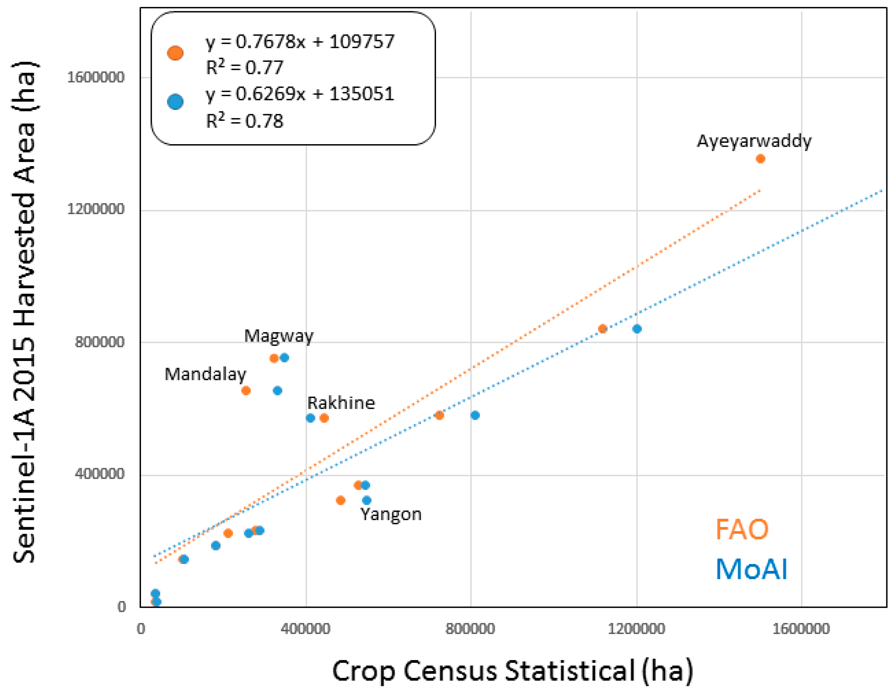
3.4. Comparison and Production Assessment
4. Conclusions
Acknowledgments
Author Contributions
Conflicts of Interest
References
- Food and Agriculture Organization of the United Nations. Available online: http://www.fao.org/home/en (accessed on 15 September 2016).
- Becker-Reshef, I.; Justice, C.; Sullivan, M.; Vermote, E.; Tucker, C.; Anyamba, A.; Small, J.; Pak, E.; Masuoka, E.; Schmaltz, J.; et al. Monitoring Global Croplands with Coarse Resolution Earth Observations: The Global Agriculture Monitoring (GLAM) Project. Remote Sens. 2010, 2, 1589–1609. [Google Scholar] [CrossRef]
- Whitcraft, A.K.; Becker-Reshef, I.; Justice, C.O. A Framework for Defining Spatially Explicit Earth Observation Requirements for a Global Agricultural Monitoring Initiative (GEOGLAM). Remote Sens. 2015, 7, 1461–1481. [Google Scholar] [CrossRef]
- Xiao, X.M.; Boles, S.; Liu, J.Y.; Zhuang, D.F.; Frolking, S.; Li, C. Mapping paddy rice agriculture in southern China using multi-temporal MODIS images. Remote Sens. Environ. 2005, 95, 480–492. [Google Scholar] [CrossRef]
- Sakamoto, T.; Yokozawa, M.; Toritani, H.; Shibayama, M.; Ishitsuka, N.; Ohno, H. Spatio–temporal distribution of rice phenology and cropping systems in the Mekong Delta with special reference to the seasonal water flow of the Mekong and Bassac rivers. Remote Sens. Environ. 2006, 100, 1–16. [Google Scholar] [CrossRef]
- Gumma, M.K.; Nelson, A.; Thenkabail, P.S.; Singh, A.N. Mapping rice areas in South Asia using MODIS multi temporal data. J. Appl. Remote Sens. 2011, 5, 053547. [Google Scholar] [CrossRef]
- Torbick, N.; Salas, W.A.; Hagen, S.; Xiao, X. Mapping rice agriculture in the Sacramento Valley, USA with multitemporal PALSAR and MODIS imagery. IEEE J. Sel. Top. Remote Sens. 2010, 4, 451–457. [Google Scholar] [CrossRef]
- Torbick, N.; Salas, W.; Xiao, X.; Ingraham, P.; Fearon, M.; Biradar, C.; Zhao, D.; Liu, Y.; Li, P.; Zhao, Y. Integrating SAR and optical imagery for regional mapping of paddy rice attributes in the Poyang Lake Watershed, China. Can. J. Remote Sens. 2011, 37, 17–26. [Google Scholar] [CrossRef]
- Clauss, K.; Yan, H.; Kuenzer, C. Mapping Paddy Rice in China in 2002, 2005, 2010 and 2014 with MODIS Time Series. Remote Sens. 2016, 8, 434. [Google Scholar] [CrossRef]
- Guan, X.; Huang, C.; Liu, G.; Meng, X.; Liu, Q. Mapping Rice Cropping Systems in Vietnam Using an NDVI-Based Time-Series Similarity Measurement Based on DTW Distance. Remote Sens. 2016, 8, 19. [Google Scholar] [CrossRef]
- Biradar, C.M.; Xiao, X. Quantifying the area and spatial distribution of double- and triple-cropping croplands in India with multi-temporal MODIS imagery in 2005. Int. J. Remote Sens. 2011, 32, 367–386. [Google Scholar] [CrossRef]
- Xiao, X.; Boles, S.; Frolking, S.; Li, C.; Babu, J.Y.; Salas, W.; Moore, B., III. Mapping paddy rice agriculture in South and Southeast Asia using multi-temporal MODIS images. Remote Sens. Environ. 2006, 100, 95–113. [Google Scholar] [CrossRef]
- Thenkabail, P.S.; Biradar, C.M.; Noojipady, P.; Dheeravath, V.; Li, Y.J.; Velpuri, M.; Gumma, M.; Gangalakunta, O.R.P.; Turral, H.; Cai, X.L.; et al. Global irrigated area map (GIAM), derived from remote sensing, for the end of the last millennium. Int. J. Remote Sens. 2009, 30, 3679–3733. [Google Scholar] [CrossRef]
- Gumma, M.K.; Thenkabail, P.S.; Maunahan, A.; Islam, S.; Nelson, A. Mapping seasonal rice cropland extent and area in the high cropping intensity environment of Bangladesh using MODIS 500 m data for the year 2010. ISPRS J. Photogramm. 2014, 91, 98–113. [Google Scholar] [CrossRef]
- Rojas, O.; Vrieling, A.; Rembold, F. Assessing drought probability for agricultureal areas in Africa with coarse resolution remote sensing imagery. Remote Sens. Environ. 2011, 115, 343–352. [Google Scholar] [CrossRef]
- Torbick, N.; Salas, W. Mapping agricultural wetlands in the Sacramento Valley, USA with satellite remote sensing. Wetl. Ecol. Manag. 2014, 23, 79–94. [Google Scholar] [CrossRef]
- Dong, J.; Xiao, X.; Kou, W.; Qin, Y.; Zhang, G.; Li, L.; Jin, C.; Zhou, Y.; Wang, J.; Biradar, C.; et al. Tracking the dynamics of paddy rice planting area in 1986–2010 through time series Landsat images and phenology-based algorithms. Remote Sens. Environ. 2015, 160, 99–113. [Google Scholar] [CrossRef]
- Zhou, Y.; Xiao, X.; Qin, Y.; Dong, J.; Zhang, G.; Kou, W.; Jin, C.; Wang, J.; Li, X. Mapping paddy rice planting area in rice-wetland coexistent areas through analysis of Landsat 8 OLI and MODIS images. Int. J. Appl. Earth Obs. 2016, 46, 1–12. [Google Scholar] [CrossRef] [PubMed]
- Chen, C.; McNairn, H. A neural network integrated approach for rice crop monitoring. Int. J. Remote Sens. 2006, 27, 1367–1393. [Google Scholar] [CrossRef]
- Inoue, Y.; Kurosu, T.; Mseno, H.; Uratsuka, S.; Kozu, T.; Dabrowska-Zielinska, K.; Qi, J. Season-long daily measurements of multifrequency (Ka, Ku, X, C, and L) and full-polarizaiton backscatter signatures over paddy rice field and their relationship with biological variables. Remote Sens. Environ. 2002, 81, 194–204. [Google Scholar] [CrossRef]
- Le Toan, T.; Ribbes, F.; Wang, L.F.; Floury, N.; Ding, K.H.; Kong, J.A.; Fujita, M. Rice Crop Mapping and Monitoring Using ERS-1 Data Based on Experiment and Modeling Results. IEEE Trans. Geosci. Remote 1997, 35, 41–56. [Google Scholar] [CrossRef]
- Ribbes, F.; Le Toan, T. Rice parameter retrieval and yield prediction using radarsat data. In Towards Digital Earth; International Symposium in Digital Earth: Toulouse, France, 1999. [Google Scholar]
- Bouvet, A.; Le Toan, T.; Lam-Dao, N. Monitoring of the rice cropping system in the Mekong Delta using ENVISAT/ASAR dual polarization data. IEEE Trans. Geosci. Remote 2009, 47, 517–526. [Google Scholar] [CrossRef] [Green Version]
- Kuenzer, C.; Knauer, K. Remote sensing of rice crop areas. Int. J. Remote Sens. 2013, 34, 2101–2139. [Google Scholar] [CrossRef]
- Inoue, Y.; Sakaiya, E.; Wang, C. Capability of C-band backscattering coefficients from high-resolution satellite SAR sensors to assess biophysical variables in paddy rice. Remote Sens. Environ. 2014, 140, 257–266. [Google Scholar] [CrossRef]
- Nelson, A.; Setiyono, T.; Rala, A.B.; Quicho, E.D.; Raviz, J.V.; Abonete, P.J.; Maunahan, A.A.; Garcia, C.A.; Bhatti, H.Z.M.; Villano, L.S.; et al. Towards an Operational SAR-Based Rice Monitoring System in Asia: Examples from 13 Demonstration Sites across Asia in the RIICE Project. Remote Sens. 2014, 6, 10773–10812. [Google Scholar] [CrossRef]
- Torres, R.; Snoeij, P.; Geudtner, D.; Bibby, D.; Davidson, M.; Attema, E.; Potin, P.; Rommen, B.; Floury, N.; Brown, M.; et al. GMES Sentinel-1 mission. Remote Sens. Environ. 2012, 120, 9–24. [Google Scholar] [CrossRef]
- Torbick, N.; Salas, W.; Chowdhury, D.; Ingraham, P. Mapping rice greenhouse gas emissions in the Red River Delta Vietnam. Carb. Manag. 2017, in press. [Google Scholar]
- United States Department of Agriculture Foreign Agricultural Service. Available online: http://www.fas.usda.gov (accessed on 9 September 2016).
- Roy, D.P.; Wulder, M.A.; Loveland, T.R.; Woodcock, C.E.; Allen, R.G.; Anderson, M.C.; Scambos, T.A. Landsat-8: Science and product vision for terrestrial global change research. Remote Sens. Environ. 2014, 145, 154–172. [Google Scholar] [CrossRef]
- Vermote, E.; Justice, C.; Claverie, M.; Franch, B. Preliminary analysis of the performance of the Landsat 8/OLI land surface reflectance product. Remote Sens. Environ. 2016, 185, 46–56. [Google Scholar] [CrossRef]
- Masek, J.G.; Vermote, E.F.; Saleous, N.E.; Wolfe, R.; Hall, F.G.; Huemmrich, K.F.; Gao, F.; Kutler, J.; Lim, T.K. A Landsat surface reflectance dataset for North America, 1990–2000. IEEE Geosci. Remote Sens. Soc. 2006, 3, 68–72. [Google Scholar] [CrossRef]
- Vermote, E.F.; El Saleous, N.; Justice, C.O.; Kaufman, Y.J.; Privette, J.L.; Remer, L.; Roger, J.C.; Tanré, D. Atmospheric correction of visible to middle-infrared EOS-MODIS data over land surfaces: Background, operational algorithm and validation. J. Geophys. Res.-Atmos. 1997, 102, 17131–17141. [Google Scholar] [CrossRef]
- Zhu, Z.; Woodcock, C.E. Object-based cloud and cloud shadow detection in Landsat imagery. Remote Sens. Environ. 2012, 118, 83–94. [Google Scholar] [CrossRef]
- Vermote, E.F.; Kotchenova, S. Atmospheric correction for the monitoring of land surfaces. J. Geophys. Res.-Atmos. 2008, 113. [Google Scholar] [CrossRef]
- Irish, R.R.; Barker, J.L.; Goward, S.N.; Arvidson, T. Characterization of the Landsat 7 ETM+ automated cloud cover assessment (ACCA) algorithm. Photogramm. Eng. Remote Sens. 2006, 72, 1179–1188. [Google Scholar] [CrossRef]
- Rouse, J.W., Jr.; Haas, R.H.; Schell, J.A.; Deering, D.W. Monitoring vegetation systems in the Great Plains with ERTS. In Proceedings of the Third ERTS Symposium, Washington, DC, USA, 10 December 1974; Freden, S.C., Mercanti, E.P., Becker, M.A., Eds.; pp. 309–317.
- Tucker, C.J. Red and photographic infrared linear combinations for monitoring vegetation. Remote Sens. Environ. 1979, 8, 127–150. [Google Scholar] [CrossRef]
- Xiao, X.; Boles, S.; Liu, J.; Zhuang, D.; Liu, M. Characterization of forest types in Northeastern China, using multi-temporal SPOT-4 VEGETATION sensor data. Remote Sens. Environ. 2002, 82, 335–348. [Google Scholar] [CrossRef]
- Hagen, S.; Heilman, P.; Marsett, R.; Torbick, N.; Salas, W.; van Ravensway, J.; Qi, J. Mapping total vegetation cover across western rangelands with MODIS data. Rangel. Ecol. Manag. 2012, 65, 456–467. [Google Scholar] [CrossRef]
- Xiao, X.; Dorovskoy, P.; Biradar, C.; Bridge, E. A library of georeferenced photos from the field. EOS Earth Space Sci. 2011, 92, 453–454. [Google Scholar] [CrossRef]
- Torbick, N.; Ledoux, L.; Salas, W.; Zhao, M. Regional Mapping of Plantation Extent Using Multisensor Imagery. Remote Sens. 2016, 8, 236. [Google Scholar] [CrossRef]
- Breiman, L. Random Forests. Mach. Learn. 2001, 45, 5–32. [Google Scholar] [CrossRef]
- Lawrence, R.L.; Wood, S.D.; Sheley, R.L. Mapping invasive plants using hyperspectral imagery and Breiman cutler classifications (randomForest). Remote Sens. Environ. 2006, 100, 356–362. [Google Scholar] [CrossRef]
- Watts, J.D.; Lawrence, R.L.; Miller, P.R.; Montagne, C. Monitoring of cropland practices for carbon sequestration purposes in north central Montana by Landsat remote sensing. Remote Sens. Environ. 2009, 113, 1843–1852. [Google Scholar] [CrossRef]
- Schultz, B.; Immitzer, M.; Formaggio, A.R.; Sanches, I.D.A.; Luiz, A.J.B.; Atzberger, C. Self-guided segmentation and classification of multi-temporal Landsat 8 images for crop type mapping in southwestern Brazil. Remote Sens. 2015, 7, 14482–14508. [Google Scholar] [CrossRef]
- Whitcomb, J.; Moghaddam, M.; McDonlad, K.; Kellndorfer, J.; Podest, E. Mapping vegetated wetlands of Alaska using L-band radar satellite imagery. Can. J. Remote Sens. 2009, 35, 54–72. [Google Scholar] [CrossRef]
- Torbick, N.; Persson, A.; Olefeldt, D.; Frolking, S.; Salas, W.; Hagen, S.; Crill, P.; Li, C. High resolution mapping of peatland hydroperiod at a high-latitude Swedish mire. Remote Sens. 2012, 4, 1974–1994. [Google Scholar] [CrossRef]
- Wilkes, P.; Jones, S.D.; Suarez, L.; Mellor, A.; Woodgate, W.; Soto-Berelov, M.; Haywood, A.; Skidmore, A.K. Mapping forest canopy height over large areas by upscaling ALS estimates with freely available satellite data. Remote Sens. 2015, 7, 12563–12587. [Google Scholar] [CrossRef]
- Song, W.; Dolon, J.M.; Cline, D.; Xiong, G. Leanring-based algal bloom event recognition for oceanographic decision support system using remote sensing data. Remote Sens. 2015, 7, 13564–13585. [Google Scholar] [CrossRef]
- Torbick, N.; Corbiere, M. Mapping urban sprawl and impervious surfaces in the northeast United States for the past four decades. GISci Remote Sens. 2015, 52, 746–764. [Google Scholar] [CrossRef]
- Karlson, M.; Ostwald, M.; Reese, H.; Sanou, J.; Tankoano, B.; Mattsson, E. Mapping tree canopy cover and aboveground biomass in Sudano-Sahelian woodlands using Landsat 8 and random forest. Remote Sens. 2015, 7, 10017–10041. [Google Scholar] [CrossRef]
- Nguyen, D.B.; Gruber, A.; Wagner, W. Mapping rice extent and cropping scheme in the Mekong Delta using Sentinel-1A data. Remote Sens. Lett. 2016, 7, 1209–1218. [Google Scholar] [CrossRef]
- Savitzky, A.; Golay, M.J.E. Smoothing and Differentiation of Data by Simplified Least Squares Procedures. Anal. Chem. 1964, 36, 1627–1639. [Google Scholar] [CrossRef]
- Whittaker, E.T.; Robinson, G. The Calculus of Observations. Trans. Fac. Act. 1924, 10, 1924–1925. [Google Scholar]
- Atzberger, C.; Eilers, P.H.C. A time series for monitoring vegetation activity and phenology at 10-daily time steps covering large parts of South America. Int. J. Dig. Earth 2011, 4, 365–386. [Google Scholar] [CrossRef]
- Atkinson, P.M.; Jeganathan, C.; Dash, J.; Atzberger, C. Inter-comparison of four models for smoothing satellite sensor time-series data to estimate vegetation phenology. Remote Sens. Environ. 2012, 123, 400–417. [Google Scholar] [CrossRef]
- Eilers, P.H.C. A Perfect Smoother. Anal. Chem. 2003, 75, 3631–3636. [Google Scholar] [CrossRef] [PubMed]
- Inglada, J.; Vincent, A.; Arias, M.; Marais-Sicre, C. Improved Early Crop Type Identification By Joint Use of High Temporal Resolution SAR And Optical Image Time Series. Remote Sens. 2016, 8, 362. [Google Scholar] [CrossRef]


| J | F | M | A | M | J | J | A | S | O | N | D | |
|---|---|---|---|---|---|---|---|---|---|---|---|---|
| Rice (main; wet season) | ||||||||||||
| Rice (second) | ||||||||||||
| Sowing | ||||||||||||
| Growing | ||||||||||||
| Harvest |
| Class | # of Polygons | # of Pixels | Min Patch (Ha) | Max Patch (Ha) |
|---|---|---|---|---|
| Crop | 100 | 72,686 | 1.36 | 695.66 |
| Water | 92 | 76,888 | 0.62 | 1125.40 |
| Forest | 100 | 903,064 | 1.31 | 4862.90 |
| Shrub | 73 | 14,900 | 0.16 | 207.34 |
| Built | 94 | 68,822 | 2.97 | 325.34 |
| Tanintharyi | Crop | Water | Forest | Shrub | Developed | |
| Crop | 35,962 | 1 | 1 | 0 | 23 | |
| Water | 0 | 27,265 | 0 | 0 | 1 | |
| Forest | 5 | 2 | 794,587 | 24 | 0 | |
| Shrub | 0 | 0 | 122 | 11,124 | 0 | |
| Developed | 43 | 9 | 4 | 0 | 36,903 |
| Landsat-8 | 0.94 |
| Landsat-8, PALSAR-2 | 0.95 |
| Landsat-8, Sentinel-1 | 0.94 |
| Sentinel-1, PALSAR-2 | 0.71 |
| Landsat-8, Sentinel-1, PALSAR-2 | 0.95 |
© 2017 by the authors. Licensee MDPI, Basel, Switzerland. This article is an open access article distributed under the terms and conditions of the Creative Commons Attribution (CC BY) license ( http://creativecommons.org/licenses/by/4.0/).
Share and Cite
Torbick, N.; Chowdhury, D.; Salas, W.; Qi, J. Monitoring Rice Agriculture across Myanmar Using Time Series Sentinel-1 Assisted by Landsat-8 and PALSAR-2. Remote Sens. 2017, 9, 119. https://doi.org/10.3390/rs9020119
Torbick N, Chowdhury D, Salas W, Qi J. Monitoring Rice Agriculture across Myanmar Using Time Series Sentinel-1 Assisted by Landsat-8 and PALSAR-2. Remote Sensing. 2017; 9(2):119. https://doi.org/10.3390/rs9020119
Chicago/Turabian StyleTorbick, Nathan, Diya Chowdhury, William Salas, and Jiaguo Qi. 2017. "Monitoring Rice Agriculture across Myanmar Using Time Series Sentinel-1 Assisted by Landsat-8 and PALSAR-2" Remote Sensing 9, no. 2: 119. https://doi.org/10.3390/rs9020119