Modelling Diverse Soil Attributes with Visible to Longwave Infrared Spectroscopy Using PLSR Employed by an Automatic Modelling Engine

Abstract

The study tested a data mining engine (PARACUDA^®) to predict various soil attributes (BC, CEC, BS, pH, C_org, Pb, Hg, As, Zn and Cu) using reflectance data acquired for both optical and thermal infrared regions. The engine was designed to utilize large data in parallel and automatic processing to build and process hundreds of diverse models in a unified manner while avoiding bias and deviations caused by the operator(s). The system is able to systematically assess the effect of diverse preprocessing techniques; additionally, it analyses other parameters, such as different spectral resolutions and spectral coverages that affect soil properties. Accordingly, the system was used to extract models across both optical and thermal infrared spectral regions, which holds significant chromophores. In total, 2880 models were evaluated where each model was generated with a different preprocessing scheme of the input spectral data. The models were assessed using statistical parameters such as coefficient of determination (R²), square error of prediction (SEP), relative percentage difference (RPD) and by physical explanation (spectral assignments). It was found that the smoothing procedure is the most beneficial preprocessing stage, especially when combined with spectral derivation (1st or 2nd derivatives). Automatically and without the need of an operator, the data mining engine enabled the best prediction models to be found from all the combinations tested. Furthermore, the data mining approach used in this study and its processing scheme proved to be efficient tools for getting a better understanding of the geochemical properties of the samples studied (e.g., mineral associations).

1. Introduction

Soil spectroscopy has proven to be a fast, environmentally-friendly, reproducible, and repeatable analytical technique that has been increasingly used for rapid, non-destructive and cost-effective soil analyses. Spectroscopy, covering the optical (reflected solar radiation) and thermal infrared (earth surface emitted radiation) regions across the 0.4–15 µm spectral range, can be used to determine a wide range of soil properties [1] such as organic carbon (OC) [2], texture [3], cationic exchange capacity (CEC) [4], total phosphorus (P) [5], exchangeable potassium (K) [6], electrical conductivity (EC) [7,8,9], total concentration of potential pollutant metals/metalloids [10] and mineral content [11,12]. Aside from the fundamental interaction of electromagnetic radiation with matter, indirect interaction can be found and provide additional quantitative information of the soil in question [13]. The chemical or physical phenomenon that interacts with electromagnetic radiation is termed a chromophore.

The interaction between matter and electromagnetic radiation has been studied from both the theoretical and practical points of view. The spectral information is represented by a spectrum which consists of visible as well as non-visible information to the naked eye that further, when extracted, can spotlight the material in question in both quantitative and qualitative ways. The previously mentioned spectral regions can be divided into sub-regions: visible (VIS, 0.4–0.7 µm), near infrared (NIR, 0.7–1.0 µm), shortwave infrared (SWIR, 1.0–3.0 µm), mid-wave infrared (MWIR, 3.0–7.0 µm) and longwave infrared (LWIR, 7.0–15 µm).

Analysing the spectral data can yield quantitative information about the material’s chemical composition. This is because the spectral characteristics are correlated with the direct and indirect chromophores across all regions. In the VIS and NIR regions, iron oxides (due to electronic transitions) and organic matter are the main chromophores. Across the SWIR region the main active chromophores are OH in free water and the clay mineral lattice, organic matter, carbonates and salts [13]. In the MWIR and LWIR spectral regions, absorption features, resulting from fundamental molecular vibration modes, show additional information about soil constituents, such as Si-bearing minerals (mainly quartz and clay minerals), carbonates, organic matter and gypsum [1,14].

High-dimensional spectral datasets, which are typically obtained in the solid and liquid phase, are used as inputs for quantitative modelling in spectroscopy. The data mining stage for extracting a valid model requires adequate statistical analysis techniques, which are able to deal with many highly collinear spectral frequencies (predictor variables) from relatively few observations. In this regard, multivariate analysis techniques, such as Multiple Linear Regression (MLR) [15], Principal Component Regression (PCR) and Partial Least Squares Regression (PLSR) analyses [16], are capable of extracting reasonable models with overlapping information. Recently, different approaches have been used for spectroscopic data modelling including the artificial neural network (ANN, [17]), support vector machine regression (SVM, [18]) and random forests (RF) regression [19]; however PLSR is still probably the most widely used analysis technique over all, as it is an adequate technique to handle the difficulties inherited from the interpreted overtones by extracting the response variable relevant information from the spectra, while ignoring redundant information [12,15,20].

Prior to employing statistical modelling to detect the relationship between spectroscopy and the chemical properties of the material, different types of preprocessing techniques can be applied to the input spectral information (e.g., [18,21,22,23]) either to minimize the noise or normalize the input spectroscopic data. Among these methods, the most common are: smoothing techniques, spectral derivatives, transfer to a logarithmic scale or continuum removal (CR). However, a literature search revealed that a study assessing how these pretreatment techniques (employed alone or in combination) affect the final model validity has yet to be done.

Soil reflectance, in all spectral domains, has a proven capability to detect several soil properties, however it is still unclear what effects on the final models’ validity the input spectral data have (e.g., sensor specifications: spectra resolution, spectral range/ranges covered and signal to noise ratio (SNR)). Whereas most of the chemometrics work has been devoted to the reflective part of solar radiation (the optical range; VIS–NIR–SWIR) (e.g., [24,25,26]), the wavelength range based on earth radiation (the thermal range; MWIR and LWIR) has been also used with quite good success [12,27]. Merging both ranges (optical and thermal) in chemometric analyses of soil is still not so common [8,12,28] and using optical and thermal ranges together has usually been employed mainly only for organic matter modelling [29,30]. Therefore, the question as to whether this spectral merging would result in more valid prediction models than using just each range alone (optical vs. thermal), has yet to be sufficiently answered.

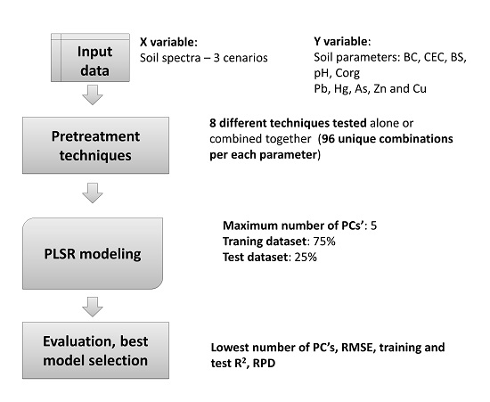
To fill these gaps in soil spectroscopic modelling, powerful statistical modelling, which can cope with many pre-treatment stages automatically to assess the best prediction models, was used and tested. This engine is termed PARACUDA^® and was designed to utilize parallel and automatic processing to build and process hundreds of diverse models in order to prevent errors or biases caused by an operator when taking the model setting decision. The following questions were asked when taking advantage of this innovative data mining approach:

• To what extent does the several preprocessing method improve the modelling?
• What is the contribution of the thermal infrared region (MWIR and in particular of the LWIR, as it is used in remote sensing applications) to the predictive capability of complex attributes that have no direct chromophores in the VIS–NIR–SWIR as well as MWIR and LWIR regions such as pH, base saturation and heavy metals?
• What is the influence of spectrometer parameters (e.g., different spectral resolution and region coverage) on the final model results?

2. Materials and Methods

2.1. Study Sites and Soil Samples

The study area was located in the Sokolov basin in the western part of the Czech Republic (Figure 1a), in a region affected by long-term extensive lignite mining. Due to the mining activities and coal burning power plants that were built in the immediate vicinity of the mined area, this region is one of the most contaminated areas of the Czech Republic where high levels of trace elements have been detected [31,32]. The soil was sampled from natural Norway spruce forest stands which surround the open-cast lignite mines in Sokolov, but have not been directly affected by the mining activities. However, the soil in all of the stands exhibits low pH [33].

Different bedrock characterizes the selected sites (

Table 1. Soil sample sites.

Site	Latitude (N)	Longitude (E)	Elevation (m.a.s.l.)	Distance from Open-Pit Mines (km)	Geological Unit
Erika	50°12′25″	12°36′17″	495	6.4	Staré Sedlo sandstones
Habartov	50°09′48″	12°33′28″	477	11.2	paragneiss, mica shist
Mezihorská	50°15′50″	12°38′17″	678	5.8	granites
Studenec	50°14′09″	12°33′00″	722	8.5	paragneiss, mica shist

). Metamorphic rocks, such as paragneisses, phyllites or mica-schist, underlie the sampling stands within the Habártov and Kovářská study site. In contrast, it is mainly intrusive rocks, such as granites, that underlie the sampling sites within the Mezihorská site and sedimentary rocks, such as sandstones, at the stands located in the Erika site. Both study sites have the same main soil type—Cryptopodzol/podzol.

Detailed field investigations preceded sample collection, In addition, trace element and heavy metal gradients were studied in situ using a portable Innov-x Alpha RFA spectrometer to ensure that the selected soil samples cover the whole gradient ranges found at the sites. At each forest stand (4 stands, Table 1), 10 soil samples were collected (40 samples in total). Tree litter was excluded and material was collected from the organo–mineral horizons (A + AB, depth of 10–30 cm). The soil material collected was air dried prior to sieving and then transported to the certified laboratories of the Czech Geological Survey. Exchangeable cations (Ca, Mg, K, Na) and Al were analysed in 0.1 M BaCl₂-extracts using atomic absorption spectrophotometry (AAS, Perkin-Elmer A Analyst 100). Soil pH was determined in distilled water and in 1 M CaCl₂ (ISO 103900). To measure Total Exchangeable Acidity (TEA), BaCl₂-extracts were titrated using 0.025 M NaOH to pH = 7.8. To measure the organic carbon (Corg) and selected trace elements (Cu, Zn, As, Hg) the samples were sieved <2 mm and homogenized, trace elements were then determined using flame atomic absorption spectrometry (FAAS) and, in the case of Hg, atomic absorption spectrometer (AMA254). Organic carbon (Corg) was determined by sulfochromic oxidation (ISO 14235). Cation exchange capacity (CEC) was calculated as the sum of exchangeable base cations (BC = Ca + Mg + K + Na) and TEA. Base saturation (BS) was determined as the fraction of CEC associated with BC.

Chemical analysis of the 40 samples within the dataset shows that the pH ranges were rather low—between 3.03 and 3.83. The other soil attributes showed high variations in the studied attributes (

Table 2. Descriptive statistics of the soil parameters studied.

	Min	Max	Mean	SD	Var	Skew
pH	3.03	3.83	3.45	0.16	0.03	−0.23
Corg (%)	2.08	9.71	5.29	2.23	5.02	0.36
BC (mmol(+)/kg)	1.69	111.35	26.16	26.83	720.22	1.41
CEC (mmol(+)/kg	61.07	183.50	109.88	32.74	1072.04	0.78
BS (%)	1.74	62.36	20.42	16.56	274.08	0.84
Hg (ppm)	0.06	0.26	0.15	0.07	0.01	0.26
As (ppm)	7.67	80.45	37.02	27.00	675.87	0.40
Cu (ppm)	5.50	26.40	13.93	7.24	52.36	0.41
Zn (ppm)	23.00	98.00	56.87	24.28	589.64	0.35
Pb (ppm)	30.00	147.00	77.40	37.52	1407.83	0.38

). Naturally, significant positive correlations (Pearson correlation coefficient r higher than 0.7) were found for Hg–C_ORG, Hg–Pb, As–Pb, Cu–Pb, Zn–Cu, BC–BS, Hg–CEC, Hg–BC, C_ORG–CEC, C_ORG–BC (Figure 2).

2.2. Spectral Measurements

Soil reflectance was measured at the laboratory using two different spectrometers: (i) a broad-band Full Spectral Range (FSR) reflectometer (designed by ABB Bomem, Québec City, QC, Canada) [34]—measured the reflectance of the soil samples across the optical and thermal regions (15,506–748 cm⁻¹; 0.64–13.36 µm) with a spectral resolution of 16 cm⁻¹; (ii) ASD FieldSpec3 spectroradiometer—measured the reflectance of the soil samples across the whole optical VIS–NIR–SWIR region (0.35–2.5 µm). The parameters of both spectrometers are shown in

Table 3. Technical specifications of the two spectrometers used.

Spectrometer Type	Spectral Range	Number of Bands	Spectral Sampling Interval
ASD	0.35–2.50 µm	2151	1.4 nm @ 350–1050 nm
			2 nm @ 1000–2500 nm
FSR	0.64–13.36 µm	1914	<1 nm @ 640–1100 nm
			From 1 to 5 nm @ 1050–2500 nm
			From 5 to 136 nm @ 2500–13,360 nm

. Both measurements were done using a high intensity contact probe. The ASD measurements were carried out according to [35]. A calibrated gold panel is built into the FSR instrument [36] and the FSR measurements were done under the following routine [34]: each soil sample was placed in a sampling cup, placed under the input port of the reflectometer and its reflectance spectrum was recorded. The reflectance spectra of the soil samples acquired from both spectrometers are shown in Figure 3.

2.3. Statistical Modelling Interface—PARACUDA

For this study a new computing engine that has been developed at RSL–TAU termed PARACUDA^® was used. This engine is an automated computing system developed to manage and deploy thousands of chemometric models and preprocessing combination methods in order to extract the best prediction model from a big data archive. It replaces the manual operation scheme usually deployed in chemometrics using other dedicated software such as the Unscrambler^® [37]. The system can be considered as data mining software for finding and utilizing hidden patterns and relationships within large and complicated databases with no human interaction. PARACUDA^® excels especially in handling large (spectral) data and modelling spectral measurements against chemical constitutes. This allows users to generate robust prediction models for soil properties (although it can work with other general databases).

One of the most advantageous characters of the abovementioned data mining system is the ‘all-possibilities’ approach (APA) scheme, where the system automatically applies linear and nonlinear modelling algorithms combined with several preprocessing methods to the data. The preprocessing algorithms include averaging, centring, smoothing, standardization, normalization and transformations among others. The modelling algorithms applied to the data are Artificial Neural Networks (ANN) and Partial Least Squares (PLS). Under the APA concept, the machine evaluates all preprocessing methods and their combinations and develops a unique model for every possible sequence resulting in up to 120 different combinations. This is an extremely computer power-consuming method and thus it runs on a grid based supercomputer with many processing cores for rapid analysis.

It must be stated that the APA approach was firstly tested by Zhao et al. (2015) [38] who proved the importance of considering multiple pathways for modelling spectral data. However, there are a few differences between the two approaches while the main one is the initial preprocessing or pretreatments procedure. Zhao et al. (2015) [38] tested five combinations of pretreatments: while this study analyzed a set of eight potential algorithms and evaluated each in different mutual combinations resulting in up to 120 valid combinations to be applied separately to the spectroscopic data.

The system is easy to operate via an excel plug-in and a web interface that enables fast and easy data transfers to the PARACUDA^® servers, changes to the modelling parameters for advanced users (a full automatic mode is the default) as well as controlling current jobs and monitoring their progress. The main PARACUDA^® excel plug-in screen enables dependent and independent datasets to be selected, the problem type to be selected (Function fitting or classification), notes to be entered for future reference and to finalize fine tuning of the PARACUDA operation including the data division process for validation, dimension reduction and modelling methodologies. Furthermore, preprocessing options and other advanced parameters are also available through the excel plugin.

For reliable results that represent the entire dataset as best as possible, the Conditioned Latin Hypercube Sampling (cLHS) method is used in the system [37]. The cLHS is a stratified random procedure that provides an efficient way of sampling variables from their multivariate distributions. Up to 1,000,000 semi-random (quantile) divisions are created and the distributions of the modelled values are examined. The variability of values within each sub-group is evaluated for each grouping iteration. The grouping with the most variability within each group is chosen as the best representation of the dataset and continues to the following steps. For this process it is important to make sure there is similarity in the values range and distribution in the calibration and validation groups.

PARACUDA^® pre-processes spectral datasets prior to analysis in order to remove any irrelevant information which cannot be handled properly by the modelling techniques. The system uses some of the most common preprocessing techniques: Savitsky–Golay Initial Smoothing [39]; Multiplicative Scatter Correction (MSC); Standard Normal Variate (SNV); Pseudo Absorptance (log(1/R) [40]; Continuum Removal [41]; First Derivative [42]; Second Derivative [43]; and Final Smoothing. The system applies possible combinations of the calculations in a specific order, optionally creating 120 new datasets. Each new dataset is the outcome of the preprocessing sequence applied to the data repetitively. For example, an optional sequence can be: Smoothing, Continuum Removal, First Derivative, and again Smoothing. All mathematically valid combinations applied to the original data result in a new archive of data-sets which are ready to be evaluated and modelled.

The system enables the user to adjust the training/test grouping ratio for the population. In this case the system was set to use 75% of the samples for training and 25% of the samples for testing. As previously mentioned, the data was divided into these groups based on the cLHS algorithm that ensured appropriate representation of the datasets. The results of all of the PLS models were then consolidated to statistically quantify the effects of the preprocessing method, as well as the training/test group selection process on the modelling results.

PARACUDA Model Setting

Due to the limited number of samples, PARACUDA was only used for the PLSR modelling. The PLSR models were built for diverse soil properties (BC, CEC, BS, pH, Corg, Pb, Hg, As, Zn and Cu) using three different spectral scenarios (see Figure 3):

• using the soil spectra acquired by the FSR spectrometer, which covers the whole optical and thermal range (0.6–13.3 µm, Scenario 1: Sc1)
• using the soil spectra acquired by the FSR spectrometer selecting the optical range only (0.6–2.5 µm, Scenario 2: Sc2)
• using the soil spectra acquired by the ASD spectrometer: the whole optical range (0.4–2.5 µm, Scenario 3: Sc3)

The 40 samples from the original dataset were automatically divided into a training dataset consisting of 30 samples, and a test set of 10 samples by the software, as described earlier. In order to avoid over fitting, an internal validation method (full cross-validation) was first run on the entire 40 samples to estimate the optimal number of Latent Variables (LV) on the PLSR models.

As previously discussed in this study, eight different preprocessing techniques and their combinations were tested under the PLSR modelling: Smoothing (SM), multiplicative Scattering Correction (MSC), Signal Normal Variate (SNV), Absorbance (ABS), Continuum Removal (CR), 1st and 2nd Derivative (FD and SD, respectively) and final smoothing (FSM). PLSR modelling was employed combining all logical combinations among the eight preprocessing techniques, while PLSR models were set to run identically (Figure 4) and employed on the three different scenarios described above (utilizing different spectral settings Figure 3).

After processing, the selection of the best models out of all the options were evaluated based on the following parameters: lowest number of factors as a measure of model robustness, the lowest root mean square error of prediction (RMSEP) as a measure of expected error in future predictions, the coefficient of determination (R²) and the Relative Percentage Difference (RPD).

As a result, for each of the parameters, 96 models were run for each spectral set (each spectral scenario), thus 288 PLSR models (3 × 96) were processed in all for each soil parameter (

Table 4. Statistics on the spectral preprocessing techniques of the best models found for the selected soil attributes while using PLSR modelling (SM: smoothing, FSM: final smoothing, MSC: Multiplicative Scatter Correction, SNV: Signal Normal Variate, ABS: absorbance, CR: continuum removal, FD: first derivative, SD: second derivative, (n): number of models found fulfilling the selection criteria: employed maximum of up to five PC’s, reached RPD higher than 1.5 and achieved the highest R²test, * model RPD was <1.5).

		Spectral Preprocessing
Soil Attributes	Scenario	SM	FSM	MSC	SNV	ABS	CR	FD	SD	(n)
BC	Sc1					x	x	x		3
		x							x
		x	x					x
	Sc2							x		1
	Sc3	x				x	x		x	2
		x					x		x
CEC	Sc1	x	x					x		1 *
	Sc2					x				1 *
	Sc3					x			x	1 *
BS	Sc1	x	x							1
	Sc2	x				x				1
	Sc3							x		1
pH	Sc1		x	x			x			1
	Sc2	x							x	1
	Sc3	x							x	1
Corg	Sc1		x			x				2
								x
	Sc2		x			x	x			1
	Sc3			x		x				1
Pb	Sc1	x	x						x	3
			x					x
			x					x
	Sc2	x				x	x			1
	Sc3		x					x		1
Hg	Sc1	x							x	1
	Sc2					x	x			1
	Sc3		x			x		x		1
As	Sc1		x				x			1
	Sc2					x	x			1
	Sc3		x			x		x		1
Zn	Sc1		x				x	x		1
	Sc2	x								1
	Sc3	x	x					x		1
Cu	Sc1		x							1
	Sc2		x							1
	Sc3	x	x	x			x			2

,

Table 5. PLSR Models for BC, CEC, BS, pH, C_org: the best model statistics using the three different spectral data sets as inputs: Scenario 1: Sc1 (0.6–13.3 µm, FSR spectrometer), Scenario 2: Sc2 (0.6–2.5 µm, FSR spectrometer), Scenario 3: Sc3 (0.4–2.5 µm, ASD spectrometer), * model where RPD was <1.5.

Soil Attribute (Spectrometer)	PC (n)	Test R2	RMSEP	SEP	SD	RPD
BC: Sc1	1	0.79	14.86	10.60	22.94	2.69
	2	0.86	12.91	9.01	23.09	3.16
	3	0.73	13.59	12.59	24.09	2.24
BC: Sc2	1	0.62	17.83	17.91	23.09	1.59
BC: Sc3	2	0.81	18.35	12.78	23.19	2.23
CEC: Sc1	3	0.62	21.46	22.89	36.96	1.42 *
CEC: Sc2	5	0.62	31.24	21.57	34.59	1.48 *
CEC: Sc3	2	0.49	23.69	25.23	34.57	1.32 *
BS: Sc1	5	0.83	11.56	7.76	17.71	2.13
BS: Sc2	5	0.71	10.57	10.17	17.84	1.62
BS: Sc3	1	0.81	8.87	7.61	14.60	2.26
pH: Sc1	3	0.44	0.07	0.08	0.10	2.25
pH: Sc2	1	0.68	0.07	0.06	0.10	3.05
pH: Sc3	1	0.77	0.05	0.04	0.09	4.23
Corg: Sc1	2	0.87	0.84	0.79	2.18	2.77
	1	0.81	1.01	1.02	2.18	2.16
Corg: Sc2	4	0.82	1.11	0.97	2.27	2.35
Corg: Sc3	3	0.85	1.00	0.97	2.18	2.26

and

Table 6. PLSR Models for heavy metals (Pb, Hg, As, Zn, Cu): the best model statistics using three different spectral data sets as inputs: Scenario 1: Sc1 (0.6–13.3 µm, FSR spectrometer), Scenario 2: Sc2 (0.6–2.5 µm, FSR spectrometer), Scenario 3: Sc3 (0.4–2.5 µm, ASD spectrometer).

Soil Attribute: Scenario	PC (n)	Test R2	RMSEP	SEP	SD	RPD
Pb: Sc1	2	0.89	12.64	12.96	37.93	2.94
	4	0.82	16.31	14.49	33.05	2.70
	2	0.89	14.06	13.69	39.29	2.69
Pb: Sc2	4	0.85	15.36	16.39	38.74	2.32
Pb: Sc3	4	0.65	15.85	15.07	23.13	2.61
Hg: Sc1	2	0.91	0.03	0.02	0.07	2.72
Hg: Sc2	5	0.72	0.04	0.04	0.07	1.68
Hg: Sc3	2	0.78	0.03	0.03	0.07	2.02
As: Sc1	5	0.81	11.74	12.25	28.30	2.13
As: Sc2	5	0.72	16.50	15.21	26.65	1.73
As: Sc3	5	0.85	11.74	12.55	28.32	2.08
Zn: Sc1	1	0.77	12.16	12.21	23.58	2.04
Zn: Sc2	3	0.84	11.83	11.93	24.26	2.08
Zn: Sc3	3	0.85	11.37	10.13	25.94	2.37
Cu: Sc1	5	0.99	2.09	1.40	7.01	5.27
Cu: Sc2	5	0.91	3.39	2.67	7.64	2.72
Cu: Sc3	5	0.93	3.03	3.13	6.72	2.37
	5	0.83	4.37	3.13	7.40	2.33

). Therefore, for 10 different soil attributes 2880 models were generated and evaluated. It should be emphasized that this arduous work was run automatically and took 60 min. An expert/operator consideration was only entered after the best model was selected in order to explain the spectral assignment of the model as will be discussed later.

3. Results

3.1. PLSR Prediction Model Assessment

Table 4, Table 5 and Table 6 present the results of the best analytical runs. To select the number of the most significant components the eigenvalue plots were generated for all the soil variables studied. It was found that the first five PC’s explained most of the data variance. Therefore, the PLSR models selected employed a maximum of up to five PC’s, reached a RPD higher than 1.5 and achieved the highest R² for the test data set (R²test). In some cases it was not possible to find any model that showed RPD higher than 1.5 and these models were marked with * in Table 4, Table 5 and Table 6.

Table 4 shows the best prediction models found, respectively the preprocessing techniques employed on spectral data prior to modelling, either alone or in all possible mutual combinations. Summarizing these results it can be said that preprocessing spectral data prior to modelling is an important step. For all of the parameters, the models achieving the best results employed some kind of preprocessing techniques (usually a combination of two or three of them). In other words, no model without preprocessing achieved better results than those employing the preprocessing techniques. For most of the models which were run, the smoothing (smoothing and/or final smoothing) was found to be beneficial, especially in combination with derivative transformation (1st or 2nd derivatives). If the optical spectral data are used as an input (Sc2 and Sc3), the transformation to absorbance was also a preferable preprocessing step that resulted in increasing the model’s quality.

Table 5 and Table 6 show the best models with statistics as follow: number of PC’s, R²test, Root Mean Square Errors (RMSE), Standard Deviations (SD) and Regression Point Displacements (RPD’s). Based on the guidelines given by [44], the prediction models obtained were categorized into five groups which are then summarized in

Table 7. The prediction models obtained were categorized into five groups (1 is the best and 5 the worst score) based on the guidelines given by [44], further described in Section 3.1). If the same score is obtained, the model with the higher R²test is marked with *. Scenario 1: Sc1 (0.6–13.3 µm, FSR spectrometer), Scenario 2: Sc2 (0.6–2.5 µm, FSR spectrometer), Scenario 3: Sc3 (0.4–2.5 µm, ASD spectrometer).

Soil Attributes	Sc1	Sc2	Sc3
BC	2	4	3
CEC	5	5	5
BS	2	4	3
pH	5	3	3 *
Corg	2 *	2	2
Pb	2 *	2	4
Hg	2	4	3
As	3	4	3 *
Zn	3	3	3 *
Cu	1	3	3

: score 1 (excellent prediction): RPD and R²test higher than 3.0 and 0.9 respectively, score 2 (good predication): RPD values from 2.5–3.0 and R²test between 0.82–0.90, score 3 (approximate prediction): RPD values from 2.0–2.5 and R²test between 0.66–0.81, score 4 (possibility to distinguish between high and low values): RPD values from 1.5–2.0 and R²test between 0.50–0.65, score 5 (unsuccessful prediction): RPD values lower than 1.5 or R²test lower than 0.5.

To summarize, when using PARACUDA^® the best predictability was obtained for Cu (R²test > 0.9, RPD > 3) followed by Pb, Corg and Hg (v R²test > 0.82, RPD between 2.5 and 3.0) and by BC, BS, Zn and As (validation data set R² > 0.8, RPD between 2.0 and 2.5).

For some variables it was possible to find more than one model having high RPD’s (Table 5 and Table 6):

• when the FSR scenario (Sc1) was employed: BC and Pb (three models), Corg (two models)
• when the ASD scenario (Sc3) was employed: Cu (two models)

On the other hand, CEC was found to be difficult to predict even when using the PARACUDA^® and being able to assess 288 different models (in Table 4 marked with *).

The information from the thermal region (Sc1) brought significant benefits to the modelling of base cations (BS), base saturation (BS) and organic C (C_org) content as well as for some heavy metals such as: Pb, Hg, Cu and As (Table 6 and Table 7). On the other hand, the high spectral resolution across the optical VIS–NIR–SWIR range provided by the ASD spectrometer (Sc3) was more beneficial for modelling pH and Zn (Table 6 and Table 7).

3.2. Spectral Sensitivity Assessment

As described in Section 3.1, the statistics revealed the following results:

• High spectral resolution covering the whole optical range (the spectral information acquired by the ASD spectrometer), was found to be more beneficial for modelling pH, Zn, As and C_org (Sc 3)
• The information in the thermal region (MWIR and LWIR) improved the predictive capabilities for BC, BS and C_org content as well as for such heavy metals as Pb, Hg and Cu (Sc1).

The intention was to further test if the above described trends (the cases when a high-spectral-resolution optical range gives better predictions vs. the cases when a lower spectral resolution covering optical and thermal ranges gives better predictions than the latter one) can be explained in terms of spectral assignments. Spectral assignment is very important information in chemometrics [45], especially when a small data set is analysed. If spectral assignment cannot be found, all models might remain questionable, as no physical chemical basis is encountered. The version of the Paracuda used at the time of processing did not provide an interface to visualize spectral implications and assignments (later versions will include this function). Accordingly, to be able to explain which particular wavelengths are the most important for predictions and to visualize the spectral implications of the studied soil attributes the Pearson’s correlation coefficients (r) were calculated between the attributes and the measured reflectance values (Figure 5, Figure 6 and Figure 7) using the statistical software (SW) SPSS.

3.2.1. Demonstrating the Benefit of Scenario 3 When the Whole Optical Region (0.4–2.5 µm) Is Covered at a High Spectral Resolution

As already discussed, the high spectral resolution within the wider VIS–NIR–SWIR optical range (the spectral information obtained by the ASD spectrometer), was more beneficial for modelling pH, Zn and As. For those attributes the Person’s correlation coefficients (r) calculated over the optical ranges of both spectrometers, ASD and FSR, are displayed in Figure 5. In addition to the above attributes, the C_org is also displayed to demonstrate the spectral assignments of the organic component. To be able to discuss and compare these results with those previously published,

Table 8. Band assignments of identified VIS–NIR–SWIR wavelengths (these were compiled from [45,46]).

Wavelengths (µm)	Possible Assignment	Remark
0.400–1.200	Electronic transitions	Iron-bearing minerals
0.450, 0.520–0.533, 0.560–0.575, 0.630–0.640, 0.660–0.680		Organic C
1.400, 1.900	Water absorption
2.190–2.290	OH–stretching and bending combination vibrations	Phyllosilicates
2.270, 2.310, 2.350	C–H stretching	Organic matter

shows band assignments of identified VIS–NIR–SWIR wavelengths, which were compiled from [45,46].

The key wavelengths within the VIS–NIR–SWIR optical range for the C_org (Figure 5) were found to be between 0.40–0.54 µm (r lower than −0.77), 0.63–0.73 µm (r lower than −0.76–0.7), 2.26–2.32 µm and 2.35 µm (r lower than −0.67). These spectral assignments characterized organic matter or biomass [14,47].

The key wavelengths for pH were located in the VIS and NIR regions, the highest negative correlations (r between −0.4 and −0.3) were found for the spectral region between 0.40–0.53 µm and then between 0.82–1.00 µm (r between −0.3 and −0.27). These wavelengths are usually assigned to electronic transitions of Fe-oxides [14,48,49,50] which are highly correlated with pH. The inter-correlation of the chromophoric property (in this case Fe-oxides) to the non-chromophoric one (in this case pH) is discussed in [44]. They demonstrated significant model prediction of non-chromophoric attributes in soils by the inter-correlation mechanism. It is well known that the VIS–NIR region can be used to differentiate between diverse iron oxides which are stable under different pH ranges [28,51,52,53] and accordingly to serve as a spectral assignment indicator for pH. As demonstrated in Figure 5, the ASD spectrometer, characterized by a wider optical range while having a high spectral resolution, is more advantageous in this case than the FSR spectrometer, which is characterized by a shorter optical range in the VIS–NIR region. As a result the FSR is more limited in detecting and discriminating diverse Fe-oxides and thus not optimal for predicting pH. Similarly, the important wavelengths of Zn are assigned to the same VIS–NIR regions as pH, 0.40–0.53 µm (r between −0.54 and −0.44) and 0.84–1.00 µm (r between −0.435 and −0.453) again indicating the inter-correlation mechanism by the Fe-oxides assignments. In addition, wavelengths between 2.35 and 2.366 µm show higher negative correlations (below −0.4). This spectral region can be assigned to C biomass [14,54] showing that Zn can also be associated with C biomass in the soil samples under study (again via the chromophoric property). Also in this case, the better spectral coverage of the ASD spectrometer (e.g., spectral range) allowed better determination of both iron oxides and C biomass. The As follows a similar pattern as described for Zn, except that the assignments between 0.63 and 0.73 µm characterizing C_org are better pronounced. With the examples of Zn and As, the advantage of the better spectral coverage of the ASD spectrometer, allowing better differentiation between iron oxides and the organic component, is also demonstrated.

When comparing the sensitivity results obtained by the ASD and FSR spectrometers for the same attributes, a common general trend was found (lowest negative correlations found for C_org followed by Zn, As and pH). However, for the spectrum obtained by the FSR spectrometer, lower correlations were found (Figure 5b) (between −0.45 and −0.5) as compared to the ASD spectrum (between −0.2 and −0.8) (Figure 5a). These results demonstrate that the spectral optical coverage of the FSR spectrometer (0.6–2.5 µm) does not allow such detailed differentiation among iron minerals and organic matter as is possible with the ASD spectrometer (0.4–2.5 µm).

3.2.2. Demonstrating the Benefit of Scenario 1 When Optical and Thermal Regions (0.6–13.3 µm) Are Combined

Combining the optical and thermal region together in Scenario 1 brought significant benefits to the modelling of base cations (BC), base saturation (BS) and organic C (C_org) as well as to heavy metals such as Pb, Hg and Cu. For these soil attributes the Person’s correlation coefficients (r) calculated over the VIS–NIR–SWIR and MWIR–LWIR regions are displayed in Figure 6 and Figure 7, respectively.

Similarly as in the case of As, Zn and pH, the important wavelengths in the VIS–NIR (Figure 6) indicate inter-correlation with Fe-oxides, in addition, the absorptions in the SWIR region at 2.21 µm and 2.34 µm indicate inter-correlations with clay minerals and C biomass, respectively. The most important ranges in the MWIR–LWIR region were identified as follows: 2.77–3.83 µm (3600–2580 cm⁻¹), 5.75–6.40 µm (1740–1560 cm⁻¹), 8.15–9.52 µm (1226–1050 cm⁻¹) and 10.90–12.20 µm (920–825 cm⁻¹) (Figure 7). The positive correlation peaks, which are highest around 5.2 µm (1900 cm⁻¹) and 7.7 µm (1300 cm⁻¹), characterize the absorption shoulder positions and demonstrate that the higher the shoulder is, the higher the contents of the studied soil attributes are. On the other hand, absorption wavelengths that correlate with the soil attribute contents are characterized by negative correlations, the stronger the relationship between the soil attribute and the absorption depth, the more significant the negative correlation and thus a lower r is obtained. In

Table 9. Key wavelength ranges within MWIR–LWIR identified in this study employing a sensitivity analysis. As the results published by the scientific community commonly use the wavelength (µm) and/or wavenumber (cm⁻¹) scales, both scales are used to make the results comparable and universal.

Soil Parameter	MWIR–LWIR
	µm	cm−1
pH	2.76; 8.42; 11.79	3619; 1188; 848
CORG	2.77–3.87 (absorption: 2.80);	3600–2580 (absorption: 3564);
	5.75–6.62 (absorptions: 6.00 and 6.33);	1740–1510 (absorptions: 1666 and 1580);
	8.16–9.52 (absorptions: 8.70, 9.26);	1226–1050 (absorptions: 1150; 1080);
	10.75–12.12 (absorption: 11.79)	930–825 (absorption: 848)
BS	2.76; 8.42; 11.79	3619; 1188; 848
BC	2.76; 8.42; 11.79	3619; 1188; 848
CEC	2.77–3.87 (absorption: 2.80);	3600–2580 (absorption: 3564);
	8.16–9.52 (absorptions: 8.70, 9.26);	1226–1050 (absorptions: 1150; 1080);
	10.75–12.12 (absorption: 11.79)	930–825 (absorption: 848)
Pb	2.77–3.87 (absorption: 2.80);	3650–2780 (absorption: 3602);
	5.75–6.62 (absorptions: 6.00 and 6.33);	1750–1550 (absorptions: 1666);
	8.16–9.52 (absorptions: 8.70, 9.26);	1226–1050 (absorptions: 1150; 1080);
	10.75–12.12 (absorption: 11.79)	930–825 (absorption: 848)
Hg	2.77–3.87 (absorption: 2.80);	3650–2780 (absorption: 3556);
	5.75–6.62 (absorptions: 6.00 and 6.33);	1750–1550 (absorptions: 1666; 1573);
	8.16–9.52 (absorptions: 8.70, 9.26);	1226–1050 (absorptions: 1150; 1080);
	10.75–12.12 (absorption: 11.79)	930–825 (absorption: 848)
As	2.77–3.87 (absorption: 2.80);	3650–2780 (absorption: 3602);
	8.16–9.52 (absorptions: 8.70, 9.26);	1226–1050 (absorptions: 1150; 1080);
	10.75–12.12 (absorption: 11.79)	930–825 (absorption: 848)
Cu	2.77–3.87 (absorption: 2.80);	3650–2780 (absorption: 3602);
	5.75–6.62 (absorptions: 6.00 and 6.33);	1750–1550 (absorptions: 1666);
	8.16–9.52 (absorptions: 8.70, 9.26);	1226–1050 (absorptions: 1150; 1080);
	10.75–12.12 (absorption: 11.79)	930–825 (absorption: 848)
Zn	2.77–3.87 (absorption: 2.80);	3650–2780 (absorption: 3602);
	8.16–9.52 (absorptions: 8.70, 9.26);	1226–1050 (absorptions: 1150; 1080);
	10.75–12.12 (absorption: 11.79)	930–825 (absorption: 848)

the key wavelength ranges identified within the MWIR–LWIR regions when using the sensitivity analyses are assigned. To compare the results,

Table 10. Band assignments of identified MWIR–LWIR wavenumbers (these were compiled from [46,53,54,55,56,57,58]. As the results published by the scientific community commonly use the wavelength (µm) and/or wavenumber (cm⁻¹) scales, both scales are used to make the results comparable and universal.

Wavelengths (µm/cm−1)	Constituent/Structural Assignment	Remark
2.778–3.333 µm/3600–3000 cm−1	O–H stretching bands, H2O bending near 3.1 µm	Overtones and combinations of phyllosilicates
		2.66, 2.73 µm are fundamental modes in H2O molecule
2.762–2.994 µm/3620–3340 cm−1	H2O–stretching bands	Overtones and combinations of phyllosilicates
3.410–3.571 µm/2932–2800 cm−1	C–H bands of organic compounds	Overlap with inorganic components such as clays and silica
5.747–5.889 µm/1740–1698 cm−1	C=O groups in carboxylic acids, aldehydes and ketones	C–O groups in soil organic matter
6.087–6.250 µm/1640–1600 cm−1	Amid I band (C=O, C–N) of proteins, C=O of carboxylic acids and ketones	C–O groups in soil organic matter
7.812–8.333 µm/1280–1200 cm−1	C=O and O–H of COOH	soil organic matter
8.547–10.526 µm/1170–950 cm−1	C–O–C stretching of polysaccharides	soil organic matter
8.1–9.5 µm	Si–O bond stretching vibrations	quartz
8.771–12.048 µm/1140–830 cm−1	Tetraeder SiO4 stretching and banding vibrations	silicates
10.929–12.658 µm/915–790 cm−1	OH banding vibrations	phyllosilicates

shows band assignments of identified wavenumbers compiled from [46,53,54,55,56,57,58].

The key wavelengths for BS as well as BC were found for a region between 2.76 and 3.20 µm (3625–3120 cm⁻¹) (for both r lower than −0.4) and then 11.8–12.0 µm (843–833 cm⁻¹) (r for BS lower than 0.4 and for BC lower than −0.35 respectively). Both these ranges are assigned to phyllosilicates (Table 10) showing that for these attributes it is beneficial if such a mineral phase can be spectrally detected.

C_org exhibits negative correlation lower than −0.5 across a wide range between 2.77 and 3.60 µm (3600–2778 cm⁻¹), that can be assigned to overtones and combinations of phyllosilicates and organic compounds (Table 10). Then negative correlations lower than −0.4 are associated with the following ranges: 5.83–6.14 µm (1712–1627 cm⁻¹), 8.15–8.80 µm (1226–1134 cm⁻¹), 10.12–9.40 µm (1095–1064 cm⁻¹) and 11.07–12.00 µm (902–833 cm⁻¹). The range between 5.83–6.14 µm (1712–1627 cm⁻¹) is associated with C–O groups in soil organic matter, the range 8.15–8.80 µm (1226–1134 cm⁻¹) to COOH, the range 10.12–9.40 µm (1095–1064 cm⁻¹) can be possibly assigned to C–O–C stretching of polysaccharides as well to silica content (SiO₄) and the 11.07–12.00 µm (902–833 cm⁻¹) to phyllosilicate content.

When analysing the correlation across the MWIR–LWIR wavelengths for Cu and Pb, a wide range between 2.77–3.40 µm (3600–2923 cm⁻¹) exhibits correlations lower than −0.6 (possibly assigned to phyllosilicates). Apart from this, the range between 8.26 and 9.30 µm (1210–1070 cm⁻¹) shows negative correlations lower than 0.6 for Cu and lower than 0.55 for Pb. This demonstrates that Cu and Pb are associated with phyllosilicates and quartz as well as with the organic phases in the studied soils.

4. Discussion

The PARACUDA^® engine, due to its automatic processing, allowed a systematic assessment of what effects preprocessing techniques have on prediction model validity. Some preprocessing strategies have been tested before; Gholizadeh et al., 2015 [10] achieved the best results to predict potentially toxic elements (As, Cd, Cu) using Support Vector Machine Regression (SVMR) when employing Sawitzky–Golay smoothing together with derivative analysis as a pretreatment technique. 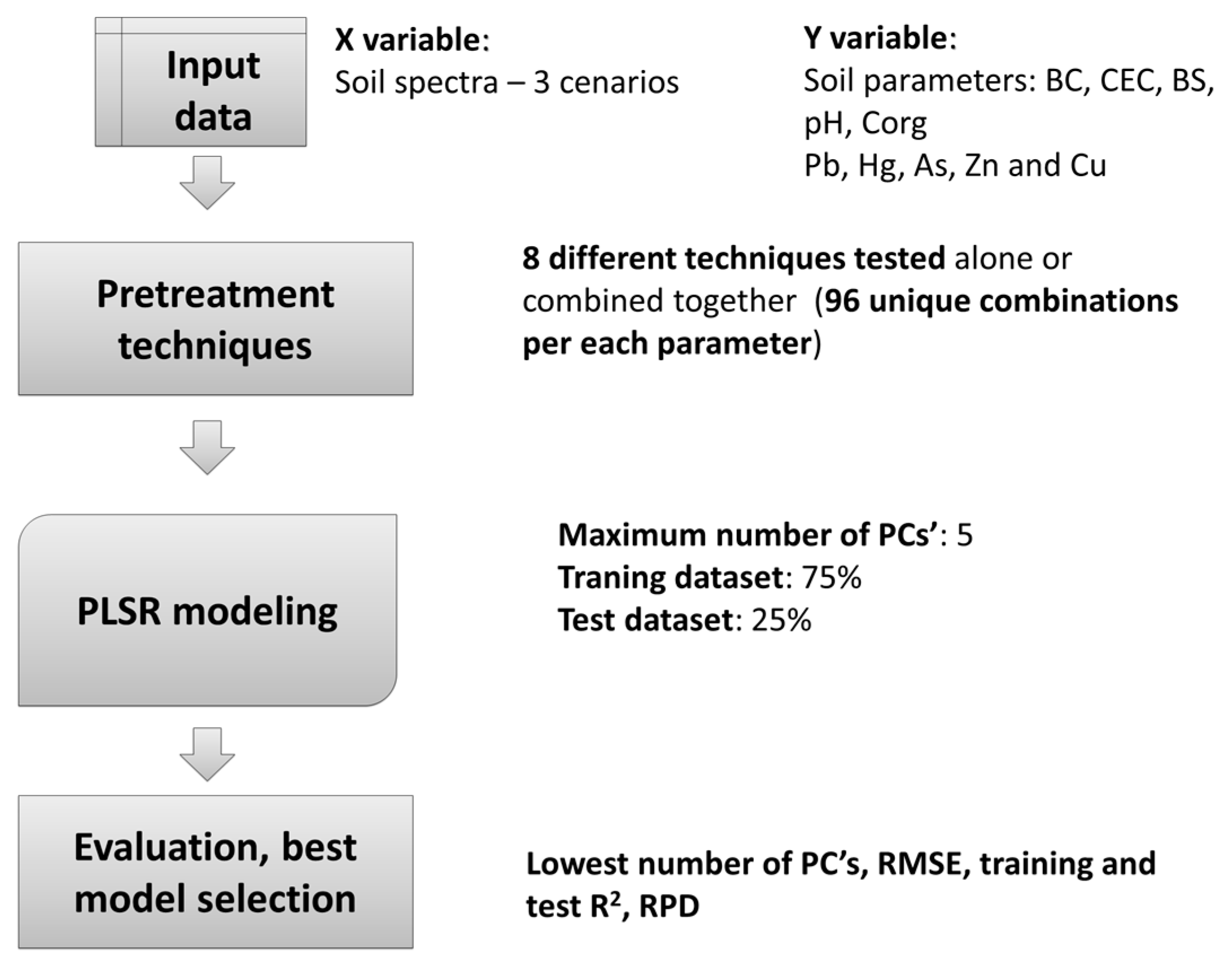Nocita et al., 2014 [59] tested several preprocessing techniques (CR, SNV, Sawitzky–Golay smoothing filter and the 1st and 2nd derivative) prior to employing PLSR modelling of soil organic content (SOC) when using the Lucas dataset and concluded that the Sawitzky–Golay smoothing and 1st derivative improved model prediction validity while the 1st derivative analyses improved the model’s performance for organic soil the most. In this study, the evaluation of 2880 models confirmed that the preprocessing of spectral data prior to modelling is an important step. For all of the soil attributes, the models achieved the best results when some kind of preprocessing techniques were employed (usually a combination of two or three of them). For most of the models run, smoothing (smoothing and/or final smoothing) was beneficial, especially in combination with derivative transformation (1st or 2nd derivatives).

PARACUDA^® was used to find the best estimation models of diverse soil attributes reaching the highest validity. A similar systematic approach was tested by Zhao et al., 2015 when using a processing trajectory to optimize non-systematic parameters (e.g., spectral pretreatment, latent factors and variable selection) and demonstrating better efficiency of using this approach to model the relative content of water in corn. It can be concluded that the data mining engine presented here can serve as an efficient tool to find the best prediction models. Apart from CEC, it was possible to find satisfactory predictions for the other modelled attributes (Cu considered as excellent prediction: RPD and R²test higher than 3.0 and 0.9 respectively; C_org, BC, BS, Pb, Hg models denoted as good prediction: RPD values from 2.5–3.0 and R²test between 0.82 and 0.90). Approximate quantitative predictions were achieved for As, Zn and pH (RPD values from 2.0 to 2.5 and R²test between 0.66 and 0.81). The values of CEC generally characterizing the studied Norway spruce forest soil dataset were high (mean: 109.8 mmol(+)/kg, standard deviation: 32.7 mmol(+)/kg) when compared to the studies published by [60,61]. This can be the reason why the CEC prediction was worse (RPD = 1.48, R²test = 0.62). For heavy metals, the results are comparable or even better than those published by [10] when employing SVM modelling together with the 1st derivative as a pretreatment technique or by Bray et al. (2009) [62] who used an ordinal logistic regression technique to predict Zn, Cu, Pb and Cd.

However, it needs to be noted that the results published by different groups or researchers are not consistent in the manner of defining the accuracy that can be achieved in predicting different heavy metals or other attributes which do not show any direct spectral chromophores. As they do not show any direct spectral chromophores, the mechanism of detecting them using infrared spectroscopy is thus attributed to their relationship with other soil components that have direct spectral chromophores. Therefore, for different case studies, such attributes can be predicted at different accuracy levels. For instance, heavy metals can be modelled due their associations with soil components such as: organic matter, clay minerals and Fe/Al oxides. These indirect relationships have previously been explored in pedotransfer functions (PTFs) [28]. For instance [63,64] demonstrated that various PTFs can be used to predict the adsorption of metals as a function of soil carbon content, CEC and pH. Furthermore, Choe et al. (2008) [65] proposed a binding mechanism based on the surface complex model where metals can bind to the hydroxylated mineral surface thus affecting the absorptions characteristic for Fe, Al, Mn oxides and clay minerals or organic matter. Therefore, in each case study, the results depend on the local geochemical conditions and thus the results are highly site-specific.

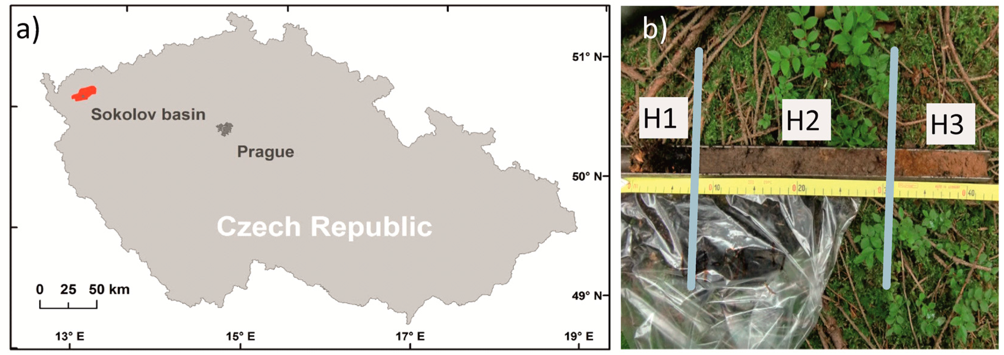
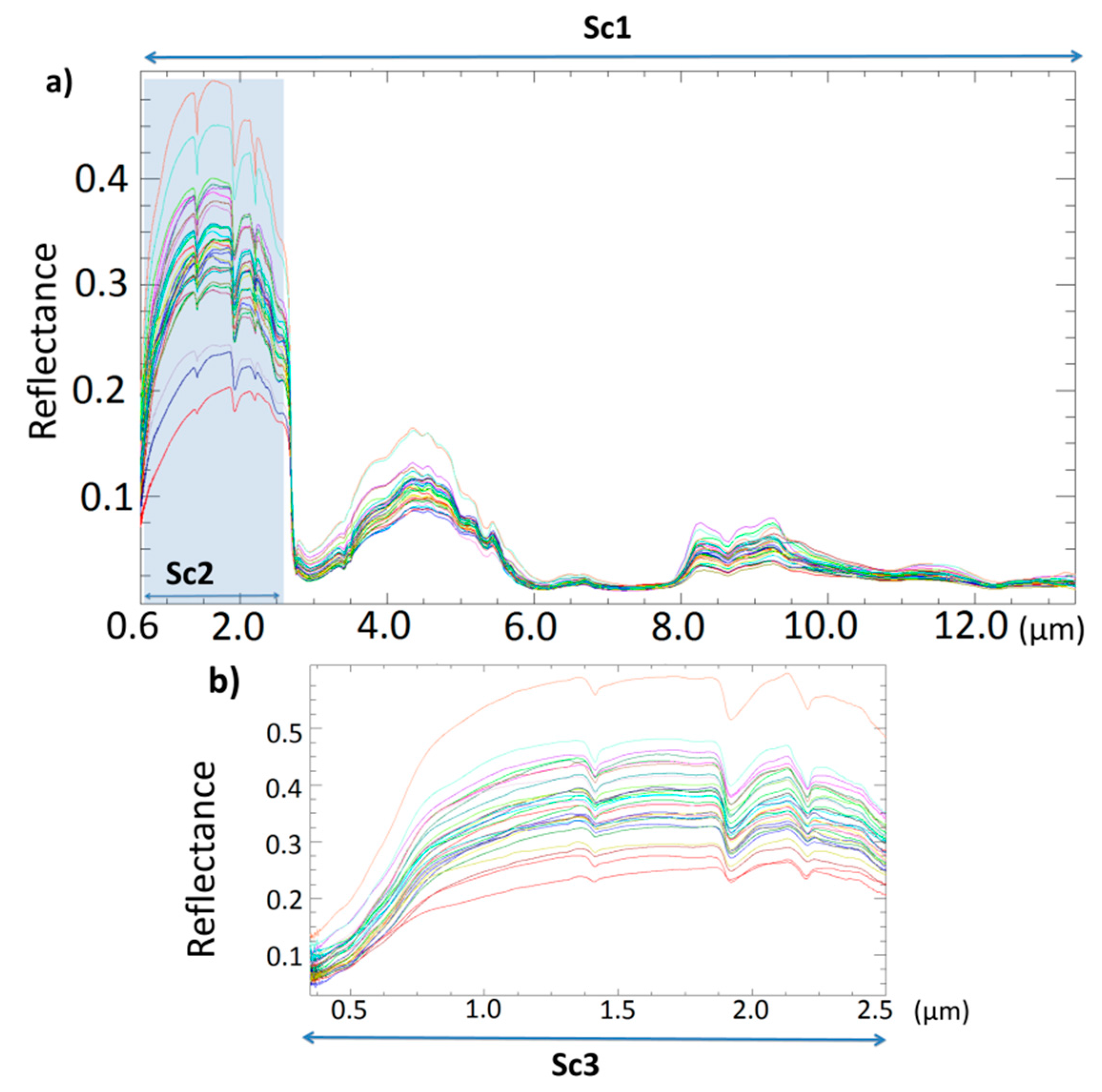
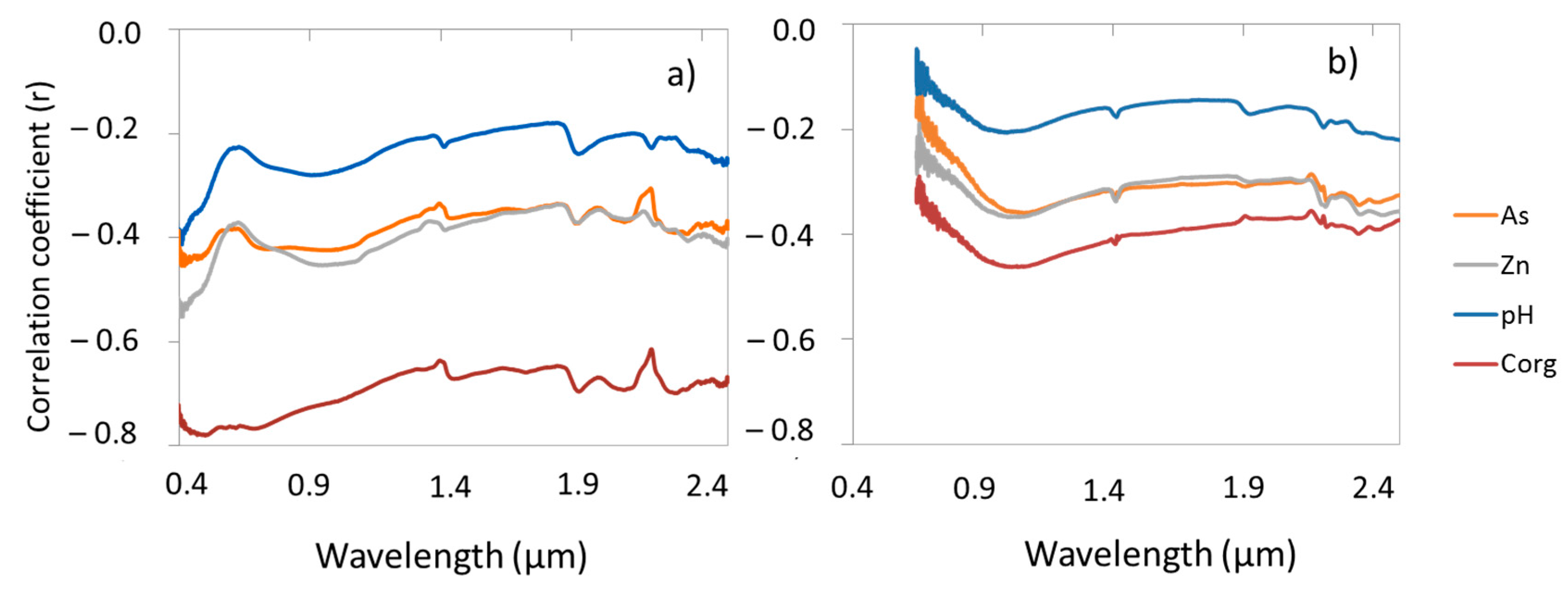
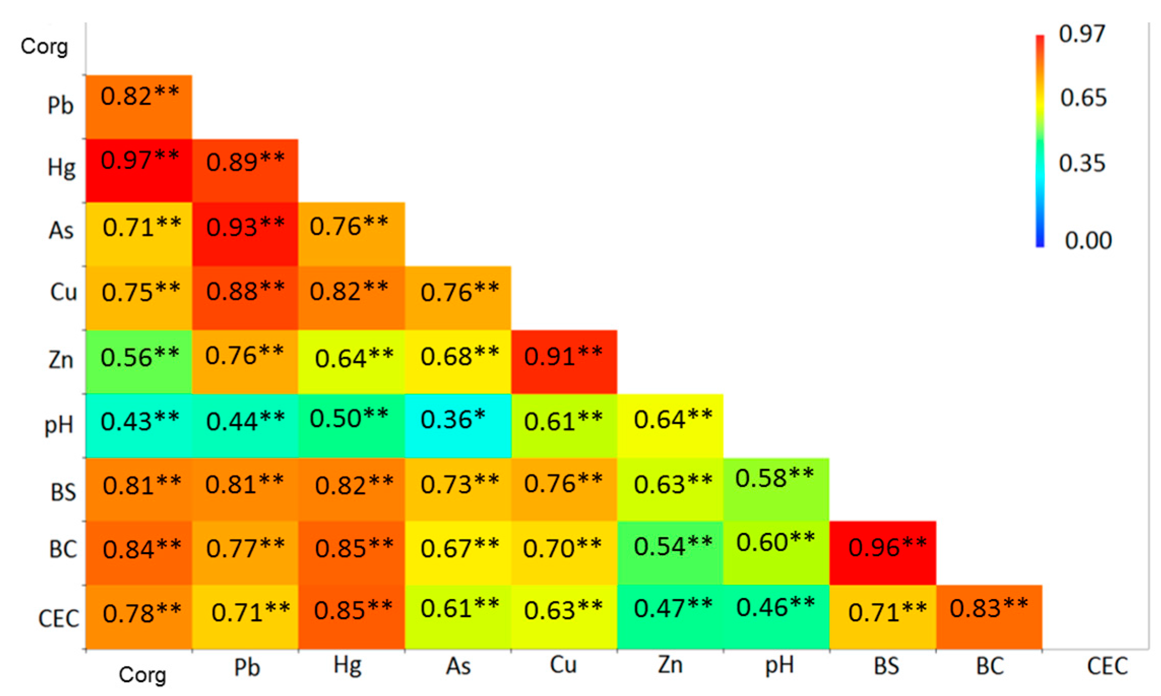
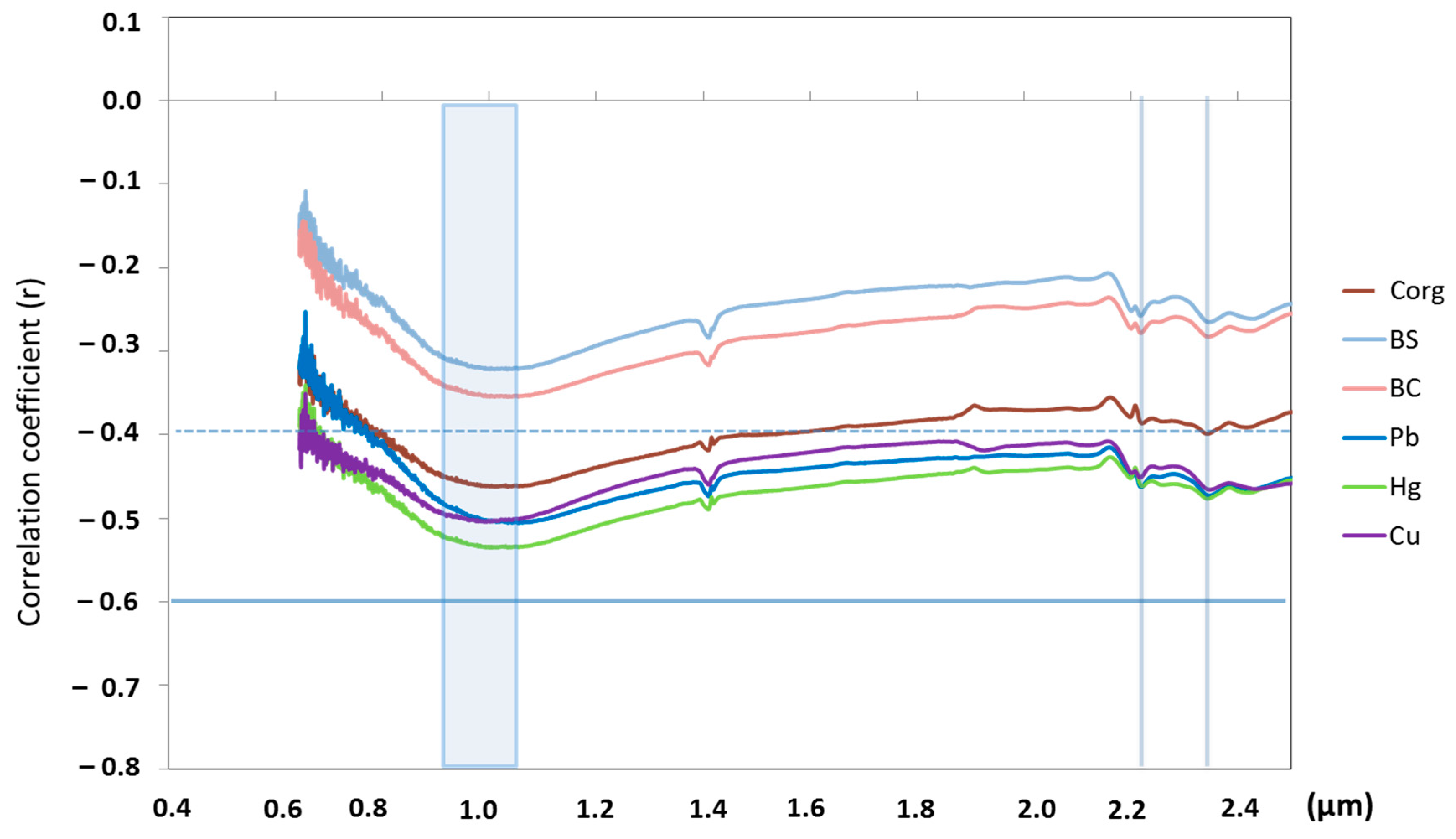
Due to the limited number of samples analysed (40 samples) and due to the fact that they were collected within one region, these results are also site-specific. However, it shows how the processing scheme presented here and the PARACUDA^® engine can be used to find the best prediction models as well as to get a better understanding of the geochemical properties of the samples studied. Employing statistical modelling with the aid of the system, allowed two groups or mineral associations to be defined: First group—Zn, As and pH—which can be predicted in a more accurate way using high spectral resolution spectra covering the whole optical range (ASD reflectance, 0.4–2.5 µm, Scenario 3)—and the second group—BC, BS, Pb, Hg, and Cu—for which more reliable predictions can be achieved when working with the spectrum covering shorter optical range and the thermal region (MWIR and LWIR, Scenario 1). 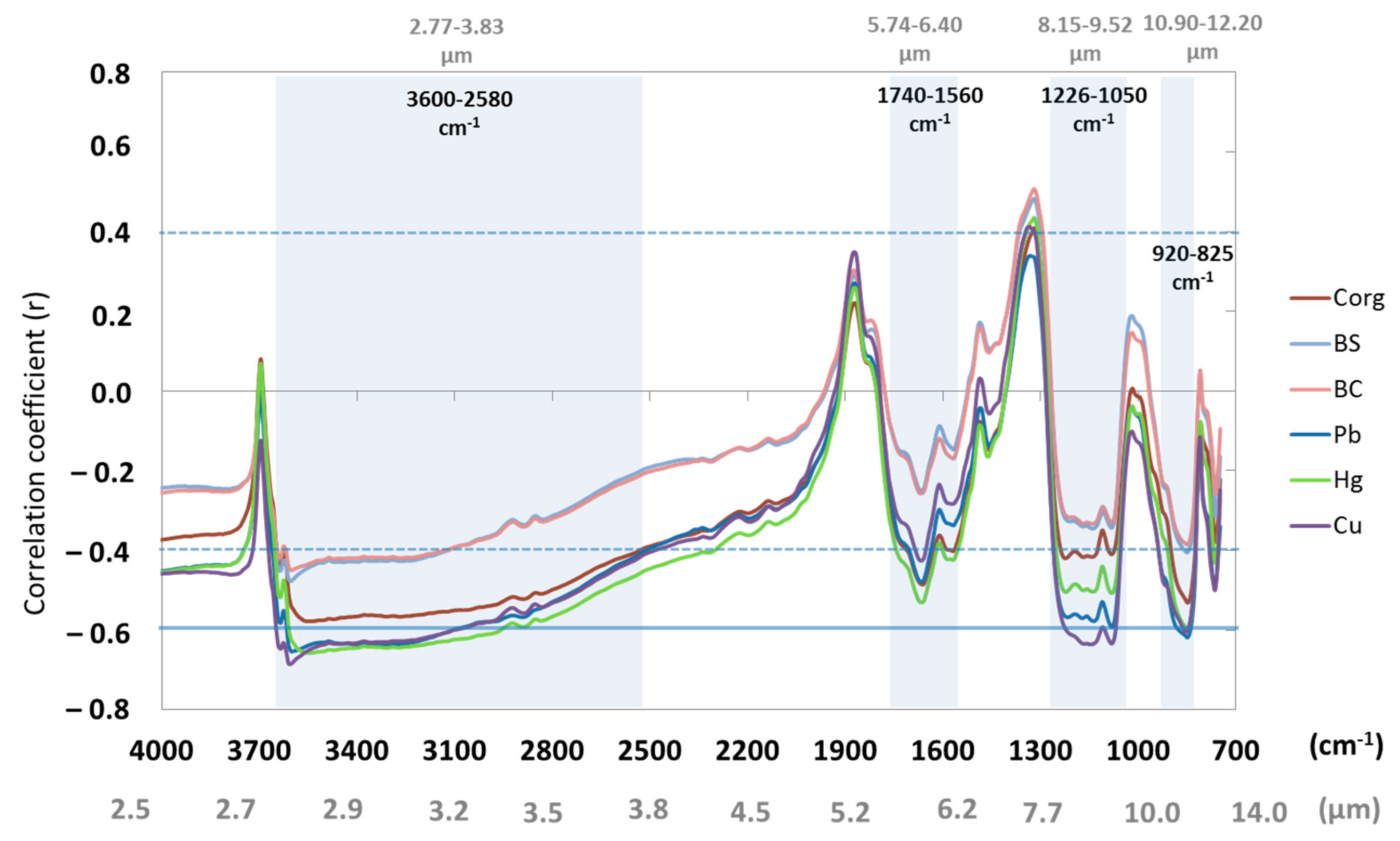Basically the same groups were defined when analysing the linear correlations among their chemical concentrations (Figure 2). It has been explained that pH, as well as Zn and As, show indirect spectral indications to iron oxides, organic matter and clay minerals (Figure 5). This relationship was also described in [33] where multivariate statistics were employed on a chemical analysis characterizing diverse horizons within the soil profile in order to define a conceptual model for the chemical and biochemical processes taking place in the studied soil–tree system. On the other hand, the second group (BC, BS, Pb, Hg, and Cu) has a stronger relationship to phyllosilicate content together with organic component (C_org). Logically, different TPHs can be used to predict these two groups (pH, Zn, As vs. BC, BS, Pb, Hg, and Cu). It has been demonstrated that the statistical analysis of spectral assignments can add important and reliable information about the non-chromophoric properties, just as laboratory methods provide. Furthermore, the indirect relationships to diagnostic soil constituent absorption features can be analysed to help to resolve the heavy metal’s abundances and geochemical form (e.g., speciation) despite the argument some scientists have raised [66]. This is key information for understanding the chemical behaviour of heavy metals in the environment studied.

Based on these results, it is possible to support the suggestion given by [61], that the use of portable VIS–NIR–SWIR together with MWIR–LWIR instruments has a potential to replace many conventional techniques of soil analysis. Whereas optical field spectrometers are becoming very popular and more and more frequently used, the price for a MWIR–LWIR portable instrument is still too high and remains unaffordable for most researchers. Nonetheless, as recently also demonstrated by others [12,67] these results strengthen the idea that future satellite systems should be designed to work in both the optical and thermal regions (e.g., HyspIRI) in order to better evaluate heavy metals on the Earth’s surface as well as to improve the modelling capability of attributes in complex soil systems. This is also relevant for field and laboratory work.

5. Conclusions

The APA data mining engine termed PARACUDA^® proved to be a powerful tool to assess the spectral performances of different spectrometers in order to achieve the best prediction models. This task cannot be achieved by the traditional and regular method that uses manual analyses and a subjective consideration by an expert/operator. For 10 soil attributes, the evaluation of 2880 models proved that preprocessing spectral data prior to modelling is an important step. For all of the attributes, the models achieving the best results employed some kind of preprocessing techniques (usually a combination of two or three of them). For most of the models run, smoothing (smoothing and/or final smoothing) was beneficial, especially in combination with derivative transformation (1st or 2nd derivatives).

Using the engine it was possible to find excellent (Cu) or good models (C_org, BC, BS, Pb, Hg) for most of the modelled attributes. Approximate quantitative predictions were achieved for As, Zn and pH. On the other hand, for the tested soils, the CEC was found to be difficult to predict even when using the PARACUDA^® and being able to assess 288 different models for this soil attribute. This can be explained by the rather high CEC values characterizing this forest soil dataset.

The information from the thermal region (MWIR and LWIR) brought significant benefits to modelling base cations (BS), base saturation (BS) and organic C (C_org) as well as such heavy metals as Pb, Hg, Cu and As. On the other hand, the wider optical-range coverage (ASD spectrometer) was more beneficial for modelling pH and Zn. These two attributes showed a high affinity to iron oxides, thus, in this case, the spectra acquired by the ASD spectrometer, which covers the optical range between 0.35–2.5 µm at a high spectral resolution, resulted in better predictions. The sensitivity analyses allowed identification of the wavelengths across the optical and thermal regions that were found to be important to predict selected soil attributes. Furthermore, it has been shown how the processing scheme presented here and PARACUDA^® can be used to obtain a better understanding of the geochemical properties of the samples studied (e.g., mineral associations). This is key information for understanding the chemical behaviour of heavy metals in the environment studied.

References

1. Soriano-Disla, J.M.; Janik, L.J.; Viscarra Rossel, R.A.; Macdonald, L.M.; McLaughlin, M.J. The performance of visible, near- and mid-infrared reflectance spectroscopy for prediction of soil physical, chemical, and biological properties. Appl. Spectrosc. Rev. 2014, 49, 139–186. [Google Scholar] [CrossRef]
2. Gobrecht, A.; Roger, J.M.; Bellon-Maurel, V. Major issues of diffuse reflectance NIR spectroscopy in the specific context of soil carbon content estimation: A review. Adv. Agron. 2014, 123, 145–175. [Google Scholar]
3. Sørensen, L.K.; Dalsgaard, S. Determination of clay and other soil properties by near infrared spectroscopy. Soil Sci. Soc. Am. J. 2005, 69, 159–167. [Google Scholar] [CrossRef]
4. Sánchez, J.C.; Barrón, V.; del Campillo, M.C.; Rossel, R.V. Reflectance spectroscopy: A tool for predicting soil properties related to the incidence of Fe chlorosis. Span. J. Agric. Res. 2012, 10, 1133–1142. [Google Scholar] [CrossRef]
5. Abdi, D.; Tremblay, G.F.; Ziadi, N.; Bélanger, G.; Parent, L.É. Predicting soil phosphorus-related properties using near-infrared reflectance spectroscopy. Soil Sci. Soc. Am. J. 2012, 76, 2318–2326. [Google Scholar] [CrossRef]
6. He, Y.; Song, H.; Pereira, A.G.; Gómez, A.H. A new approach to predict N, P, K and OM content in a loamy mixed soil by using near infrared reflectance spectroscopy. In Proceedings of the International Conference on Intelligent Computing, Hefei, China, 23–26 August 2005; Springer: Berlin/Heidelberg, Germany, 2005; pp. 859–867. [Google Scholar]
7. Ben-Dor, E.; Patkin, K.; Banin, A.; Karnieli, A. Mapping of several soil properties using DAIS-7915 hyperspectral scanner data—A case study over clayey soils in Israel. Int. J. Remote Sens. 2002, 23, 1043–1062. [Google Scholar] [CrossRef]
8. Rossel, R.V.; Walvoort, D.J.J.; McBratney, A.B.; Janik, L.J.; Skjemstad, J.O. Visible, near infrared, mid infrared or combined diffuse reflectance spectroscopy for simultaneous assessment of various soil properties. Geoderma 2006, 131, 59–75. [Google Scholar] [CrossRef]
9. Todorova, M.; Atanassova, S.; Lange, H.; Pavlov, D. Estimation of total N, total P, pH and electrical conductivity in soil by near-infrared reflectance spectroscopy. Agric. Sci. Technol. 2011, 3, 50–54. [Google Scholar]
10. Gholizadeh, A.; Borůvka, L.; Vašát, R.; Saberioon, M.; Klement, A.; Kratina, J.; Drábek, O. Estimation of potentially toxic elements contamination in anthropogenic soils on a brown coal mining dumpsite by reflectance spectroscopy: A case study. PLoS ONE 2015, 10, e0117457. [Google Scholar] [CrossRef] [PubMed]
11. Notesco, G.; Kopačková, V.; Rojík, P.; Schwartz, G.; Livne, I.; Ben-Dor, E. Mineral classification of land surface using multispectral LWIR and hyperspectral SWIR remote-sensing data. A case study over the Sokolov lignite open-pit mines, the Czech Republic. Remote Sens. 2014, 6, 7005–7025. [Google Scholar] [CrossRef]
12. Eisele, A.; Chabrillat, S.; Hecker, C.; Hewson, R.; Lau, I.C.; Rogass, C.; Kaufmann, H. Advantages using the thermal infrared (TIR) to detect and quantify semi-arid soil properties. Remote Sens. Environ. 2015, 163, 296–311. [Google Scholar] [CrossRef]
13. Ben-Dor, E.; Irons, J.R.; Epema, G.F. Soil reflectance. In Manual of Remote Sensing, Remote Sensing for the Earth Sciences; John Wiley & Sons: New York, NY, USA, 1999; p. 111e188. [Google Scholar]
14. Janik, L.J.; Skjemstad, J.O. Characterization and analysis of soils using mid-infrared partial least-squares. 2. Correlations with some laboratory data. Soil Res. 1995, 33, 637–650. [Google Scholar] [CrossRef]
15. Esbensen, K.H.; Guyot, D.; Westad, F.; Houmoller, L.P. Multivariate Data Analysis-in Practice: An Introduction to Multivariate Data Analysis and Experimental Design; CAMO Process AS: Oslo, Norway, 2002. [Google Scholar]
16. Janik, L.J.; Skjemstad, J.O.; Raven, M.D. Characterization and analysis of soils using mid-infrared partial least-squares. 1. Correlations with XRF-determined major-element composition. Soil Res. 1995, 33, 621–636. [Google Scholar] [CrossRef]
17. Farifteh, J.; Van der Meer, F.; Atzberger, C.; Carranza, E.J.M. Quantitative analysis of salt-affected soil reflectance spectra: A comparison of two adaptive methods (PLSR and ANN). Remote Sens. Environ. 2007, 110, 59–78. [Google Scholar] [CrossRef]
18. Stevens, A.; Udelhoven, T.; Denis, A.; Tychon, B.; Lioy, R.; Hoffmann, L.; Van Wesemael, B. Measuring soil organic carbon in croplands at regional scale using airborne imaging spectroscopy. Geoderma 2010, 158, 32–45. [Google Scholar] [CrossRef]
19. Wang, D.; Chakraborty, S.; Weindorf, D.C.; Li, B.; Sharma, A.; Paul, S.; Ali, M.N. Synthesized use of VisNIR DRS and PXRF for soil characterization: Total carbon and total nitrogen. Geoderma 2015, 243, 157–167. [Google Scholar] [CrossRef]
20. Buddenbaum, H.; Steffens, M. The effects of spectral pretreatments on chemometric analyses of soil profiles using laboratory imaging spectroscopy. Appl. Environ. Soil Sci. 2012, 2012, 274903. [Google Scholar] [CrossRef]
21. Vasques, G.M.; Grunwald, S.J.; Sickman, J.O. Comparison of multivariate methods for inferential modeling of soil carbon using visible/near-infrared spectra. Geoderma 2008, 146, 14–25. [Google Scholar] [CrossRef]
22. Hively, W.D.; McCarty, G.W.; Reeves, J.B.; Lang, M.W.; Oesterling, R.A.; Delwiche, S.R. Use of airborne hyperspectral imagery to map soil properties in tilled agricultural fields. Appl. Environ. Soil Sci. 2011, 2011, 358193. [Google Scholar] [CrossRef]
23. Martens, H.; Naes, T. Multivariate Calibration; John Wiley & Sons: Hoboken, NJ, USA, 1992. [Google Scholar]
24. Stenberg, B. Effects of soil sample pretreatments and standardised rewetting as interacted with sand classes on Vis-NIR predictions of clay and soil organic carbon. Geoderma 2010, 158, 15–22. [Google Scholar] [CrossRef]
25. Stenberg, B.; Rossel, R.A.V.; Mouazen, A.M.; Wetterlind, J. Chapter five—Visible and near infrared spectroscopy in soil science. Adv. Agron. 2010, 107, 163–215. [Google Scholar]
26. Schwartz, G.; Ben-Dor, E.; Eshel, G. Quantitative analysis of total petroleum hydrocarbons in soils: Comparison between reflectance spectroscopy and solvent extraction by 3 certified laboratories. Appl. Environ. Soil Sci. 2012, 2012, 751956. [Google Scholar] [CrossRef]
27. Pivovarník, M.; Pikl, M.; Frouz, J.; Zemek, F.; Kopačková, V.; Notesco, G.; Ben Dor, E. A Spectral Emissivity Library of Spoil Substrates. Data 2016, 1, 12. [Google Scholar] [CrossRef]
28. Horta, A.; Malone, B.; Stockmann, U.; Minasny, B.; Bishop, T.F.A.; McBratney, A.B.; Pozza, L. Potential of integrated field spectroscopy and spatial analysis for enhanced assessment of soil contamination: A prospective review. Geoderma 2015, 241, 180–209. [Google Scholar] [CrossRef]
29. Vohland, M.; Ludwig, M.; Thiele-Bruhn, S.; Ludwig, B. Determination of soil properties with visible to near-and mid-infrared spectroscopy: Effects of spectral variable selection. Geoderma 2014, 223, 88–96. [Google Scholar] [CrossRef]
30. McCarty, G.W.; Reeves, J.B. Comparison of near infrared and mid infrared diffuse reflectance spectroscopy for field-scale measurement of soil fertility parameters. Soil Sci. 2006, 171, 94–102. [Google Scholar] [CrossRef]
31. Fabiánek, P.; Hellebrandová, K.; Čapek, M. Monitoring of defoliation in forest stands of the Czech Republic and its comparison with results of defoliation monitoring in other European countries. J. For. Sci. 2012, 58, 193–202. [Google Scholar]
32. Suchara, I.; Sucharova, J.; Hola, M.; Reimann, C.; Boyd, R.; Filzmoser, P.; Englmaier, P. The performance of moss, grass, and 1-and 2-year old spruce needles as bioindicators of contamination: A comparative study at the scale of the Czech Republic. Sci. Total Environ. 2011, 409, 2281–2297. [Google Scholar] [CrossRef] [PubMed]
33. Kopačková, V.; Lhotáková, Z.; Oulehle, F.; Albrechtová, J. Assessing forest health via linking the geochemical properties of a soil profile with the biochemical parameters of vegetation. Int. J. Environ. Sci. Technol. 2015, 12, 1987–2002. [Google Scholar] [CrossRef]
34. Puckrin, E.; Moreau, L.; Bourque, H.; Ouellet, R.; Prel, F.; Roy, C.; Vallières, C.; Thériault, G. A broad band field portable reflectometer to characterize soils and chemical samples. Proc. SPIE 2013, 8709. [Google Scholar] [CrossRef]
35. Ben-Dor, E.; Ong, C.; Lau, I.C. Reflectance measurements of soils in the laboratory: Standards and protocols. Geoderma 2015, 245, 112–124. [Google Scholar] [CrossRef]
36. Black, M.; Riley, T.R.; Ferrier, G.; Fleming, A.H.; Fretwell, P.T. Automated lithological mapping using airborne hyperspectral thermal infrared data: A case study from Anchorage Island, Antarctica. Remote Sens. Environ. 2016, 176, 225–241. [Google Scholar] [CrossRef]
37. CAMO: Programmer’s Reference. Available online: http://www.camo.com/TheUnscrambler/Appendices/UDI%20-%20Programmers%20reference%20manual.pdf (accessed on 15 July 2016).
38. Zhao, N.; Wu, Z.S.; Zhang, Q.; Shi, X.Y.; Ma, Q.; Qiao, Y.J. Optimization of parameter selection for partial least squares model development. Sci. Rep. 2015, 5, 11647. [Google Scholar] [CrossRef] [PubMed]
39. Minasny, B.; McBratney, A.B. A conditioned Latin hypercube method for sampling in the presence of ancillary information. Comput. Geosci. 2006, 32, 1378–1388. [Google Scholar] [CrossRef]
40. Nicolai, B.M.; Beullens, K.; Bobelyn, E.; Peirs, A.; Saeys, W.; Theron, K.I.; Lammertyn, J. Nondestructive measurement of fruit and vegetable quality by means of NIR spectroscopy: A review. Postharvest Biol. Technol. 2007, 46, 99–118. [Google Scholar] [CrossRef]
41. Clark, R.N.; Roush, T.L. Reflectance spectroscopy: Quantitative analysis techniques for remote sensing applications. J. Geophys. Res. Solid Earth 1984, 89, 6329–6340. [Google Scholar] [CrossRef]
42. Savitzky, A.; Golay, M.J. Smoothing and differentiation of data by simplified least squares procedures. Anal. Chem. 1964, 36, 1627–1639. [Google Scholar] [CrossRef]
43. Naes, T.; Isaksson, T.; Fearn, T.; Davies, T. A User Friendly Guide to Multivariate Calibration and Classification; NIR Publications: Chichester, UK, 2002. [Google Scholar]
44. Saeys, W.; Mouazen, A.M.; Ramon, H. Potential for onsite and online analysis of pig manure using visible and near infrared reflectance spectroscopy. Biosyst. Eng. 2005, 91, 393–402. [Google Scholar] [CrossRef]
45. Ben-Dor, E.; Banin, A. Near-infrared analysis as a rapid method to simultaneously evaluate several soil properties. Soil Sci. Soc. Am. J. 1995, 59, 364–372. [Google Scholar] [CrossRef]
46. Bishop, J.L.; Lane, M.D.; Dyar, M.D.; Brown, A.J. Reflectance and emission spectroscopy study of four groups of phyllosilicates: Smectites, kaolinite-serpentines, chlorites and micas. Clay Miner. 2008, 43, 35–54. [Google Scholar] [CrossRef]
47. Ben-Dor, E.; Inbar, Y.; Chen, Y. The reflectance spectra of organic matter in the visible near-infrared and short wave infrared region (400–2500 nm) during a controlled decomposition process. Remote Sens. Environ. 1997, 61, 1–15. [Google Scholar] [CrossRef]
48. Reeves, J.B. Near-versus mid-infrared diffuse reflectance spectroscopy for soil analysis emphasizing carbon and laboratory versus on-site analysis: Where are we and what needs to be done? Geoderma 2010, 158, 3–14. [Google Scholar] [CrossRef]
49. Clark, R.N.; King, T.V.; Klejwa, M.; Swayze, G.A.; Vergo, N. High spectral resolution reflectance spectroscopy of minerals. J. Geophys. Res. Solid Earth 1990, 95, 12653–12680. [Google Scholar] [CrossRef]
50. Montero, I.C.; Brimhall, G.H.; Alpers, C.N.; Swayze, G.A. Characterization of waste rock associated with acid drainage at the Penn Mine, California, by ground-based visible to short-wave infrared reflectance spectroscopy assisted by digital mapping. Chem. Geol. 2005, 215, 453–472. [Google Scholar] [CrossRef]
51. Murphy, R.J.; Monteiro, S.T. Mapping the distribution of ferric iron minerals on a vertical mine face using derivative analysis of hyperspectral imagery (430–970 nm). ISPRS J. Photogramm. Remote Sens. 2013, 75, 29–39. [Google Scholar] [CrossRef]
52. Kopačková, V. Using multiple spectral feature analysis for quantitative pH mapping in a mining environment. Int. J. Appl. Earth Obs. Geoinf. 2014, 28, 28–42. [Google Scholar] [CrossRef]
53. Richter, N.; Jarmer, T.; Chabrillat, S.; Oyonarte, C.; Hostert, P.; Kaufmann, H. Free iron oxide determination in Mediterranean soils using diffuse reflectance spectroscopy. Soil Sci. Soc. Am. J. 2009, 73, 72–81. [Google Scholar] [CrossRef]
54. Tatzber, M.; Mutsch, F.; Mentler, A.; Leitgeb, E.; Englisch, M.; Gerzabek, M.H. Determination of organic and inorganic carbon in forest soil samples by mid-infrared spectroscopy and partial least squares regression. Appl. Spectrosc. 2010, 64, 1167–1175. [Google Scholar] [CrossRef] [PubMed]
55. Ellerbrock, R.H.; Kaiser, M. Stability and composition of different soluble soil organic matter fractions—Evidence from δ 13 C and FTIR signatures. Geoderma 2005, 128, 28–37. [Google Scholar] [CrossRef]
56. Celi, L.; Schnitzer, M.; Nègre, M. Analysis of carboxyl groups in soil humic acids by a wet chemical method, Fourier-transform infrared spectrophotometry, and solution-state carbon-13 nuclear magnetic resonance. A comparative study. Soil Sci. 1997, 162, 189–197. [Google Scholar] [CrossRef]
57. Stevenson, F.J. Humus Chemistry: Genesis, Composition, Reactions; John Wiley & Sons: Hoboken, NJ, USA, 1994. [Google Scholar]
58. Günzler, H.; Böck, H. IR-Spektroskopie: Eine Einführung; VCH: Weinheim, Germany, 1990. [Google Scholar]
59. Nocita, M.; Stevens, A.; Toth, G.; Panagos, P.; van Wesemael, B.; Montanarella, L. Prediction of soil organic carbon content by diffuse reflectance spectroscopy using a local partial least square regression approach. Soil Biol. Biochem. 2014, 68, 337–347. [Google Scholar] [CrossRef]
60. Brown, D.J.; Shepherd, K.D.; Walsh, M.G.; Mays, M.D.; Reinsch, T.G. Global soil characterization with VNIR diffuse reflectance spectroscopy. Geoderma 2006, 132, 273–290. [Google Scholar] [CrossRef]
61. Rossel, R.V.; McGlynn, R.N.; McBratney, A.B. Determining the composition of mineral-organic mixes using UV–vis–NIR diffuse reflectance spectroscopy. Geoderma 2006, 137, 70–82. [Google Scholar] [CrossRef]
62. Bray, J.G.P.; Rossel, R.V.; McBratney, A.B. Diagnostic screening of urban soil contaminants using diffuse reflectance spectroscopy. Soil Res. 2009, 47, 433–442. [Google Scholar] [CrossRef]
63. Chen, M.; Ma, L.Q.; Harris, W.G. Arsenic concentrations in Florida surface soils. Soil Sci. Soc. Am. J. 2002, 66, 632–640. [Google Scholar] [CrossRef]
64. Horn, A.L.; Reiher, W.; DαRing, R.A.; GαTh, S. Efficiency of pedotransfer functions describing cadmium sorption in soils. Water Air Soil Pollut. 2006, 170, 229–247. [Google Scholar] [CrossRef]
65. Choe, E.; van der Meer, F.; van Ruitenbeek, F.; van der Werff, H.; de Smeth, B.; Kim, K.W. Mapping of heavy metal pollution in stream sediments using combined geochemistry, field spectroscopy, and hyperspectral remote sensing: A case study of the Rodalquilar mining area, SE Spain. Remote Sens. Environ. 2008, 112, 3222–3233. [Google Scholar] [CrossRef]
66. Baveye, P.C.; Laba, M. Visible and near-infrared reflectance spectroscopy is of limited practical use to monitor soil contamination by heavy metals. J. Hazard. Mater. 2015, 285, 137–139. [Google Scholar] [CrossRef] [PubMed]
67. Eisele, A.; Lau, I.; Hewson, R.; Carter, D.; Wheaton, B.; Ong, C.; Kaufmann, H. Applicability of the thermal infrared spectral region for the prediction of soil properties across semi-arid agricultural landscapes. Remote Sens. 2012, 4, 3265–3286. [Google Scholar] [CrossRef]
Figure 1. (a) Diagram showing geographic positions of the sampled soils; (b) organo–mineral horizon H2 (A + AB, depth of 10–30 cm) determination.
Remotesensing 09 00134 g001
Figure 2. Colour-coded correlation matrix calculated for the soil attributes studied. (Note: ** Correlation is significant at the 0.01 level, * correlation is significant at the 0.05 level).
Remotesensing 09 00134 g002
Figure 3. The spectra of the soil samples acquired from both spectrometers and the three tested scenarios are depicted (a) broad-band Full Spectral Range (FSR) reflectometer (spectral range of 0.64–13.36 µm): Scenario 1 (Sc1) and Scenario 2 (Sc2) are depicted; (b) ASD FieldSpec 3 spectroradiometer (spectral range of 0.35–2.5 µm), these spectral measurements represent Scenario 3 (Sc3); see the Section 2.3. for further details.
Remotesensing 09 00134 g003
Figure 4. Simplified processing scheme (in total 2880 PLSR models were computed and assessed for 10 soil attributes using three spectral scenarios while testing eight selected pretreatment techniques).
Remotesensing 09 00134 g004
Figure 5. Spectral sensitivity calculated for (a) the ASD spectra (optical range 0.4–2.5 µm) and (b) the FSR spectrometer (optical range 0.6–2.5 µm) (y-axes showing the Person’s correlation coefficients).
Remotesensing 09 00134 g005
Figure 6. Spectral sensitivity calculated for the FSR spectra: VIS–NIR–SWIR range 0.6–2.5 µm (y-axes showing the Person’s correlation coefficients). Enhanced: the important wavelengths in the VIS–NIR indicating the inter-correlation with Fe-oxides and the absorptions in the SWIR region at 2.21 µm and 2.34 µm which indicate inter-correlations with clay minerals and organics, respectively.
Remotesensing 09 00134 g006
Figure 7. Spectral sensitivity calculated for the FSR spectra MWIR–LWIR range 2.5–13.6 µm/4000–700 cm−1 (y-axes showing the Person’s correlation coefficients). As results published by the scientific community are commonly published on wavelength (µm) and wavenumber (cm−1) scales, both scales are used together in this study to make the results comparable and universal.
Remotesensing 09 00134 g007