Article

Marsh Loss Due to Cumulative Impacts of Hurricane Isaac and the Deepwater Horizon Oil Spill in Louisiana

1
Center for Spatial Technologies and Remote Sensing, University of California, Davis, CA 95618, USA
2
Department of Innovation, Environmental and Energy Sciences, Utrecht University, Utrecht 3584 ED, The Netherlands
*
Author to whom correspondence should be addressed.
Remote Sens. 2017, 9(2), 169; https://doi.org/10.3390/rs9020169
Submission received: 3 November 2016 / Revised: 12 January 2017 / Accepted: 13 February 2017 / Published: 17 February 2017

Abstract

:
Coastal ecosystems are greatly endangered due to anthropogenic development and climate change. Multiple disturbances may erode the ability of a system to recover from stress if there is little time between disturbance events. We evaluated the ability of the saltmarshes in Barataria Bay, Louisiana, USA, to recover from two successive disturbances, the DeepWater Horizon oil spill in 2010 and Hurricane Isaac in 2012. We measured recovery using vegetation indices and land cover change metrics. We found that after the hurricane, land loss along oiled shorelines was 17.8%, while along oil-free shorelines, it was 13.6% within the first 7 m. At a distance of 7–14 m, land loss from oiled regions was 11.6%, but only 6.3% in oil-free regions. We found no differences in vulnerability to land loss between narrow and wide shorelines; however, vegetation in narrow sites was significantly more stressed, potentially leading to future land loss. Treated oiled regions also lost more land due to the hurricane than untreated regions. These results suggest that ecosystem recovery after the two disturbances is compromised, as the observed high rates of land loss may prevent salt marsh from establishing in the same areas where it existed prior to the oil spill.

Graphical Abstract

1. Introduction

Coastal deltas, including the Mississippi River Delta, are affected by high rates of land conversion, subsidence and anthropogenic use [1,2]. The Mississippi Deltaic Plain (MDP) contains 40% of the coastal wetlands in the United States; thus, it is an irreplaceable resource [3]. It is also home to a major fishery and the largest oil and gas extraction operation in the country [3,4]. The MDP has been subjected to sea level rise and subsidence resulting in a relative sea level rise rate of approximately 1 cm·year−1, and this rate is likely to increase due to climate change [5,6,7,8]. In addition, hydrologic changes in the MDP in recent decades reduced sediment supply because of damming of the Mississippi River [9]. Freshwater wetlands experienced high rates of mortality due to saltwater intrusion after construction of deep navigational channels into the delta, and coastal wetlands have experienced direct loss due to dredging for pipelines [8,10,11,12], oil extraction and spills [13,14]. Moreover, the MDP is in the path of many hurricanes, further reducing coastal wetland persistence. As a result of the reduction in sediment supply and the loss of top soil in lost wetland areas, the MDP erosion rate is ~50 km2·year−1 [7,8,11]. Here, we focus on assessing the effect of two sequential disturbances, the DWH oil spill and Hurricane Isaac, on the recovery potential of coastal wetlands in the MDP.
Shorelines are especially vulnerable to erosion from storm currents and high energy waves due to high winds associated with hurricanes. These currents and winds redistribute sediment by eroding it from one area and depositing it in another [11,15,16]. Even moderate hurricanes have caused incision, break-up and shoreline retreat of barrier islands [16,17]. Marshes are disproportionately damaged by strong winds and wave action caused by hurricanes [11,12,15,16,18]. Unconsolidated and weakly-rooted marsh is scoured away, leading to loss of vegetation cover and erosion and, ultimately, loss of top soil and land [6]. Hurricanes, however, are also important in the physical process of vertical sediment accretion (a rise in marsh surface over time due to sediment deposition) in coastal areas [5,7]. For example, hurricanes Rita and Katrina deposited sediment over large areas in the southeast United States, but converted 100 km2 of wetlands in the Breton Sound Basin in Louisiana to open water [11]. While there is widespread agreement that the rate of accretion in the MDP is insufficient to keep up with the relative rise in sea level [3,6,10,16], the sediment deposited by hurricanes and storms is critical in slowing the rate of land loss [5,6,11]. Thus, hurricanes can act as both a means of wetland destruction and as agents of wetland building. Vegetation plays a critical role in maintaining the stability of coastal marshes and promoting accretion [5,8,19,20]. Saltmarsh vegetation, especially plant root mass, is not only important for the accumulation of soil organic matter, but also a major determinant of inorganic vertical accretion by trapping sediment [21,22]. Therefore, loss of plant cover leads to shoreline retreat by increasing susceptibility to soil erosion and reducing marsh sediment accretion [5,7,19,20,23].
Oil contamination causes stress in plants, which can be detected using remote sensing, especially by detecting the red edge shift [24]. Many researchers have used this technique to map the impact of oil spills on vegetation [25,26,27,28]. However, Turpie [29] cautions that tidal flooding in the marsh can confound this method. Alternatively, many studies have used different indices and methods to track impact and recovery [30,31,32]. Hurricane impact on plant ecosystems has also been frequently mapped using remote sensing [33]. The Deepwater Horizon (DWH) oil spill in the Gulf of Mexico, the biggest coastal oil spill in U.S. history [34], severely impacted wetland vegetation, especially along the contaminated shoreline [13,31,32,35,36,37]. Vegetation die-off and an increase in plant stress were observed in the intertidal marshes up to 43 m inland from the shore [30,31,38,39]. In August 2012, Hurricane Isaac made landfall along the same coastline impacted by the oil spill, and although it was only a Category 1 hurricane with maximum sustained winds of 130 km/h and a storm surge of 3 m, it moved slowly re-suspending 256,000 kg of oiled material and deposited it along the coast [40]. Marsh vegetation susceptibility to hurricane damage may be enhanced when vegetation is recovering from prior disturbances, such as an oil spill. Mishra et al. [32] showed extensive reduction of marsh photosynthetic activity during the growing season post oil spill. Mo et al. [41] showed that during hurricanes, marsh growth duration was half of that in “normal“ years. This suggests that if the two are coupled, there is likely to be an amplified effect.
In this study, we sought to determine if the co-occurrence of two disturbances makes the saltmarsh more susceptible to land loss. We hypothesized that recovery of marsh vegetation affected by the oil spill was stalled or declined due to Hurricane Isaac. We focused on Barataria Bay (Figure 1) because it was severely impacted by both the oil spill and Hurricane Isaac, and we used airborne imagery (Advanced Very High Resolution Image Spectrometer (AVIRIS)) over this area soon after the oil spill in September 2010, a year later in August 2011 and post-hurricane in October 2012. The cumulative effect of both disturbances should result in greater land loss in oiled areas, as the oil spill should have made the marshes more vulnerable. Further, the spatial configuration of the land areas should affect the amount of land loss, with narrower sites being more likely to lose vegetation or land than sites along wider beaches that can better withstand the frictional pressures of a hurricane, such as currents and waves.
To test these hypotheses, we compared vegetation index values in oiled and oil-free sites in all three years and expected that: (i) index values would show significant stress in oiled sites compared to oil-free sites in 2010; (ii) that index values would be similar in 2011 as an indication of recovery or partial recovery; and (iii) index values would decline again at oiled sites if the hurricane preferentially affected oiled sites compared to oil-free sites. Furthermore, it is reasonable to expect that the cumulative effects of oil spill and Hurricane Isaac would also be reflected in land cover changes. For this scenario, we expected to find: (i) a lower green vegetation fraction in oiled sites compared to oil-free sites in 2010; (ii) a gain in green vegetation pixels in 2011 due to recovery or partial recovery of oiled sites; and (iii) a greater loss of green vegetation in oiled sites in 2012 due to Hurricane Isaac relative to oil-free sites.

2. Materials and Methods
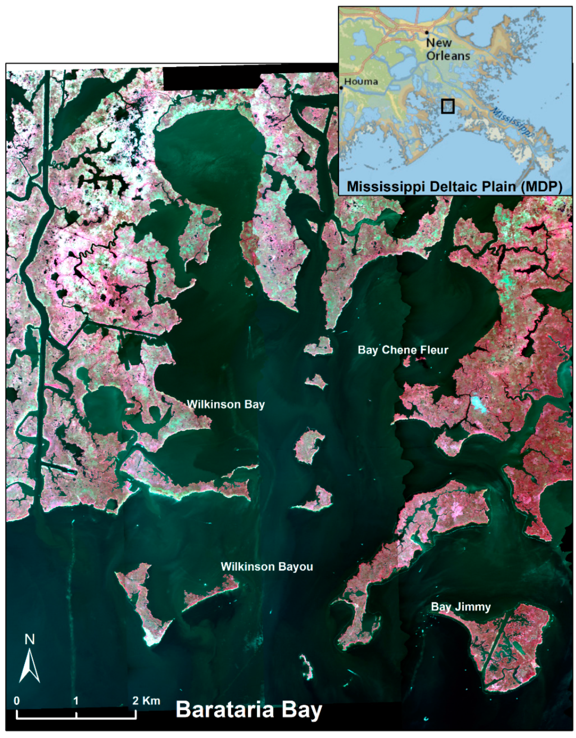
2.1. Study Area

Figure 1 shows the location of Barataria Bay in the Gulf of Mexico along the Louisiana coastline. The bay is in an interlobe basin between the Bird’s Foot Delta and the abandoned Lafourche Delta lobes [42]. It is mainly saltmarsh habitat, as it is cutoff from fresh water or sediment input due to levees along the Mississippi River and the closure of Bayou Lafourche. The dominant vegetation in the low intertidal saltmarshes is Spartina alterniflora (saltmarsh cordgrass) and Juncus roemerianus (needlegrass rush), with subdominants Spartina patens (salt meadow cordgrass), Distichlis spicata (saltgrass) and Batis maritima (saltwort), which are more common in the higher marsh [43]. The DWH oil spill occurred offshore, about 160 km away from Barataria Bay. The oil came in with the tides primarily contaminating the seaward edges of these marshes, and the impact of oil in most areas extended approximately 15 m inland from the shore [31]. The impacted area next to the shoreline is mainly dominated by S. alterniflora and J. roemerianus [31]. The spill started on 20 April 2010 and continued until the well was capped on 15 July 2010. There were confirmed reports of oil in Barataria Bay by 7 July 2010 [44], and most of the oil had already arrived by August before our September image acquisition [39]. Hurricane Isaac made landfall on the Barataria Bay shoreline two years later on 29 August 2012.

2.2. Remote Sensing Data

We used AVIRIS image spectroscopy data collected on 14 September 2010, 15 August 201, and 19 October 2012, with a 3.3-m pixel resolution (86 km2; Figure 1). Image data used in this study are publicly available from the Jet Propulsion Laboratory (JPL) AVIRIS archive (aviris.jpl.nasa.gov). 2010 AVIRIS data were atmospherically calibrated using ACORN 6, Mode 1.5 (ImSpec LLC, Seattle), to apparent surface reflectance. 2011 and 2012 imagery was calibrated by the Jet Propulsion Laboratory before delivery. The 2010 imagery was then georectified to 1-m National Agricultural Imagery Program (NAIP) color infrared images collected in 2010. Finally, the 2011 and 2012 imagery was co-registered to the 2010 imagery using an automated image registration technique [45] that combines robust band-wise compensation for radiometric differences in images [46] with an iterative gradient-based video-sequence alignment method by Irani [47]. Areas of large or systematic change in the scene (e.g., cloud masses, shorelines at different tidal stages or eroded shorelines) were excluded from the image motion estimation. As a result of the image co-registration, the residual pixel misregistration was markedly reduced, allowing more accurate estimates of the changes in the three-year period.
Table 1 summarizes information about each flight line acquisition along with the tidal stage at the time of acquisition. Tidal data were downloaded for the Grand Isle station (tidesandcurrents.noaa.gov) and provide actual water levels recorded, not predicted tides. The water level during the 2010 and 2011 acquisitions is almost identical (4-cm difference). The water level in 2012 is 14 cm lower than in 2011. This could potentially lead to an under-estimation of land lost due to Hurricane Isaac or an over-estimation of recovery due to the exposure of more land. Results will be discussed taking this into consideration.
Images for all three years were classified into six land cover classes: water, photosynthetic vegetation, oil-free Non-Photosynthetic Vegetation (NPV; stems, senescent and dead plant material), oiled NPV, oil-free soil and oiled soil. We used the oil absorption features at 1700 and 2300 nm to differentiate oiled and oil-free shorelines [31]. To represent the shoreline, we used the boundary between the water class and the other five classes from the September 2010 images, and the resulting shoreline vector was simplified and divided into oiled and oil-free shore fragments (Figure 2A). We chose oil-free shore fragments along the same islands exposed to tidal action to ensure that the inference was not biased due to shoreline direction differences. Indeed, because the oil came in with the tides, it had a greater probability of coming ashore on the south-facing island edges and those closer to the open sea. Similarly, the hurricane impact was also likely greatest on the south-facing edges of islands facing the open seas. Thus, by chance alone, we were likely to find greater impact of the hurricane along shores that had been affected by oil than other shores.
To avoid the bias, we generated sites randomly along the oiled and oil-free shore fragments at, on average, a 60-m distance from the centroid of any other site. This resulted in 644 total sites (oiled and oil-free) for 2010, 536 sites in common with 2010 for 2011 and 505 sites in common with both 2010 and 2011 for 2012 (Table 2). Since the DWH oil spill created a zone of dead vegetation, approximately 14 m to 17 m wide along the oiled shoreline [31], each site was buffered by a circle of 20 m in radius and included approximately 115 pixels (Figure 2B).

2.3. Measuring Impact: Vegetation Indices and Land Cover Change

Our earlier analyses showed that oil impacts were significant in September 2010, but there was considerable recovery by August 2011 [31]. In this study, we chose the same vegetation indices to further explore the cumulative impact of the oil spill and Hurricane Isaac in Barataria Bay oiled and oil-free shores. Changes in vegetation productivity, pigment content and water stress, as measured by these indices, are indicators of whether the photosynthetic capacity or phenology of the vegetation is changing [26,31,48,49]. Table 2 describes the indices used and the vegetation characteristics they track.
The index value for a site for a certain year was calculated as the mean of that index for “land” pixels within the site for that year. This is because difference indices, like NDVI or NDII, while meaningful for soil, dry vegetation and green vegetation land cover types, deteriorate to pure noise in water pixels. Therefore, there could be a different number of pixels included per site per year for the index mean calculation. Despite the drawbacks of this approach, we preferred it over using pixels that remained land through all three years because the number of land pixels would be reduced considerably in many sites by the third year.
For each site, we also calculated the fraction of a site covered by either of three land cover types: water (wat), green vegetation (gveg) and soil and non-photosynthetic vegetation (snpv). This calculation used the outputs from the classification of three imagery periods, and we calculated the fractional change in each land cover type over one-year time steps (Table 3). The rate of land cover conversion gives a measure of land loss, from land to water, or of vegetation loss, from green vegetation to senescent (i.e., vegetation that is stressed or undergoing phenological changes) and dying vegetation to soil to water [49,50], but also of vegetation expansion, from soil and non-photosynthetic vegetation or water to green vegetation.

2.4. Comparison Methods for Cumulative Impact of Oil and Hurricane on Vegetation

In September 2010, post-spill vegetation showed signs of stress, senescence and mortality, which were measured using the indices and change metrics described in Table 3. By 2011, recovery was detected when there was an increase in the value of vegetation indices and an increase in the green vegetation fraction in the affected areas [31].
When comparing indices across oiled and oil-free sites, we used the non-parametric Kruskal–Wallis test [55]. Within groups, the index data were not normally distributed, frequently showing skewed or multimodal distributions, due to the presence of green and dying vegetation in oiled pixels (Figure 3). Parametric tests can be robust for skewed data and moderate deviations from normality, but are affected by kurtosis [56]. The Kruskal–Wallis test [55] is insensitive to both skewness and kurtosis [56] and can be used as a measure of the difference between group medians as long as the two distributions being compared have similar variances and distributions [57]. Figure 3 shows that this is true for our between-group comparisons. Hence, a significant p-value indicates that the median index value was significantly different between oiled and oil-free sites, while the sign of the difference shows the direction of change.
Land cover or change metrics were compared using a generalized linear model (GLM) with a logit link function [58,59]. Proportion data, such as change metrics or land cover metrics, do not exhibit the same variance for the mean across the entire range of possible values. As the mean value approaches 0% or 100% cover, variance tends to zero, while it is maximum near a mean of 50% [60,61]. Classic tests, such as Student’s t-test or ANOVA, assume equal within-group variances and their independence of the group mean, whereas the logit link function naturally models the change in variance across the range of the mean values (i.e., 0% and 100% [58,59]). Hence, this method is appropriate and recommended for such data analyses [60]. The model reports the significance of the slope and intercept for each comparison.
A significant slope indicates that the dependent land cover or change metric is significantly different between the two groups of sites (e.g., oiled vs. oil-free, treated vs. untreated, etc.), while the sign of the slope indicates the direction of change. A significant intercept indicates that there is a remnant value of the metric that is not related to group membership. For example, since every site was centered around a point on the shoreline edge, it was likely to have half its pixels as water (see Figure 2). Thus, the metric measuring “percent cover of water” at a site often had a significant intercept.
In addition to site-based comparisons, we also estimated green vegetation and land loss along the entire affected shoreline (oiled and oil-free) in Barataria Bay after Hurricane Isaac. We quantified the number of pixels that transitioned from green vegetation to soil, NPV or open water between 2010 and 2011. This comparison was done zone-to-zone (bands of pixels away from the shore by the same distance), i.e., the zone of the first pixel next to the shore was compared between oiled and oil-free shores, then the pixel-zone next to the shoreline pixels, and so on, until the maximum inland extent of the oil is reached. We expected the maximum impact at the shoreline and decreasing impact as we moved further inland.

2.5. Effect of Site Characteristics on Vulnerability to Disturbances

Several studies have shown that the physical characteristics of the impacted site can have an influence on the effect of both oil-spills and hurricanes [5,6,62]. We hypothesized that shores of narrow land masses were likely to be more susceptible to erosion and show slower recovery compared to shores of wider islands. To test this hypothesis, we divided our sites into narrow and wide sites, where a site along a shore less than 50 m wide was considered a narrow site. Since there were many fewer narrow sites compared to wide sites, we randomly selected 50 sites from more than 250 wide sites to test against the narrow sites. We determined whether oiled narrow sites showed greater land loss and vegetation stress relative to oiled wide sites by comparing indices using the Kruskal–Wallis test and land cover and change metrics using the GLM test as described in Section 2.4.
Between September 2010 and August 2011, several sites were identified as treated by cleanup crews using multiple treatment methods. We did not have data on the kind of treatment performed at each site, but we did have access to information on whether a site was treated or not [63]. We hypothesized that oiled sites that were treated would likely show better recovery in 2011 and less land loss in 2012 as a result of the hurricane. We compared 173 treated sites to 138 sites that were not treated. Treatment was carried out in the years 2010 to 2011 before the 2011 imagery was acquired. The post-oil management actions were geared towards salt marsh recovery and included marsh cleanup actions. Most of the marsh oiling occurred in Louisiana (94.8%), and treatment was customized to specific shoreline segments (71 km out of 796 km of affected marshes) [63]. Cleanup activities were terminated when there was no visible flushable oil, no release of sheens and no thick oil (>1 cm) was detected on the marsh. Natural attenuation was often recommended to avoid further damage to the marshes [63]. We tested whether untreated oiled sites showed greater land loss and vegetation stress relative to treated oiled sites by comparing indices using the Kruskal–Wallis test and land cover and change metrics using the GLM test as described in Section 2.4.

3. Results

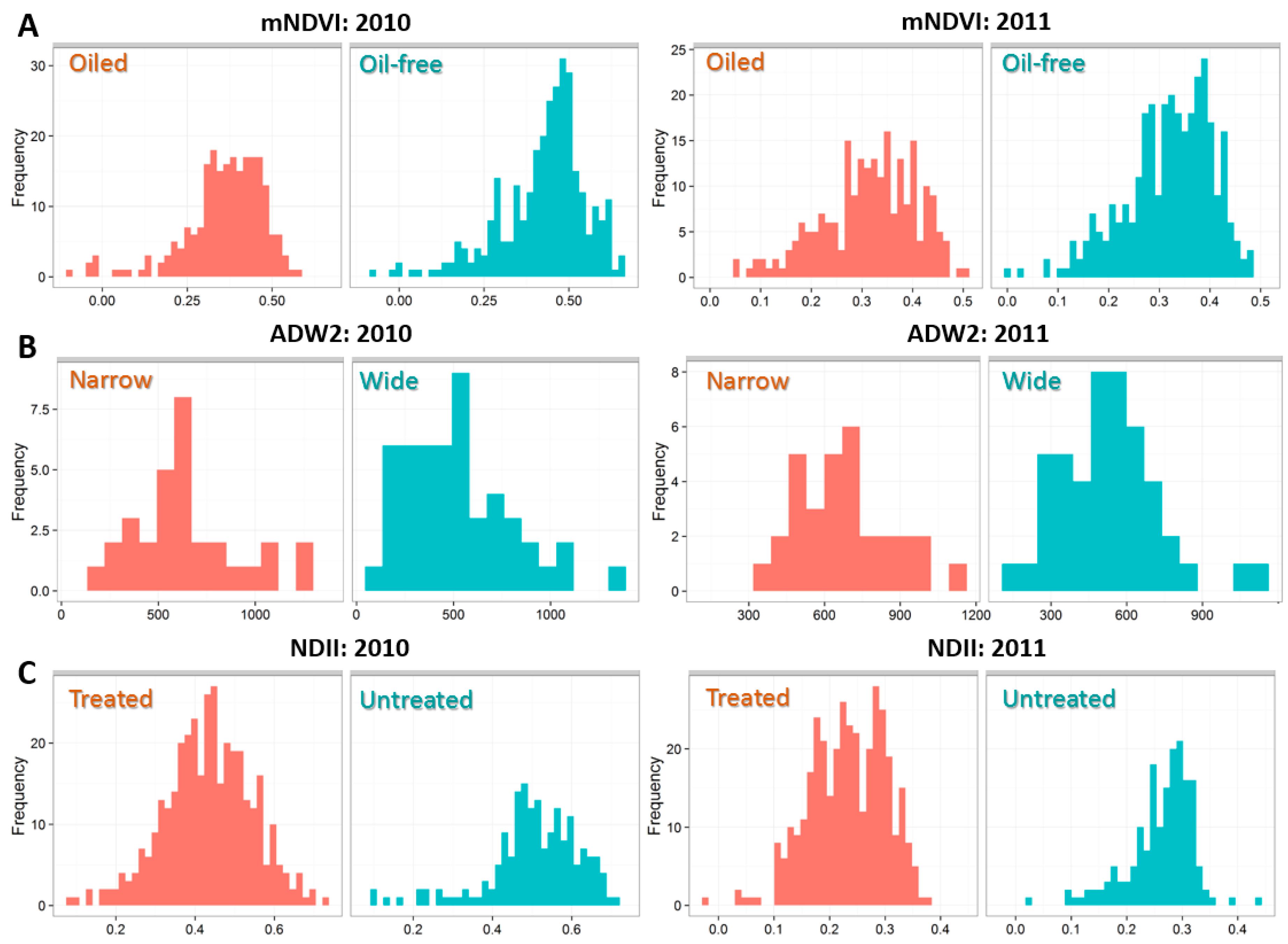
3.1. Cumulative Impact of Oil and Hurricane on Vegetation Indices

In September 2010, land pixels were significantly more stressed in oiled sites relative to oil-free sites. This pattern was observed across all six indices, which showed median and average index values significantly higher for oil-free pixels than for oiled pixels (Table 4). In August 2011, the between-group difference in index values became statistically non-significant (with the exception of mNDVI11p-value = 0.012). In other words, index values in oiled and oil-free sites became more similar in 2011 suggesting some recovery (Table 4). In October 2012, after the hurricane, five of the six indices again showed significant differences in value between oiled and oil-free sites suggesting that recovery was pushed back by the hurricane. All five indices exhibited lower values in oiled sites relative to oil-free sites; however, the difference between the medians was smaller (Table 4: difference in medians).

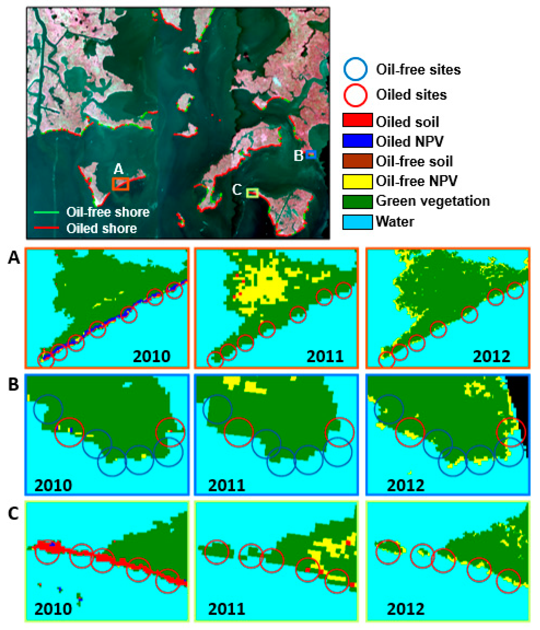
3.2. Cumulative Impact of Oil and Hurricane on Land Cover

In 2010, land cover metrics were significantly different between oiled and oil-free sites, with oiled sites having significantly fewer green vegetation pixels and higher soil/NPV pixels compared to oil-free sites (Table 5). The change in green vegetation and soil/NPV from 2010 to 2011 was significantly different between oiled and oil-free sites. In oiled sites, there was a reduction in soil/NPV pixels, which likely greened up, leading to an increase in green vegetation pixels. In 2012, post hurricane, there was a significant loss of green vegetation pixels to water and soil/NPV in both oiled and oil-free sites. Although all sites showed loss of green vegetation, in oiled sites, the loss was evenly divided between conversion to soil/NPV (Δsnpv_11_12 = 8.8%) or water (Δwat_11_12 = 8.7%). In oil-free sites, most of the green vegetation converted to soil/NPV (Δsnpv_11_12 = 12.1%) rather than water (Δwat_11_12 = 3.4%).

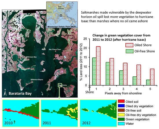
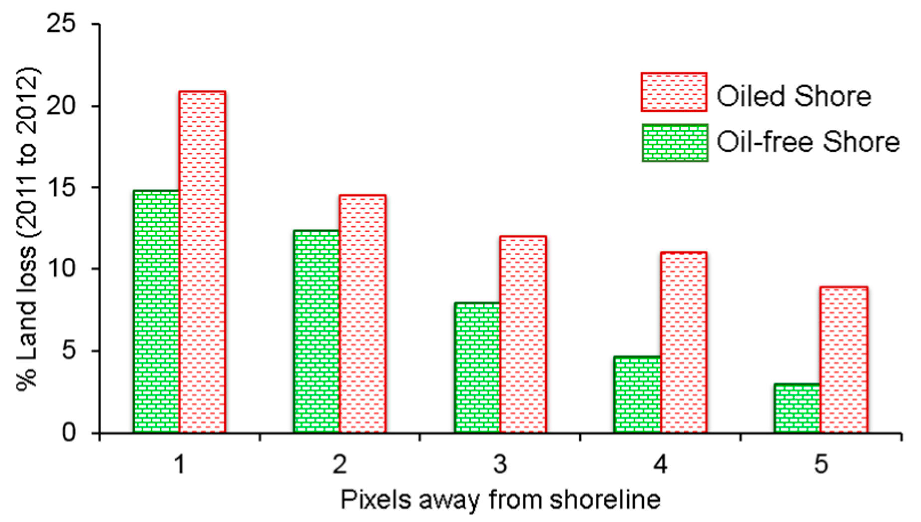
3.3. Zone-Wise Impact Moving Inland from the Shore between Oiled and Oil-Free Shores

The analysis of oiled and oil-free shorelines by zone also confirms the disproportionate impact of the hurricane in oiled areas. While Hurricane Isaac caused shoreline erosion across the entire Barataria Bay in the first 14 to 17 m along the shore, in every zone (n pixels away from shore), the oiled shorelines lost more land than oil-free shorelines (Figure 4). In the first two pixels along the shore (0 to 7 m from the shore), oil-free shorelines lost 13.6% of their land; however, oiled shorelines lost 17.8% of land. Land loss decreased further inland from the shore. In the next two pixels along the shore (7 to 14 m from the shore), the oil-free shorelines lost only 6.3% of their land, while oiled shorelines lost 11.6% of their land (Figure 5).

3.4. Effect of Landmass on Vulnerability to Impact

For all six indices, values in narrow oiled sites were significantly lower than wide sites in 2010 and continued to show a similar pattern in 2011, with the exception of mNDVI (Table 6). In 2012, four of the six indices still showed narrow sites with significantly lower index values relative to wide sites.
Narrow oiled sites had significantly fewer green pixels and more water pixels than wide sites (Table 7). In 2011, narrow and wide sites again differ significantly in green vegetation and water pixels; however, none of the change metrics show any significant difference between the two groups. The 2012 pattern mimics those of 2010 and 2011, showing significant differences only in green vegetation and water pixels, but no significant differences in any of the change metrics.

3.5. Effect of Post-Oil Treatment on Vulnerability to Impact

While post-treatment comparisons are meaningful only for 2011 and 2012 data, we present the 2010 data here to emphasize that the treated and untreated sites were significantly different even before the treatment was applied. The treated sites had significantly lower index values for five of the six indices (Table 8) and significantly less green vegetation and more soil/NPV pixels relative to the untreated sites (Table 9). This might indicate that heavily-impacted shores were more likely to be treated than moderately and lightly affected shores.
Furthermore, our results show that the treated sites experienced a significantly greater conversion from soil/NPV to green vegetation relative to untreated sites (treated: Δgveg_10_11 = 23.8, Δsnpv_10_11 = −21.7, untreated: Δgveg_10_11 = 18.4, Δsnpv_10_11 = −16), thus suggesting that treated sites did recover better than untreated ones. Results from the index value comparisons were more ambiguous. Only two indices showed a significant difference between treated and untreated sites. ARED indicated a slight greening up of land pixels (negative difference in medians, p-value < 0.01), while ADW2 indicated that there was still a water deficit in the recovering plants (positive difference in medians, p-value = 0.02).
In 2012, however, the treated sites showed greater loss of green vegetation and had more soil/NPV pixels relative to untreated sites. Furthermore, all indices showed significantly lower values in treated sites compared to untreated sites indicating more stressed vegetation.

4. Discussion

The impact of hurricanes on subsiding wetlands, such as the saltmarshes of Louisiana, can be beneficial due to sediment accretion in some areas [5,7], but detrimental in areas vulnerable to massive erosion and land loss [11,12,16]. Along shorelines that were affected by the DWH oil spill in 2010, we found that the overarching effect of Hurricane Isaac was loss of green vegetation and of land mass in the first several pixels along the shore.

4.1. Cumulative Effect of Oil Contamination and Hurricane Isaac

This study suggests that there is a cumulative effect of oil and hurricane stress. We observed that vegetation index values in oiled and oil-free sites became more similar in 2011 compared to 2010, suggesting some recovery consistent with the analysis of Khanna et al. [31]. However, after Hurricane Isaac in October 2012, index values again became more dissimilar between oiled and oil-free sites.
Oil coating causes vegetation stress, damaging the canopy and ultimately changing leaf color and leading to vegetation mortality [64]. The spectral resolution of imaging spectroscopy is sufficient to enable discrimination between healthy and stressed vegetation and to monitor the impact of oil contamination [26]. Oil coating may affect the ability of plants to photosynthesize, which can be measured as a shift towards shorter wavelengths of the “red edge” (ca. 700 nm) due to decreased chlorophyll concentration [65]. The loss of photosynthetic ability can decrease the leaf area index, resulting in decreased scattering between leaves [24]. Oil coating can also increase plant stress by altering the water balance and water exchange capacity of the leaves [4]. Our results suggest that in the case of the DWH oil spill, oil coating affected both the photosynthetic capacity of the plants and its water content. These results can be better understood in conjunction with the change detection results in the next section, which corroborate the loss of green vegetation pixels in 2012 in both oiled and oil-free sites.
After the two disturbances, we found that while both oiled and oil-free shores lost healthy marsh vegetation, oiled areas lost significantly more vegetation than oil-free areas. This is likely because the marshes at the interface between land and water were already fragile due to the effects of oil. In oiled sites, we observed a reduction in soil/NPV pixels from 2010 to 2011, which likely greened up leading to an increase in green vegetation pixels. In 2012, post hurricane, there was a significant loss of green vegetation pixels to water and soil/NPV in both oiled and oil-free sites. Pixels with stressed or dead vegetation are likely to first be converted to water because they lack the vegetation cover that serves to hold onto the bare land. In recent research after the DWH oil spill, Lin et al. [23] reported that heavily oiled marshes had significantly lower soil shear strength, lower sedimentation rates and higher vertical soil surface erosion rates. Further, Silliman et al. [13] showed that oiled areas had almost double the rate of shoreline erosion. Hence, the oiled sites lost more marsh area to water than oil-free sites.
The loss of land occurred in bands along the shore, with losses of 17.8% of land in oiled shores in the first 7 m inland, while non-oiled shores lost 13.6% of land. From 7 to 14 m inland, oiled shores land loss was 11.6%, and the oil-free shorelines lost only 6.3% of their land. Again, this is likely because oil-free shores retained most of their vegetation, which traps the soil and prevents erosion due to hurricanes. The cumulative effect of the hurricane was less pronounced inland where the oil impact was lower [31,66]. Tide levels were lower in the 2012 images, but we do not believe that this significantly affected our results. Lower water levels could potentially show up as a gain in soil/NPV pixels (mudflat) at the expense of water. However, instead, our results show a loss to water, which indicates that the hurricane caused a loss of land, but its extent may be somewhat underestimated.
Other disturbances may have affected the study area during the duration of our study. There was a drought in 2011 which could influence the recovery trajectories in 2011 and 2012. However, while seasonal variations are likely to affect the entire marsh somewhat consistently, both the oil spill (since it came in with the tides) and the hurricane preferentially affect the shoreline more than the inland marsh (Figure 5, 2012 imagery). Plant stress due to drought starts in the marsh interior and moves to the shoreline as observed in 2011 imagery (Figure 5). Since we have selected all of our sites along the shoreline, we believe we are primarily looking at oil and hurricane impacts.

4.2. Effect of Landmass on Vulnerability of Oiled Shores

Our results indicated that narrow oiled sites had significantly less green pixels and more water pixels than wide sites a priori (Table 7). This is simply due to the fact that narrow sites are likely to have more water and less land in the 40 m-diameter circle that constitutes a site because of their narrow structure. While most index values were significantly different between the two groups, change detection metrics were comparable across narrow and wide sites. This suggests that recovery of narrow and wide sites was equivalent (e.g., in both sites, green vegetation increased by more than 20%). However, the significant difference between index values in wide and narrow sites indicates that while narrow sites do not disproportionately lose land relative to wide sites, the vegetation in narrow sites was more stressed relative to wide sites after both the oil spill and the hurricane. This encourages the conclusion that indeed, narrower sites are more vulnerable to oil spill impact and that this is maintained but not necessarily exacerbated after the hurricane.

4.3. Effect of Post-Oil Treatment on the Vulnerability of Oiled Shores

Cleanup of the marsh after the oil spill helped with recovery, but was ineffective in ameliorating hurricane impact. Sites that were treated for the impacts of oil showed some signs of greater recovery relative to untreated sites. However, the recovery rates did not make these sites more resilient to impacts of hurricane Isaac in 2012. Treated sites showed greater conversion of green vegetation to soil/NPV and open water relative to untreated sites. This might be due to two reasons: first, treated sites were originally more severely affected than untreated sites, hence they were more vulnerable, and second, treatment often involves planting new saplings after cleanup, and these saplings might still be vulnerable and unable to survive hurricane-force winds and the resulting storm-surge. Zengel et al. [67] showed that manually-treated sites performed better than mechanical treatment by minimizing the detrimental impacts of intensive treatment. There were large differences in the degree of intervention at different sites, and some treatments worked better than others [67]. We did not have detailed information on the type of treatment applied to each of our treated sites; hence, we could not separately test for the effectiveness of each. It is possible that having both types of treatment sites diluted our ability to detect a strong positive impact of treatment on recovery and resilience.

5. Conclusions

Climate change is likely to increase the intensity of hurricanes [68,69]. At the same time, our continued reliance on oil has led companies to explore more deepwater wells, increasing the danger of large, hard-to-stop oil spills, such as DWH. Our results suggest that the environmental impact escalates when multiple disturbances act in quick succession on sensitive endangered ecosystems.
Remote sensing monitoring techniques are necessary to assess long-term impacts of oil spills and the resilience of the ecosystem to recover from their effects, especially when ecosystems are exposed to multiple natural and anthropogenic disturbances. New AVIRIS imagery was acquired in 2015 over Barataria Bay, and future research will allow assessment of lingering impacts, five years after the spill. It is therefore important to maintain such campaigns to understand the fate of coastal salt marshes under the impacts of multiple disturbances. Ghosh et al. [70] have stressed the need for long-term monitoring of coastal wetlands throughout the year to capture seasonal changes in these ecosystems in order to have a base line to compare to.
No single index or group of indices proved exceptionally good at measuring oil and hurricane impact. Moreover, they only told a part of the story. The land cover and change metrics were essential to understanding the full impact of these disturbances. For example, the indices consistently showed narrow sites as more stressed than wide sites; however, there was no significant difference in their land cover change. This means that hurricane and oil impacts affect the physiological health of plants, but also engineer changes to land cover, and the directionality of the forces that bring oil to shore and of the hurricane may impact land masses differentially. Our results highlight the increased risk to ecosystem health from both disturbances, which can inform better management of important coastal areas as the Mississippi Deltaic Plain.

Acknowledgments

This study was funded by a NASA Terrestrial Ecology grant (#NNX12AK58G). We thank Diane Wickland, program manager for Terrestrial Ecology at NASA, for providing access to the AVIRIS database and to the AVIRIS team for preprocessing support. The AVIRIS data are available at http://aviris.jpl.nasa.gov/data/. We thank George Scheer for systems support.

Author Contributions

Shruti Khanna helped with preprocessing of image data, conceived of and designed the study and wrote the manuscript. Maria J. Santos and Alexander Koltunov provided statistical advice and expertise, edited the manuscript and provided feedback. Kristen D. Shapiro helped with data preprocessing, analysis and editing. Mui C. Lay helped with data preprocessing and analysis. Susan L. Ustin contributed lab resources, provided invaluable advice during the analysis phase and helped with editing the manuscript.

Conflicts of Interest

The authors declare no conflict of interest. The funding agency had no role in the design of the study; in the collection, analyses or interpretation of data; in the writing of the manuscript; and in the decision to publish the results.

Abbreviations

The following abbreviations are used in this manuscript:
ADW1Absorption Depth of Water at 980 nm
ADW2Absorption Depth of Water at 1240 nm
ANOVAANalysis of VAriance
AREDAngle formed at Red
AVIRISAirborne Visible/Infrared Imaging Spectrometer
DWHDeep Water Horizon (oil spill)
GLMGeneralized Linear Models
JPLJet Propulsion Laboratory
MDPMississippi Deltaic Plain
mNDVImodified Normalized Difference Vegetation Index
NASANational Aeronautics and Space Administration
NDIINormalized Difference Infrared Index
NDVINormalized Difference Vegetation Index
NPVNon-Photosynthetic Vegetation

References

  1. Meybeck, M. Global Analysis of River Systems: From Earth System Controls to Anthropocene Syndromes. Philos. Trans. R. Soc. Lond. B Biol. Sci. 2003, 358, 1935–1955. [Google Scholar] [CrossRef] [PubMed]
  2. Smith, V. Eutrophication of freshwater and coastal marine ecosystems a global problem. Environ. Sci. Pollut. Res. 2003, 10, 126–139. [Google Scholar] [CrossRef]
  3. Baumann, R.H.; Day, J.W.; Miller, C.A. Mississippi Deltaic Wetland Survival: Sedimentation Versus Coastal Submergence. Science 1984, 224, 1093–1095. [Google Scholar] [CrossRef] [PubMed]
  4. Ko, J.Y.; Day, J.W. A review of ecological impacts of oil and gas development on coastal ecosystems in the Mississippi Delta. Ocean Coast. Manag. 2004, 47, 597–623. [Google Scholar] [CrossRef]
  5. Cahoon, D.R.; Reed, D.J.; Day, J.W., Jr.; Steyer, G.D.; Roelof, M.B.; Lynch, J.C.; McNally, D.; Latif, N. The Influence of Hurricane Andrew on Sediment Distribution in Louisiana Coastal Marshes. J. Coast. Res. 1995, 21, 280–294. [Google Scholar]
  6. Guntenspergen, G.R.; Cahoon, D.R.; Grace, J.; Steyer, G.D.; Fournet, S.; Townson, M.A.; Foote, A.L. Disturbance and Recovery of the Louisiana Coastal Marsh Landscape from the Impacts of Hurricane Andrew. J. Coast. Res. 1995, 21, 324–339. [Google Scholar]
  7. Reed, D. Patterns of sediment deposition in subsiding coastal salt marshes, Terrebonne Bay, Louisiana: The role of winter storms. Estuaries 1989, 12, 222–227. [Google Scholar] [CrossRef]
  8. Reed, D.J. Sea-level rise and coastal marsh sustainability: Geological and ecological factors in the Mississippi delta plain. Geomo 2002, 48, 233–243. [Google Scholar] [CrossRef]
  9. Blum, M.D.; Roberts, H.H. The Mississippi Delta Region: Past, Present, and Future. AREPS 2012, 40, 655–683. [Google Scholar] [CrossRef]
  10. Blum, M.D.; Roberts, H.H. Drowning of the Mississippi Delta due to insufficient sediment supply and global sea-level rise. Nat. Geosci. 2009, 2, 488–491. [Google Scholar] [CrossRef]
  11. Day, J.; Britsch, L.; Hawes, S.; Shaffer, G.; Reed, D.; Cahoon, D. Pattern and process of land loss in the Mississippi Delta: A Spatial and temporal analysis of wetland habitat change. Estuaries 2000, 23, 425–438. [Google Scholar] [CrossRef]
  12. Day, J.W.; Boesch, D.F.; Clairain, E.J.; Kemp, G.P.; Laska, S.B.; Mitsch, W.J.; Orth, K.; Mashriqui, H.; Reed, D.J.; Shabman, L.; et al. Restoration of the Mississippi Delta: Lessons from Hurricanes Katrina and Rita. Science 2007, 315, 1679–1684. [Google Scholar] [CrossRef] [PubMed]
  13. Silliman, B.R.; van de Koppel, J.; McCoy, M.W.; Diller, J.; Kasozi, G.N.; Earl, K.; Adams, P.N.; Zimmerman, A.R. Degradation and resilience in Louisiana salt marshes after the BP–Deepwater Horizon oil spill. Proc. Natl. Acad. Sci. USA 2012, 109, 11234–11239. [Google Scholar] [CrossRef] [PubMed]
  14. White, W.A.; Tremblay, T.A. Submergence of Wetlands as a Result of Human-Induced Subsidence and Faulting along the upper Texas Gulf Coast. J. Coast. Res. 1995, 11, 788–807. [Google Scholar]
  15. Chabreck, R.H.; Palmisano, A.W. The Effects of Hurricane Camille on the Marshes of the Mississippi River Delta. Ecology 1973, 54, 1118–1123. [Google Scholar] [CrossRef]
  16. Stone, G.W.; Grymes, J.M., III; Dingler, J.R.; Pepper, D.A. Overview and Significance of Hurricanes on the Louisiana Coast, USA. J. Coast. Res. 1997, 13, 656–669. [Google Scholar]
  17. Keen, T.R.; Bentley, S.J.; Chad Vaughan, W.; Blain, C.A. The generation and preservation of multiple hurricane beds in the northern Gulf of Mexico. Mar. Geol. 2004, 210, 79–105. [Google Scholar] [CrossRef]
  18. Stone, G.W.; Liu, B.; Pepper, D.A.; Wang, P. The importance of extratropical and tropical cyclones on the short-term evolution of barrier islands along the northern Gulf of Mexico, USA. Mar. Geol. 2004, 210, 63–78. [Google Scholar] [CrossRef]
  19. Nyman, J.A.; Crozier, C.R.; DeLaune, R.D. Roles and Patterns of Hurricane Sedimentation in an Estuarine Marsh Landscape. ECSS 1995, 40, 665–679. [Google Scholar] [CrossRef]
  20. Rejmánek, M.; Sasser, C.E.; Peterson, G.W. Hurricane-induced sediment deposition in a gulf coast marsh. Estuar. Coast. Shelf Sci. 1988, 27, 217–222. [Google Scholar] [CrossRef]
  21. Nyman, J.A.; Walters, R.J.; Delaune, R.D.; Patrick, W.H., Jr. Marsh vertical accretion via vegetative growth. Estuar. Coast. Shelf Sci. 2006, 69, 370–380. [Google Scholar] [CrossRef]
  22. Turner, R.E.; Swenson, E.M.; Milan, C.S. Organic and Inorganic Contributions to Vertical Accretion in Salt Marsh Sediments. In Concepts and Controversies in Tidal Marsh Ecology; Weinstein, M.P., Kreeger, D.A., Eds.; Springer Netherlands: Dordrecht, The Netherlands, 2000; pp. 583–595. [Google Scholar]
  23. Lin, Q.; Mendelssohn, I.A.; Graham, S.A.; Hou, A.; Fleeger, J.W.; Deis, D.R. Response of salt marshes to oiling from the Deepwater Horizon spill: Implications for plant growth, soil surface-erosion, and shoreline stability. Sci. Total Environ. 2016, 557–558, 369–377. [Google Scholar] [CrossRef] [PubMed]
  24. Boochs, F.; Kupfer, G.; Dockter, K.; Kuhbauch, W. Shape of the red edge as vitality indicator for plants. Int. J. Remote Sens. 1990, 11, 1741–1753. [Google Scholar] [CrossRef]
  25. Bammel, B.H.; Birnie, R.W. Spectral Reflectance Response of Big Sagebrush to Hydrocarbon-Induced Stress in the Bighorn Basin, Wyoming; American Society for Photogrammetry and Remote Sensing: Bethesda, MD, USA, 1994; Volume 60. [Google Scholar]
  26. Li, L.; Ustin, S.L.; Lay, M. Application of AVIRIS data in detection of oil-induced vegetation stress and cover change at Jornada, New Mexico. Remote Sens. Environ. 2005, 94, 1–16. [Google Scholar] [CrossRef]
  27. Van Der Meer, F.; Van Dijk, P.; Van Der Werff, H.; Yang, H. Remote sensing and petroleum seepage: A review and case study. Terra Nova 2002, 14, 1–17. [Google Scholar] [CrossRef]
  28. Yang, H.; Zhang, J.; Van der Meer, F.; Kroonenberg, S.B. Geochemistry and field spectrometry for detecting hydrocarbon microseepage. Terra Nova 1998, 10, 231–235. [Google Scholar] [CrossRef]
  29. Turpie, K.R. Explaining the Spectral Red-Edge Features of Inundated Marsh Vegetation. J. Coast. Res. 2013, 29, 1111–1117. [Google Scholar] [CrossRef]
  30. Beland, M.; Roberts, D.A.; Peterson, S.H.; Biggs, T.W.; Kokaly, R.F.; Piazza, S.; Roth, K.L.; Khanna, S.; Ustin, S.L. Mapping changing distributions of dominant species in oil-contaminated salt marshes of Louisiana using imaging spectroscopy. Remote Sens. Environ. 2016, 182, 192–207. [Google Scholar] [CrossRef]
  31. Khanna, S.; Santos, M.J.; Ustin, D.S.L.; Koltunov, A.; Kokaly, R.F.; Roberts, D.A. Detection of salt marsh vegetation stress after the Deepwater Horizon BP oil spill along the shoreline of gulf of Mexico using AVIRIS data. PloS ONE 2013, 8, e78989. [Google Scholar] [CrossRef] [PubMed]
  32. Mishra, D.R.; Cho, H.J.; Ghosh, S.; Fox, A.; Downs, C.; Merani, P.B.T.; Kirui, P.; Jackson, N.; Mishra, S. Post-spill state of the marsh: Remote estimation of the ecological impact of the Gulf of Mexico oil spill on Louisiana Salt Marshes. Remote Sens. Environ. 2012, 118, 176–185. [Google Scholar] [CrossRef]
  33. Wang, W.; Qu, J.J.; Hao, X.; Liu, Y.; Stanturf, J.A. Post-hurricane forest damage assessment using satellite remote sensing. Agric. For. Meteorol. 2010, 150, 122–132. [Google Scholar] [CrossRef]
  34. Moss, L. The 13 largest oil spills in history. In Mother Nature Network; Narrative Content Group: Atlanta, GA, USA, 2010. [Google Scholar]
  35. Lin, Q.; Mendelssohn, I.A. Impacts and recovery of the Deepwater Horizon Oil Spill on vegetation structure and function of coastal salt marshes in the northern gulf of Mexico. Environ. Sci. Technol. 2012, 46, 3737–3743. [Google Scholar] [CrossRef] [PubMed]
  36. McClenachan, G.; Turner, R.E.; Tweel, A.W. Effects of oil on the rate and trajectory of Louisiana marsh shoreline erosion. Environ. Res. Lett. 2013, 8, 044030. [Google Scholar] [CrossRef]
  37. Ramsey, E., III; Rangoonwala, A.; Suzuoki, Y.; Jones, C.E. Oil detection in a coastal marsh with polarimetric Synthetic Aperture Radar (SAR). Remote Sens. 2011, 3, 2630–2662. [Google Scholar] [CrossRef] [Green Version]
  38. Kokaly, R.F.; Couvillion, B.R.; Holloway, J.M.; Roberts, D.A.; Ustin, S.L.; Peterson, S.H.; Khanna, S.; Piazza, S.C. Spectroscopic remote sensing of the distribution and persistence of oil from the Deepwater Horizon spill in Barataria Bay marshes. Remote Sens. Environ. 2013, 129, 210–230. [Google Scholar] [CrossRef]
  39. Peterson, S.H.; Roberts, D.A.; Beland, M.; Kokaly, R.F.; Ustin, S.L. Oil detection in the coastal marshes of Louisiana using MESMA applied to band subsets of AVIRIS data. Remote Sens. Environ. 2015, 159, 222–231. [Google Scholar] [CrossRef]
  40. Berg, R. Tropical Cyclone Report: Hurricane Isaac; National Hurricane Center, National Oceanic and Atmospheric Administration: Miami, FL, USA, 2013. [Google Scholar]
  41. Mo, Y.; Momen, B.; Kearney, M.S. Quantifying moderate resolution remote sensing phenology of Louisiana coastal marshes. Ecol. Model. 2015, 312, 191–199. [Google Scholar] [CrossRef]
  42. Wilson, C.A.; Allison, M.A. An equilibrium profile model for retreating marsh shorelines in southeast Louisiana. Estuar. Coast. Shelf Sci. 2008, 80, 483–494. [Google Scholar] [CrossRef]
  43. Gosselink, J.G.; Pendleton, E.C. The Ecology of Delta Marshes of Coastal Louisiana: A Community Profile; U.S. Fish and Wildlife Service: Washington, DC, USA, 1984; p. 156.
  44. Strassmann, M. The Fight over Keeping Oil out of Barataria Bay. Available online: http://www.cbsnews.com (accessed on 7 July 2010).
  45. Koltunov, A.; Ustin, S.L.; Quayle, B.; Schwind, B. GOES Early Fire Detection (GOES-EFD) system prototype. In Proceedings of the ASPRS 2012 Anuual Conference, Sacramento, CA, USA, 19–23 March 2012.
  46. Koltunov, A.; Ben-Dor, E.; Ustin, S.L. Image construction using multitemporal observations and Dynamic Detection Models. Int. J. Remote Sens. 2008, 30, 57–83. [Google Scholar] [CrossRef]
  47. Irani, M. Multi-frame correspondence estimation using subspace constraints. IJCV 2002, 48, 173–194. [Google Scholar] [CrossRef]
  48. Carter, G.A. Responses of Leaf Spectral Reflectance to Plant Stress. Am. J. Bot. 1993, 80, 239–243. [Google Scholar] [CrossRef]
  49. Ozesmi, S.; Bauer, M. Satellite remote sensing of wetlands. Wetlands Ecol. Manag. 2002, 10, 381–402. [Google Scholar] [CrossRef]
  50. Turner, R.E.; Rao, Y.S. Relationships between Wetland Fragmentation and Recent Hydrologic Changes in a Deltaic Coast. Estuaries 1990, 13, 272–281. [Google Scholar] [CrossRef]
  51. Tucker, C.J. Red and photographic infrared linear combinations for monitoring vegetation. Remote Sens. Environ. 1979, 8, 127–150. [Google Scholar] [CrossRef]
  52. Hunt, E.R.; Rock, B.N. Detection of changes in leaf water content using near-infrared and middle-infrared reflectances. Remote Sens. Environ. 1989, 30, 43–54. [Google Scholar]
  53. Gitelson, A.; Merzlyak, M.N. Spectral reflectance changes associated with autumn senescence of Aesculus-hippocastanum L. and Acer-platanoides L. leaves—Spectral features and relation to chlorophyll estimation. J. Plant Physiol. 1994, 143, 286–292. [Google Scholar] [CrossRef]
  54. Nagler, P.L.; Daughtry, C.S.T.; Goward, S.N. Plant litter and soil reflectance. Remote Sens. Environ. 2000, 71, 207–215. [Google Scholar] [CrossRef]
  55. Kruskal, W.H.; Wallis, W.A. Use of Ranks in One-Criterion Variance Analysis. J. Am. Stat. Assoc. 1952, 47, 583–621. [Google Scholar] [CrossRef]
  56. Khan, A.; Rayner, G.D. Robustness to Non-Normality of Common Tests for the Many-Sample Location Problem. J. Appl. Math. Decis. Sci. 2003, 7, 187–206. [Google Scholar] [CrossRef]
  57. McDonald, J.H. The Kruskal-Wallis Test. In Handbook of Biological Statistics; McDonald, J.H., Ed.; Sparky House Publishing Baltimore: Baltimore, MD, USA, 2009; Volume 2, pp. 158–165. [Google Scholar]
  58. McCullagh, P. Generalized linear models. Eur. J. Oper. Res. 1984, 16, 285–292. [Google Scholar] [CrossRef]
  59. Nelder, J.A.; Baker, R.J. Generalized Linear Models. In Encyclopedia of Statistical Sciences; John Wiley & Sons, Inc.: Hoboken, NJ, USA, 2004. [Google Scholar]
  60. Crawley, M.J. The R Book, 2nd ed.; Wiley: West Sussex, UK, 2013; p. 1051. [Google Scholar]
  61. Venables, W.N.; Dichmont, C.M. GLMs, GAMs and GLMMs: An overview of theory for applications in fisheries research. Fish. Res. 2004, 70, 319–337. [Google Scholar] [CrossRef]
  62. Bryant, J.; Chabreck, R. Effects of impoundment on vertical accretion of coastal marsh. Estuaries 1998, 21, 416–422. [Google Scholar] [CrossRef]
  63. Michel, J.; Owens, E.H.; Zengel, S.; Graham, A.; Nixon, Z.; Allard, T.; Holton, W.; Reimer, P.D.; Lamarche, A.; White, M.; et al. Extent and degree of shoreline oiling: Deepwater Horizon oil spill, Gulf of Mexico, USA. PLoS ONE 2013, 8, e65087. [Google Scholar] [CrossRef] [PubMed]
  64. Leifer, I.; Lehr, W.J.; Simecek-Beatty, D.; Bradley, E.; Clark, R.; Dennison, P.; Hu, Y.; Matheson, S.; Jones, C.E.; Holt, B.; et al. State of the art satellite and airborne marine oil spill remote sensing: Application to the BP Deepwater Horizon oil spill. Remote Sens. Environ. 2012, 124, 185–209. [Google Scholar] [CrossRef]
  65. van der Meijde, M.; van der Werff, H.M.A.; Jansma, P.F.; van der Meer, F.D.; Groothuis, G.J. A spectral-geophysical approach for detecting pipeline leakage. IJAEO 2009, 11, 77–82. [Google Scholar] [CrossRef]
  66. Kokaly, R.F.; Heckman, D.; Holloway, J.; Piazza, S.; Couvillion, B.; Steyer, G.D.; Mills, C.; Hoefen, T.M. Shoreline Surveys of Oil-Impacted Marsh in Southern Louisiana, July to August 2010; U.S. Geological Survey: Reston, VA, USA, 2011; p. 124.
  67. Zengel, S.; Bernik, B.M.; Rutherford, N.; Nixon, Z.; Michel, J. Heavily Oiled Salt Marsh following the Deepwater Horizon Oil Spill, Ecological Comparisons of Shoreline Cleanup Treatments and Recovery. PLoS ONE 2015, 10, e0132324. [Google Scholar] [CrossRef] [PubMed]
  68. Easterling, D.R.; Meehl, G.A.; Parmesan, C.; Changnon, S.A.; Karl, T.R.; Mearns, L.O. Climate Extremes: Observations, Modeling, and Impacts. Science 2000, 289, 2068–2074. [Google Scholar] [CrossRef] [PubMed]
  69. Lambert, S.J.; Fyfe, J.C. Changes in winter cyclone frequencies and strengths simulated in enhanced greenhouse warming experiments: Results from the models participating in the IPCC diagnostic exercise. ClDy 2006, 26, 713–728. [Google Scholar] [CrossRef]
  70. Ghosh, S.; Mishra, D.R.; Gitelson, A.A. Long-term monitoring of biophysical characteristics of tidal wetlands in the northern Gulf of Mexico—A methodological approach using MODIS. Remote Sens. Environ. 2016, 173, 39–58. [Google Scholar] [CrossRef]
Figure 1. Color-infrared AVIRIS imagery acquired in September 2010 over Barataria Bay in the Gulf of Mexico.
Remotesensing 09 00169 g001
Figure 2. Grey-scale Normalized Difference Vegetation Index image of Barataria Bay showing (A) oiled (red) and oil-free (blue) shore fragments and (B) a small section showing the selection of sites (green circles) along the shore fragments.
Remotesensing 09 00169 g002
Figure 3. Histograms of index values from 2010 and 2011 shown to illustrate that the distributions were comparable across groups. Panels show index value histograms for (A) oiled and oil-free groups, (B) narrow and wide groups and (C) treated and untreated groups.
Remotesensing 09 00169 g003
Figure 4. Percentage land loss in 2010 compared to 2011 for all oiled vs. oil-free sites
Remotesensing 09 00169 g004
Figure 5. Color infrared imagery of Barataria Bay showing oiled and oil-free shores and the location of three insets, (A) moderately oiled island shoreline, (B) lightly oiled big island shoreline and (C) heavily oiled narrow land strip and island shore. The row images show classification results for all three years (2010, 2011 and 2012) for each inset and the distribution of oiled/oil-free sites within it. Severely oiled dead and dying vegetation pixels in 2010 show greening in 2011, but are vulnerable to loss after the hurricane in 2012. Panel (C) also shows the greater loss of vegetation in narrow sites relative to wide sites.
Remotesensing 09 00169 g005
Table 1. Date and time of image acquisitions for all three years and water level at the time of collection.
Time (GMT)Flight DatePixel Resolution (m)Number of Flight LinesTide Level at Time of Image (m)
18:5714 September 20103.5 × 3.540.21
16:1415 August 20117.7 × 7.720.25
15:0619 October 20123.3 × 3.340.11
Table 2. Total number of sites selected along oiled and oil-free shores in 2010, 2011 and 2012. Sites were chosen in subsequent years only if they were selected in previous years. Oiled sites were further described as narrow (a small strip of land along the shoreline) or wide (a larger wetland area going deep into the interior beyond the intertidal zone), treated (for oil contamination) or untreated.
201020112012
oiled311311290
narrow323227
wide505050
treated173173165
untreated138138125
oil-free225225215
Table 3. Indices and land cover and change metrics calculated for each site along with their description, citations, and formulae.
VariablesDescription
IndicesNDVI10/11/12Normalized Difference Vegetation Index: tracks vegetation health, pigment and abundance [51]
NDII10/11/12Normalized Difference Infrared Index: tracks plant health and water content [52]
ARED10/11/12Angle at Red: tracks change in land cover and photosynthetic pigment [31]
mNDVI10/11/12Modified NDVI or red-edge NDVI: sensitive to change in vegetation health, pigment and abundance [53]
ADW110/11/12Absorption Depth of Water at 980 nm: sensitive to plant water content [31,54]
ADW210/11/12Absorption Depth of Water at 1240 nm: sensitive to plant water content [31,54]
Land Cover/Change Metricspveg_10/11/12Number of green vegetation pixels at each site for each year/total pixels at each site for each year (%)
psnpv_10/11/12Number of dry vegetation pixels at each site for each year/total pixels at each site for each year (%)
pwat_10/11/12Number of water pixels at each site for each year/total pixels at each site for each year (%)
Δgveg_10_11pveg_11-pveg_10 1
Δgveg_11_12pveg_12-pveg_11
Δwat_10_11pwat_11-pwat_10
Δwat_11_12pwat_12-pwat_11
Δsnpv_10_11psnpv_11-psnpv_10
Δsnpv_11_12psnpv_12-psnpv_11
1 “-“ indicates subtraction.
Table 4. Analysis of variance using the Kruskal–Wallis test between oiled and oil-free sites for indices calculated on all land pixels for all three years. p-values in bold are significant at the 0.05 significance level.
MeanStandard DeviationDifferenceKruskal–Wallis
IndexOiledOil-FreeOiledOil-Freein MediansHp-Value
NDVI100.5270.6270.1380.1250.090102.36<0.0001
NDII100.4220.5030.1130.1060.08174.90<0.0001
ARED104.7955.2040.5440.3710.38577.93<0.0001
mNDVI100.3560.4570.1200.1130.098107.00<0.0001
ADW110293.8365.5126.9107.481.251.80<0.0001
ADW210606.2701.2264.5221.3129.529.52<0.0001
NDVI110.5310.5390.1090.0940.0070.120.7275
NDII110.3180.3170.0930.083−0.0040.240.6263
ARED110.8680.7950.3660.266−0.0502.710.0998
mNDVI115.0945.0500.4350.332−0.0936.270.0123
ADW111404.6389.2141.2125.6−16.80.900.3416
ADW211643.8653.5177.2146.718.40.650.4219
NDVI120.3100.3570.1690.1200.0326.770.0093
NDII120.5280.5160.1360.120−0.0322.210.1373
ARED123.9584.0400.4900.3800.0794.380.0365
mNDVI120.2070.2440.1320.0990.0356.850.0089
ADW112134.8147.058.650.011.44.190.0407
ADW212465.8503.7156.9137.321.44.620.0315
Table 5. GLM results using the binomial model for oiled vs. oil-free sites for land cover change metrics calculated for all sites. p-values in bold are significant at the 0.05 significance level.
Land CoverMeanStandard DeviationSlopeIntercept
Change MetricOiledOil-FreeOiledOil-FreeZ-Valuep-ValueZ-Valuep-Value
pveg_1036.3150.8514.8815.44−8.87<0.0019.57<0.001
pwat_1043.1046.9613.2115.43−2.970.0034.24<0.001
psnpv_1020.582.2411.123.8410.75<0.001−9.95<0.001
pveg_1157.6957.6821.4020.690.010.9921.650.100
pwat_1140.8941.9721.4720.68−0.560.5732.690.007
psnpv_111.380.364.801.592.570.0103.88<0.001
Δgveg_10_1121.396.8322.5819.076.87<0.001−0.120.905
Δwat_10_11−2.22−4.9919.4018.551.600.1095.01<0.001
Δsnpv_10_11−19.20−1.8812.154.34−10.69<0.001−8.89<0.001
pveg_1240.2642.2022.5821.54−0.960.3353.120.002
pwat_1249.5645.3622.3619.082.180.030−0.070.944
psnpv_1210.2112.497.699.00−3.000.0035.190.001
Δgveg_11_12−17.43−15.4819.8916.85−1.150.2512.880.004
Δwat_11_128.673.4020.4416.153.030.0023.63<0.001
Δsnpv_11_128.8312.138.968.67−3.98<0.0015.99<0.001
Table 6. Kruskal–Wallis test results for narrow vs. wide oiled sites for indices calculated on all land pixels for all three years. p-values in bold are significant at the 0.05 significance level.
MeanStandard DeviationDifferenceKruskal–Wallis
IndexWideNarrowWideNarrowIn MediansHp-Value
NDVI100.5450.3720.1210.176−0.14135.81<0.0001
NDII100.4270.3770.1090.131−0.0755.290.0215
ARED104.8354.4420.4840.850−0.3055.730.0167
mNDVI100.3720.2190.1050.150−0.14031.70<0.0001
ADW110305.6191.1121.6128.0−116.719.05<0.0001
ADW210626.4430.5261.5225.8−160.816.380.0001
NDVI110.5410.4300.1030.123−0.08523.39<0.0001
NDII110.3250.2530.0900.097−0.06814.620.0001
ARED110.8361.1770.3350.4960.20918.48<0.0001
mNDVI115.0915.1180.4440.350−0.0020.000.9843
ADW111412.8326.0135.8168.9−98.213.450.0002
ADW211660.1487.3167.6193.2−186.325.01<0.0001
NDVI120.3310.1140.1500.221−0.23627.78<0.0001
NDII120.5270.5340.1360.1350.0600.260.6077
ARED123.9613.9260.4980.4070.0540.090.7706
mNDVI120.2210.0660.1190.169−0.17622.71<0.0001
ADW112138.0103.558.451.5−37.08.620.0033
ADW212482.3305.0146.8163.6−210.123.38<0.0001
Table 7. GLM results using the binomial model for narrow vs. wide oiled sites for land cover change metrics calculated for all sites. p-values in bold are significant at the 0.05 significance level.
Land CoverMeanStandard DeviationSlopeIntercept
Change MetricNarrowWideNarrowWideZ-Valuep-ValueZ-Valuep-Value
pveg_1019.6538.1513.8813.315.73<0.001−2.320.021
pwat_1059.3241.3111.8713.84−6.17<0.0017.67<0.001
psnpv_1021.1020.5211.1511.03−0.280.7835.71<0.001
pveg_1140.7159.5820.4322.784.35<0.0010.250.799
pwat_1159.0638.8820.3822.79−4.59<0.0017.62<0.001
psnpv_110.261.505.031.441.170.24010.96<0.001
Δgveg_10_1121.0621.4322.9419.420.080.9338.44<0.001
Δwat_10_11−0.26−2.4319.7715.82−0.590.55411.58<0.001
Δsnpv_10_11−20.84−19.0112.2711.010.790.4276.61<0.001
pveg_1219.6142.5521.9717.104.94<0.0012.090.037
pwat_1270.5247.2421.5019.06−5.07<0.0017.84<0.001
psnpv_129.9410.247.796.830.210.8366.89<0.001
Δgveg_11_12−21.10−17.0320.1417.401.080.2798.62<0.001
Δwat_11_1211.458.3620.9415.26−0.800.42410.55<0.001
Δsnpv_11_129.688.739.147.20−0.560.5778.28<0.001
Table 8. Kruskal–Wallis test results for treated vs. untreated oiled sites for indices calculated on all land pixels for all three years. p-values in bold are significant at the 0.05 significance level.
MeanStandard deviationDifferenceKruskal–Wallis
IndexTreatedUntreatedTreatedUntreatedIn MediansHp-Value
NDVI100.5270.5280.1180.1600.0192.030.1544
NDII100.4020.4470.1000.1230.05515.740.0001
ARED104.6924.9230.4920.5800.39420.44<0.0001
mNDVI100.3440.3710.1060.1340.05410.020.0015
ADW110266.5328.1107.0141.282.720.31<0.0001
ADW210543.4684.9219.4294.4136.719.09<0.0001
NDVI110.5210.5430.1130.1040.0233.060.0804
NDII110.3130.3250.0940.0920.0121.520.2174
ARED110.9300.7890.4080.287−0.1228.520.0035
mNDVI115.0545.1440.4910.3470.0220.530.4682
ADW111394.5417.4136.8146.229.32.430.1188
ADW211622.8670.7184.8163.762.65.450.0196
NDVI120.2800.3510.1690.1610.05518.50<0.0001
NDII120.5140.5470.1400.1280.0445.420.0199
ARED123.8324.1230.4280.5170.43929.62<0.0001
mNDVI120.1760.2470.1320.1220.06825.40<0.0001
ADW112122.3151.356.058.029.317.75<0.0001
ADW212435.5505.8147.7160.373.616.68<0.0001
Table 9. GLM results using the binomial model for treated vs. untreated oiled sites for land cover change metrics calculated for all sites. p-values in bold are significant at the 0.05 significance level.
Land CoverMeanStandard DeviationSlopeIntercept
Change MetricTreatedUntreatedTreatedUntreatedZ-Valuep-ValueZ-Valuep-Value
pveg_1034.1738.9814.5414.91−2.800.0053.31<0.001
pwat_1042.1844.2612.6413.85−1.380.1681.890.059
psnpv_1023.6716.7010.5910.585.28<0.001−3.98<0.001
pveg_1157.9657.3621.5821.250.240.8070.460.646
pwat_1140.1041.8821.5321.43−0.730.4681.560.119
psnpv_111.960.655.812.982.210.0271.200.230
Δgveg_10_1123.7918.3822.1722.822.090.0370.000.997
Δwat_10_11−2.08−2.3818.0921.000.140.8911.980.047
Δsnpv_10_11−21.71−16.0412.5810.83−3.99<0.001−2.450.014
pveg_1238.2342.8221.3623.86−1.780.0752.500.013
pwat_1250.8048.0121.5323.351.090.274−0.190.850
psnpv_1211.019.207.857.392.040.041−0.470.641
Δgveg_11_12−19.73−14.5417.4022.36−2.260.024−0.030.977
Δwat_11_1210.706.1318.9621.971.950.0521.070.286
Δsnpv_11_129.058.559.907.650.490.6281.070.284

