Fast Detection of Oil Spills and Ships Using SAR Images

Abstract

In this paper, we show the capabilities of a new maritime control system based on the processing of COSMO-SkyMed Synthetic Aperture Radar (SAR) images. This system aims at fast detection of ships that may be responsible for illegal oil dumping. In particular, a novel detection algorithm based on the joint use of the significance parameter, wavelet correlator and a two-dimensional Constant False Alarm Rate (2D-CFAR) is designed. Results show the effectiveness of such algorithms, which can be used by the maritime authorities to have a faster although still reliable response. The proposed algorithm, together with the short revisit time of the COSMO-SkyMed constellation, can help with tracking the scenario evolution from one acquisition to the next.

1. Introduction

Ocean pollution due to oil slicks remains a major environmental hazard. Oil tanker accidents (such as Exxon Valdez, Erika and Prestige) only account for 5% of total oil pollution worldwide, as 95% of that comes from illegal discharges [1]. In the Mediterranean Sea, oil pollution monitoring is normally carried out by aircraft or ships. This is expensive and is constrained by the limited availability of these resources. In order to provide all-weather and global monitoring of such events, spaceborne Synthetic Aperture Radar (SAR) has been recognized as a cornerstone. At present time, for example, the European Maritime Safety Agency (EMSA) [2] is already using SAR imagery for oil spill and ship detection. Satellite imagery can provide a significant contribution in this field, identifying probable spills and tracking ships’ routes over very large areas, then guiding aerial surveys for precise observations on specific locations. Automatic detection and classification of oil spills in SAR images has been widely researched. State-of-the-art research in this topic covers several aspects of the observation of oil spills and ship detection. A fertile field is represented by the use of radar polarimetry to detect and classify oil spills. Migliaccio et al. [3] explored thoroughly the problem concluding that polarimetric features’ extraction helps greatly in the detection and classification of oil spills and look-alikes using eigenvector-eigenvalues decomposition [4]. Moreover, they also introduced the concept of polarimetric wavelet for sea analysis and the concept of speckle characterization for dark areas’ differentiation [5,6]. Furthermore, Shirvany et al. [7] proposed a method that makes use of radar polarimetry to detect oil spill and ships, using the degree of polarization (lower for spills, higher for ships). Again, Migliaccio et al. [8] proposed a method of ship identification with very high resolution (tenth of a meter) Single Look Complex (SLC) SAR non-polarimetric images, actively using speckle and the dominant scattering behavior of the ship. Unfortunately, often, polarimetric data are not available, and the resolution of the images is not so high (for example, in StripMap images, the resolution is no more than 3 m). In this paper, we propose a method of fast oil spill and ship detection for non-polarimetric StripMap SAR imagery, apt to process large datasets in the order of tens of minutes, and to correlate possible responsible ships with detected oil spills. Data from the COSMO-SkyMed (CSK) constellation are particularly appropriate because of the relatively short revisiting time (down to 2.5 h). In this paper, we focus on the fast detection of elements of interests, without however going in depth toward the analysis of all of the features usually studied in oil spill detection, such as aging, wind effects and oil types, which are not the scope of this article. First, the fractal model of the sea is explained and how a reduced set of parameters estimated from this model can help to classify an oil spill out of seas images. Then, an automatic segmentation algorithm to detect the areas with the weakest radar return level is shown. These areas are then classified as oil spills or look-alikes by a fractal-based spectral characterization of the sea surface. In parallel to this step, all of the ships in the scene under test are detected with a new technique based on the joint use of wavelet theory and a two-dimensional Constant False Alarm Rate (2D-CFAR) processor. Finally, the ships’ features are correlated with those of the oil slick in order to extract some data belonging only to the potential responsible ships.

In Figure 1, the flow diagram of the algorithm is shown.

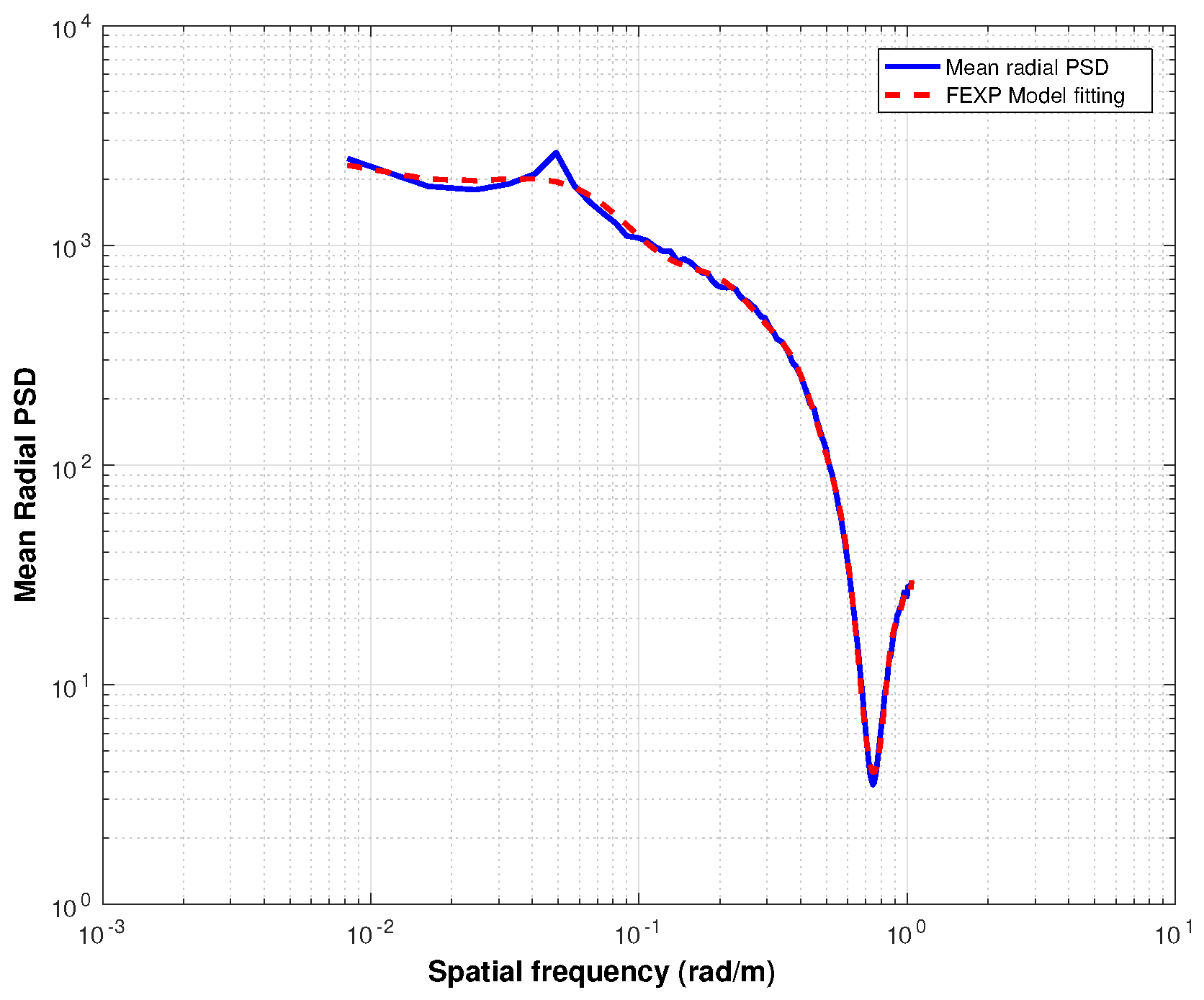
2. Sea Surface Model

In this section, a model of the different features the sea can exhibit is shown. The model, as shown here, can be described by a reduced set of parameters that behave differently if they belong to low-wind sea, sea with medium-high waves or sea with an oil spill. To make the correct estimation of the different features, all must be present in the image because the algorithm works by comparison. Many natural surfaces in high-resolution SAR images exhibit long-term dependence behavior and scale-limited fractal properties. Specifically, the Long-Range Dependence (LRD) and Short-Range Dependence (SRD) properties describe respectively the high and low order correlation structure of a process. The generalized model of the sea SAR Power Spectral Density (PSD) is in the form:

$$E\left[S\left(k\right)\right]\propto k^{-\delta }$$

(1)

where k is the wavenumber, δ is a real number and $E[·]$ is the expectation operator. It means that the PSD, as a function of the wave number, is approximately a straight line with a negative slope in a log-log scale. The Fractional Exponential (FEXP) models preserve the negative slope of the long-memory data of the PSD near the origin. Through the so-called SRD functions, the shape and the slope of the PSD can be modeled. The spectral model, as described in [9], is:

$$S_{FEXP}\left(k\right)=|2sin\left(\frac{k}{2}\right){|}^{-2d}exp\left\{\sum _{l=0}^q{\eta }_l{z}_l\left(k\right)\right\}$$

(2)

where q is the polynomial order, d (namely fractional differencing parameter, with $0\le d<1.5$) and ${\eta }_l$ are the real parameters of the model to be estimated. The class of FEXP model used here is the polynomial FEXP model, where $z_l\left(k\right)=k^l$. Here, we used $q=15$. In (2), the first term is the LRD function, and the second one is the SRD function. By using a linear regression with the estimated radial PSD in a log-log scale, the d parameter can be estimated ( $\widehat{d}$, which depends on the SAR image roughness). Then, by inverting the model, an estimate of the SRD component can be determined. By using a fractal spectral characterization of the sea surface PSD [9], in particular the FEXP model, it is possible to reject look-alikes. In order to discriminate oil spills from lack of wind in sea SAR imagery, only two parameters are needed, $\widehat{d}$ and the mean value of the SRD component ${\overline{A}}_{SRD}$, which depends on the amplitude of the backscattered signal (see [9] for the reference). That mean value can be expressed as the mean value of the radial PSD of the SRD part, averaged over all possible wavenumbers k. The criterion of classification is shown in (3):

$$\left\{\begin{array}{c}{\widehat{d}}_{CleanSea}\lesssim {\widehat{d}}_{Oil}<{\widehat{d}}_{LowWind}\hfill \\ {\overline{A}}_{CleanSea}>{\overline{A}}_{Oil}\hfill \\ {\overline{A}}_{CleanSea}\gg {\overline{A}}_{LowWind}\hfill \end{array}\right.$$

(3)

Figure 2 shows the fitting (in the dashed line) of the FEXP model with the mean radial PSD, showing an excellent level of agreement.

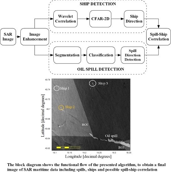
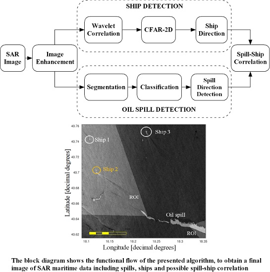
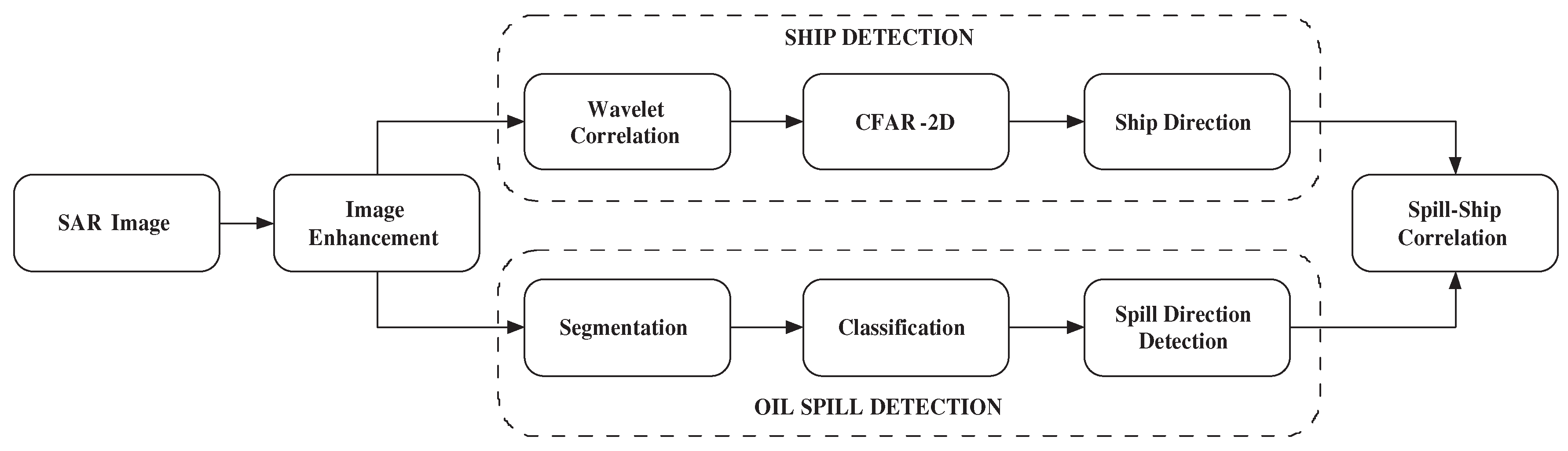
3. Oil Spill and Ship Detection Algorithms

3.1. Image Enhancement

A SAR image is generated by transmitting a coherent electromagnetic wave and subsequently processing the backscattered signal from the illuminated scene. However, due to the interference processes between scatterers, speckle noise is introduced into the image.

Therefore, it is important to apply suitable speckle reduction methods prior to carrying out any image processing. Such methods are able to smooth speckle noise, while retaining as much detailed information as possible.

Based on the studies in [10], the gamma-Maximum-A-Posteriori (MAP) filter with a $3\times 3$ kernel size has been chosen since it is a good trade-off between the noise reduction and the preservation of details.

The following step is the contrast enhancement, involving morphological operators as shown in (4):

$$I{m}_{out}=(I{m}_{in}•B)\ominus B$$

(4)

where $I{m}_{in}$ is the image to be processed, B is the structuring element, • is the closing operator and ⊖ is the erosion operator [11]. We used as the structuring element a square with a side of five pixels. The structuring element is not part of the image; it is only a shape element whose only purpose is to define how the morphological operators work. The image is then filtered to reduce residual noise with a $5\times 5$ Gaussian filter.

Figure 3 shows a CSK StripMap HIMAGE image from data acquired on 22 August 2009 (Adriatic Sea) with HH polarization by COSMO-2 satellite, before image enhancement processing. A pair of slicks is visible, with the leftmost slick probably having undergone a process of drift due to surface current. Figure 4 shows the result of the morphological processing, which reduces the granularity of the images, enhancing details like waves without compromising the sharpness of the slick borders (that means, preserving the high frequency components of the image).

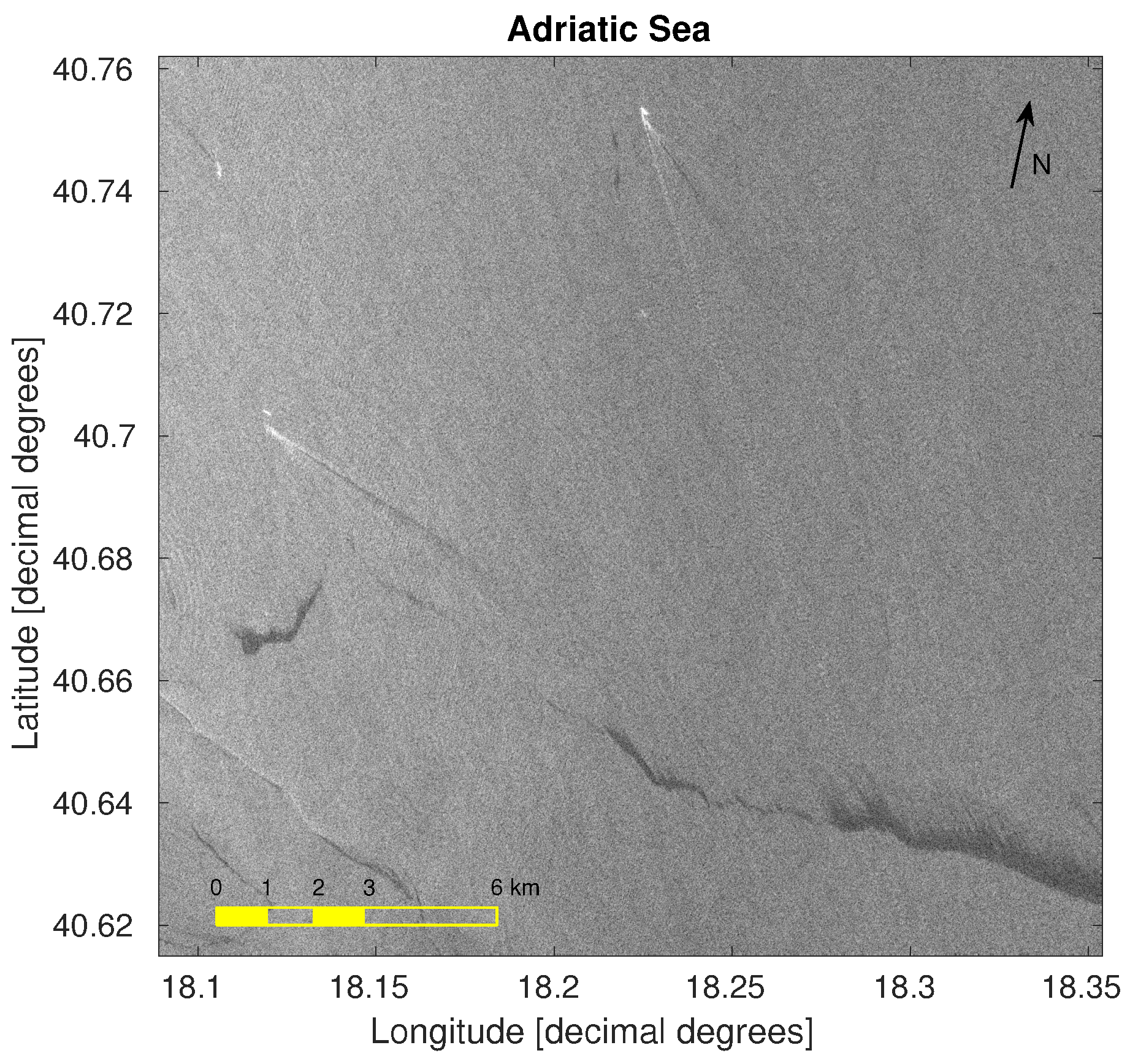
3.2. Oil Spill Detection

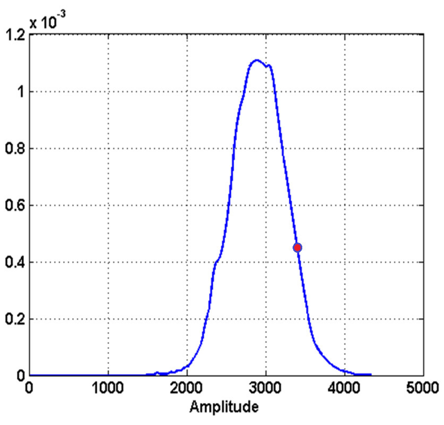
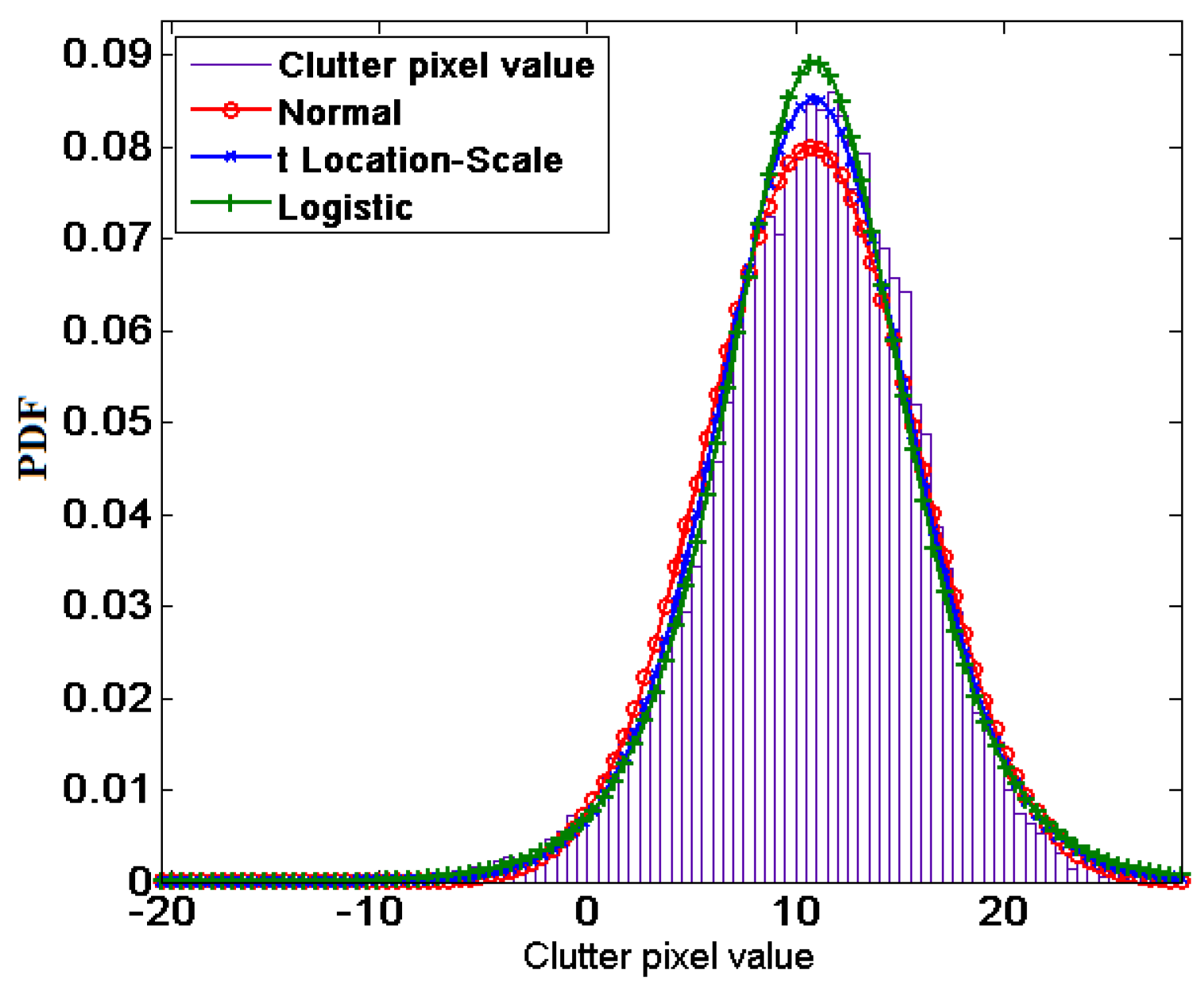
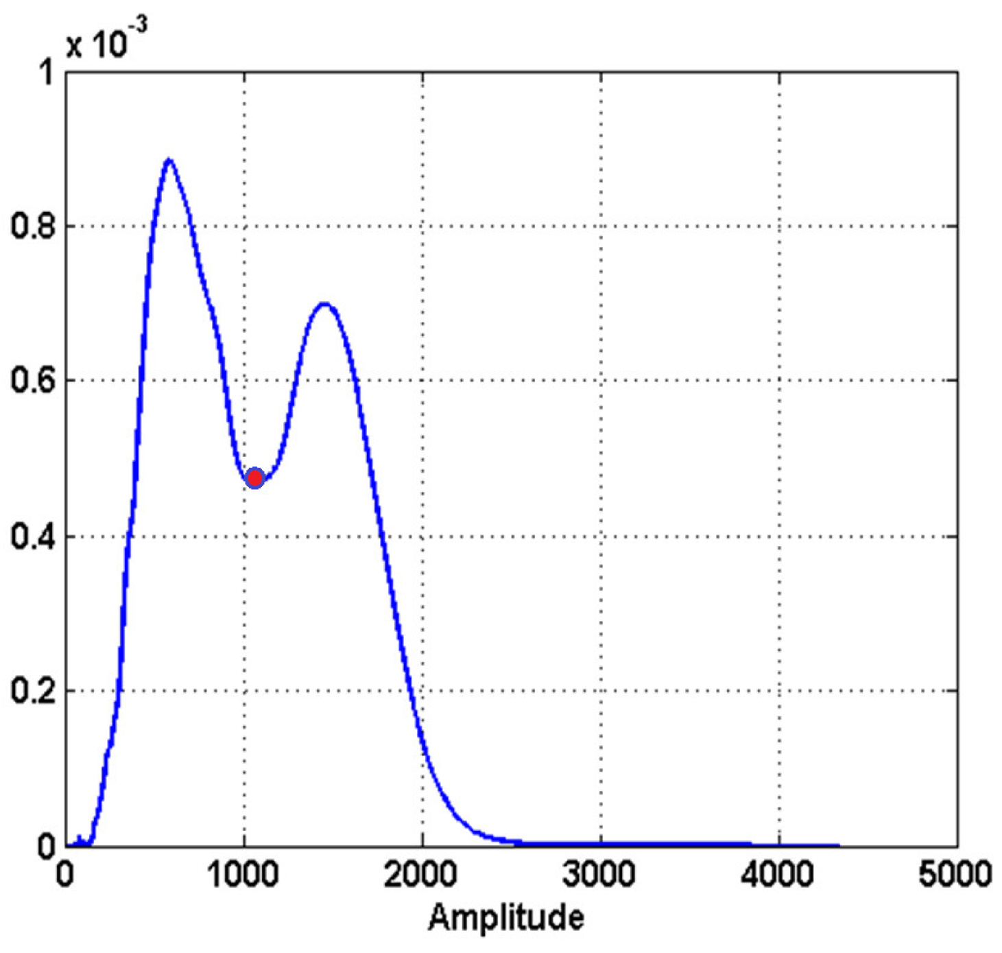
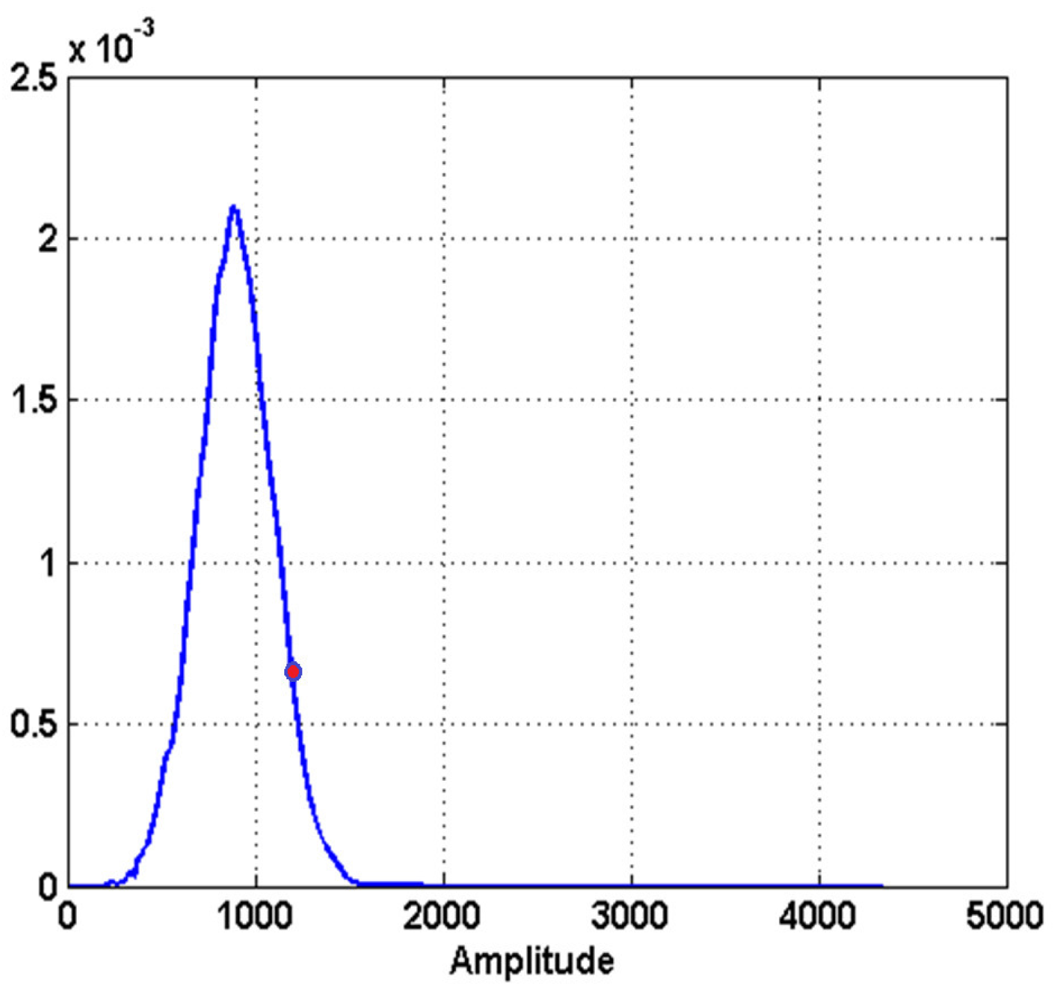
3.2.1. Image Segmentation

The first operation is the segmentation of the image to automatically detect the areas with the lowest gray level, which may be associated with oil spills or look-alikes. In fact, the intensity of the sea backscatter signal is mainly due to the short gravity and capillary waves (1- to 100-cm wavelength), according to Bragg scattering theory. An oil film on the sea surface damps these kinds of waves, consequently reducing the measured backscattering. However, careful image analysis is required because low backscattering areas might also be caused by natural phenomena, e.g., wind falls. The segmentation algorithm involves the estimation of the histograms of the image divided into blocks using the Kernel Density Estimation (KDE) method [12], a non-parametric way for estimating the Probability Density Function (PDF) of a random variable. Let $[x_1,x_2,\dots ,x_n]$ be independent and identically distributed samples drawn from some distribution with an unknown density f. Its kernel density estimator is given by (5):

$${\tilde{f}}_h\left(p\right)=\frac{1}{nh}\sum _{i=1}^{n}K\left(\frac{p-p_i}{h}\right)$$

(5)

where $K(·)$ is the kernel function (in this application, it is Gaussian) and h>0 is a smoothing parameter. Ideally, h should be as small as possible, but choosing low values of h makes the variance of the estimator too high. On the other hand, a large bandwidth cannot resolve a multimodal distribution. For the pixels to be considered as oil spills, a threshold $Th$ can be chosen adaptively by analyzing the histograms of the data, which can be of three types: low reflectivity zone, bimodal with low reflectivity area and sea or sea only. Values lower than $Th$ are selected as potential oil-spill candidates. The steps of the threshold searching algorithm are here listed:

• Step 1: search the smaller among all of the maxima of the PDF of the data in the block under observation ($M_{min}$);
• Step 2: estimate the derivative of the PDF to find possible saddle points;
• Step 3: sort in ascending order the value of saddle points and keep as a candidate threshold $Th$ the smaller one;
• Step 4: if no saddle points are found, select as a $Th$ candidate the point that is distant by one standard deviation toward the right from the maximum of the PDF;
• Step 5: memorize the $Th$ candidate and repeat for every block;
• Step 6: sort all of the $Th$ candidates in ascending order;
• Step 7: choose as a threshold $Th$ the first candidate in ascending order whose amplitude is greater than $M_{min}$.

Examples of $Th$ candidates are shown with a red dot from Figure 5, Figure 6 to Figure 7. The red dots represent the position on the distribution of the maximum possible value accepted belonging to an oil slick area. A this point of the processing, they can also belong to wind falls or algae patches.

The results of the segmentation algorithm provide a binary mask that can be applied on the enhanced image to separate pixels belonging to potential candidates from rejections. Figure 8 shows the results of the segmentation algorithm on the previously presented image. By visual inspection only, two potential candidates appear. Especially, the patch in the lower right of the image shows the typical behavior of drifting due to sea currents. Heuristic considerations based on the behavior of look-alikes suggest that in this image, no visible zones of algae patches or low wind zones are present. However, in future refinements of this study, ancillary data regarding wind fields and chlorophyll content could be provided to further sustain these observations.

A more complex image was selected to demonstrate the need of a classification procedure after the segmentation algorithm. The image in Figure 9, acquired from another CSK StripMap HIMAGE data on 13 May 2008 (Ionian Sea) at HH polarization by the COSMO-1 satellite, shows the results of the enhancement processing, where some low wind zones are present, while Figure 10 shows the results of the segmentation. Two zones with false alarms are evident in the corner, by making simple shape assumptions.

3.2.2. Classification

As stated before, for a correct detection of an oil spill with respect to a false alarm, a classification procedure that works on the segmented image is needed. To do this, we need to estimate the fractional differencing parameter $\widehat{d}$ and the mean value of the SRD component ${\overline{A}}_{SRD}$. This procedure is performed over the ensemble of the pixels that compose the various dark zones that were detected by the segmentation algorithm. After the estimation of the parameters, the criterion shown in (3) can be applied. The results obtained for the two images are here listed in

Table 1. Classification parameters for Adriatic Sea dataset.

	$\widehat{\mathit{d}}$	${\overline{\mathit{A}}}_{\mathbf{SRD}}$
Clean sea	0.1206	216.2745
Oil spill	0.1580	100.4706

for the Adriatic Sea dataset and in

Table 2. Classification parameters for Ionian Sea dataset.

	$\widehat{\mathit{d}}$	${\overline{\mathit{A}}}_{\mathbf{SRD}}$
Clean sea	0.3737	49.1312
Oil spill	0.5666	12.8820
Wind fall	1.2004	1.4208

for the Ionian Sea dataset.

As one can easily observe, the results shown in the tables are completely in accordance with the rule shown in (3).

Figure 11 and Figure 12 show the results of the oil spill classification algorithm applied on the segmented images.

3.2.3. Oil Spill Direction Estimation

Once an oil spill has been recognized, its direction estimation is performed by means of the Discrete Radon Transform (DRT). This is applied to the binary image resulting from the classification algorithm (See Figure 11 and Figure 12). In fact, owing to its energy concentration capability, thin segments give rise to narrow peaks in the Radon space (RS) ($\rho -\theta$); the coordinates of the local maximum (${\rho }_0-{\theta }_0$) are the polar parameters of the straight line along which the segment lies. This property can be advantageously exploited for estimating the detection of segments [13]. At this point, the binary image of an oil spill would be composed by one or more patches. Since the oil spills are generated by moving ships, such patches usually have a linear behavior and a specific direction. It is understood that discharges from ships that have different dynamics (e.g., ships that discharge and then move on) may be possible, but this situation is not investigated in this article. Nevertheless, these slicks would not have an elongated and thin appearance, but rather a quite spread appearance, making the possibility of finding relevant peaks in the DRT quite difficult. First, some spatial parameters of each dark patch are calculated, such as centroid, orientation and extreme points. Then, the greatest dark patch is chosen, and the distances between its centroid and its extremes are calculated. That particular patch is selected because it gives a greater contribution for the DRT, and only that one could be enough to get the region estimate where to search for a possible responsible ship.

3.3. Ship Detection

The proposed ship detection algorithm involves a novel approach, based on the analysis of SAR images by means of the joint use of the two-dimensional Discrete Wavelet Transform (2D-DWT) and 2D-CFAR [14].

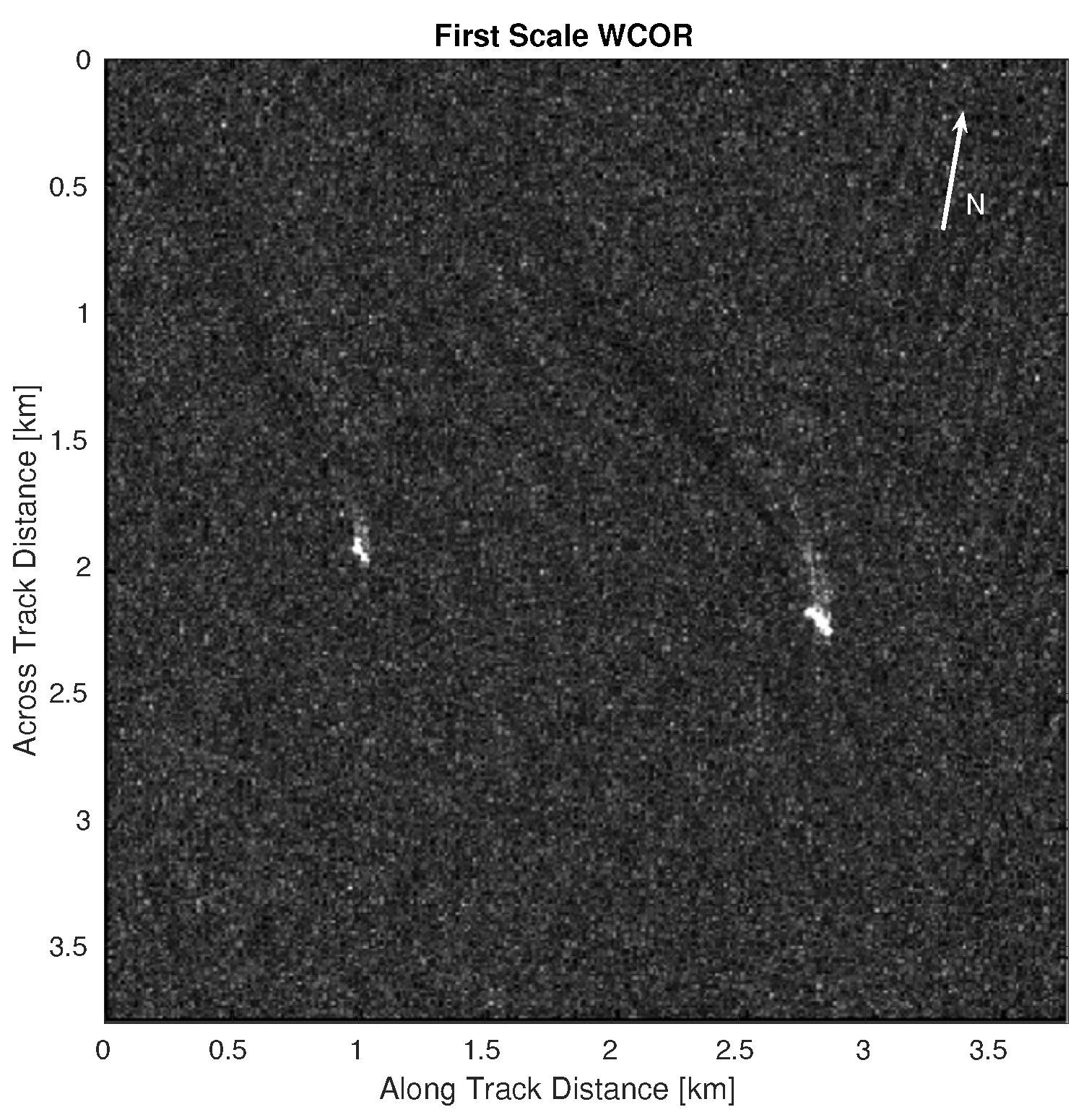
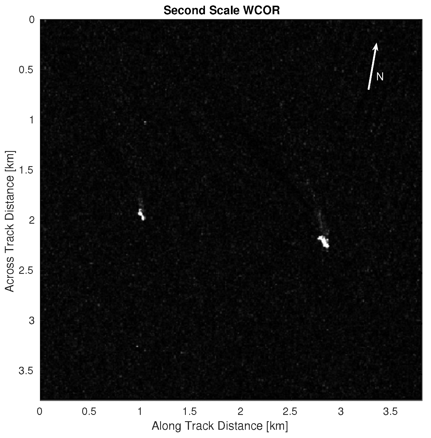
3.3.1. SAR Image Preprocessing (Wavelet Correlator)

In high resolution SAR images, it can be observed that a vessel behaves with a deterministic pattern. This fact explains why the presence of a ship is usually noticeable in the sub-bands (or scales) obtained when applying 2D-DWT. The two different scales and detail levels are shown in Figure 13 and Figure 14. This kind of discontinuity can even be transmitted over scales. On the contrary, orthogonality between the different wavelet subspaces ensures a quasi-decorrelation of the residual noise, behaving as a random distributed variable, identically distributed within each scale. These considerations lead to the Wavelet Correlator (WCOR) algorithm, which consists of calculating the modulus of the detailed images resulting from each scale [15]. This method takes advantage of the wavelet theory in order to suppress the noise and magnify the edge structures belonging to targets.

3.3.2. S-Detector

The first step, used as pre-screening processing, is based on a contrast parameter, namely significance [16,17]. The Significance (S-parameter) is defined as follows:

$$S=\frac{max\left\{\right|I_{WCOR}\left|\right\}-\mu }{\sigma }$$

(6)

where $I_{WCOR}$ represents the SAR image after the WCOR processing, μ is the mean value and σ is the standard deviation. First of all, the whole SAR image is divided into blocks. This allows for parallel computing to be implemented and therefore processing time to be sped up. Once all of the blocks are collected, the S-parameter is calculated for each block. The S-parameter will be large in the presence of a target due to the high backscattering level. In fact, the low number of target pixels in the block under test does not affect the mean value and the standard deviation, but there will be a strong peak value. On the other hand, if targets are not present, S will assume a low value due to the clutter level that has been reduced and smoothed by the WCOR processing. The blocks where S exceeds the detection threshold are considered to be candidates for containing targets, and they will be processed by the Wavelet CFAR (W-CFAR) in the second stage. The detection decision is made by comparing the value of the significance of the block under test against the detection threshold, which is calculated by means of the estimated Generalized Extreme Value (GEV) parameters and the desired probability of false alarm. The threshold Λ can be expressed as:

$$\Lambda =\left\{\begin{array}{cc}\alpha -\frac{\beta }{\zeta }[1-log\left(\frac{1}{1-P_{FA}^S}\right)]\hfill & \mathrm{for}\zeta \ne 0\hfill \\ \alpha -\beta log\left[log\right(\frac{1}{1-P_{FA}^S}\left)\right]\hfill & \mathrm{for}\zeta =0\hfill \end{array}\right.$$

(7)

where α and β are the location and scale parameters representing the unknown normalization constants that are estimated from the clutter, ζ is the GEV distribution parameter and $P_{FA}^S$ the false alarm rate.

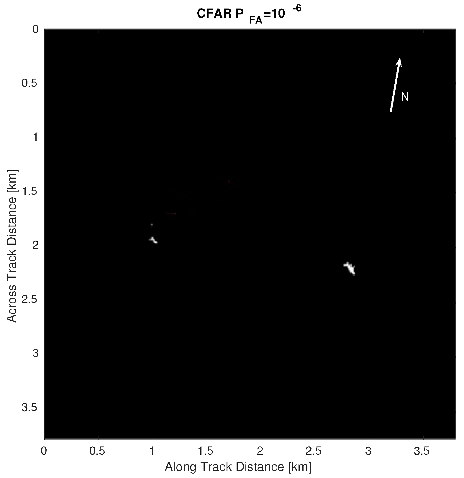
3.3.3. W-CFAR

After the pre-screening processing, all of the blocks whose S value exceeds the threshold are processed by the W-CFAR detector [18]. After the WCOR algorithm has been applied to the SAR image, the sea clutter is perfectly fitted by the log normal distribution. Furthermore, if a log-amplifier is applied to each pixel of the image, the result is a clutter Gaussian trend of the background (see Figure 15). As a reference, also two different fitting are included, the logistic distribution in green and the t-location scale distribution in blue, both overestimating the mean value of the real distribution.

The detector proposed by Goldstein in [19] is the so-called log-T detector. Under the hypothesis that clutter has a log normal distribution, it can be demonstrated that the optimal detector in the case of log normal clutter can be written in the form:

$$\underset{{\xi }_0}{\underbrace{log\left(V_0\right)}}\ge \underset{T^{\prime }}{\underbrace{{\sigma }_{c}T+log\left({\mu }_c\right)}}\Rightarrow {\xi }_0\ge T^{\prime }$$

(8)

where $V_0$ is the clutter value in the cell, ${\sigma }_c$ and ${\mu }_c$ are the parameters of the log normal distribution and $T\prime$ is the threshold for which the desired probability of false alarm ($P_{FA}$) is equal to:

$$P_{FA}={\int }_{T^{\prime }}^{\infty }{p}_c\left(t\right)dt$$

(9)

where $p_c\left(t\right)$ is the PDF of the test statistic ${\xi }_0$, which is normally distributed with standard deviation ${\sigma }_c$ and mean ${\mu }_c$. Figure 13 shows the application of the first-scale WCOR processing. Figure 14 shows instead the pre-detection results after the application of the S-detector after a second-scale WCOR processing. The result of the W-CFAR in the last step of the detection algorithm is shown in Figure 16.

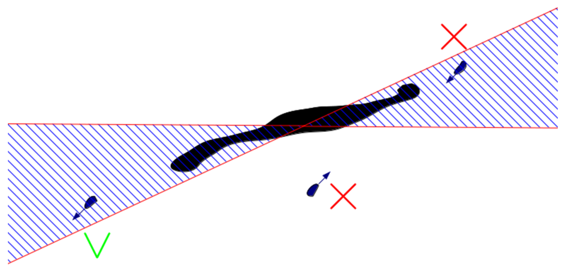
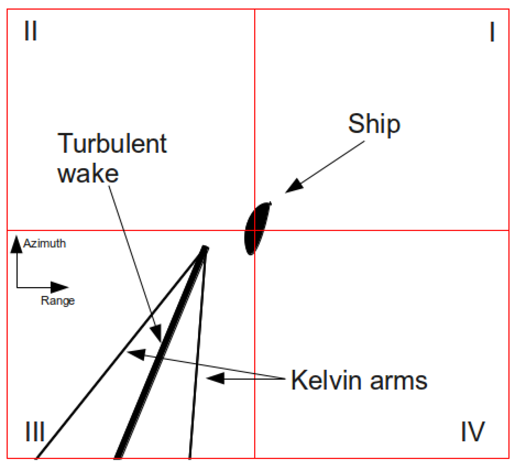
3.4. Ship’s Direction Estimation

To extract the ship’s complete features, a heading estimation is necessary. The ship’s direction is provided by means of the DRT applied on the binary image returned by the ship detection algorithm, on a window (wide enough to include the ship’s wake) centered in the ship’s centroid. Unfortunately, the DRT is ambiguous of ${180}^{\circ }$. Assuming the ship’s direction is the same as the wake, the ambiguity problem has been fixed by the following steps:

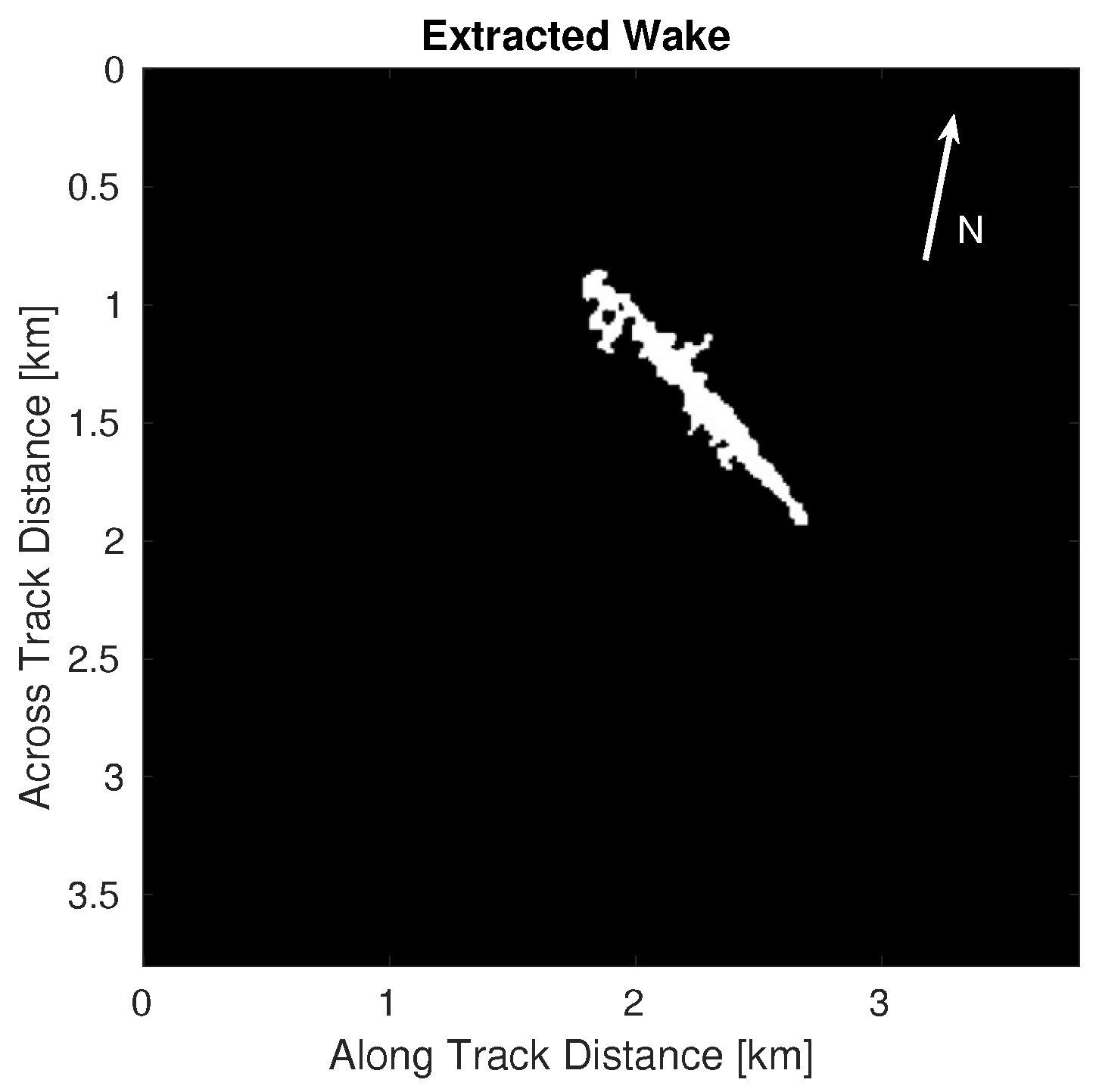
• wake extraction (performed by means of segmentation algorithm with different parameters);
• DRT over four quarters of the window.

The quarter containing the most wake arms is identified by the maximum of the RT among all of the quarters. Actually only two of the four quarters are examined since the ship’s direction is known and the DRT is applied only on an angular sector of ${30}^{\circ }$ of the two quarters under test. This removes the ambiguity and allows one to define the quarter of origin and thus its direction. Figure 17 shows the layout for ship direction determination.

The first step in the automatic wake detection algorithm consists of the ship detection that is described in Section 3.3.1 and Section 3.3.2. Then, the connected components labeling was applied to the binary image obtained by the previous algorithm to calculate the center of mass (centroid) of every ship as an isolated area of bright pixels linked to each other. This operation is performed for the proper elimination of the pixels belonging to the ships by replacing them with the mean values of the image amplitude. This is necessary as the areas corresponding to the ships are so bright that they would prevent the detection of any wake or linear structure. After all of ships are properly located and replaced by the mean value, windows of 1000 × 1000 pixels centered around the ship’s location were transformed into the Radon space. The size of the window that is extracted from the whole image is quite important as the Radon transform will be most efficient when such an extent is about the size of the wake. The greater the window in comparison with the wake, the lower its signal-to-noise ratio. As most of the encountered wakes did not exceed several hundred pixels, so this size proved to be optimal. It is worth pointing out that in an SAR image, the ship wake can be treated as a look-alike because of its darker appearance. Therefore, prior to performing the Radon transform, the algorithm described in Section 3.2.1 has been applied. That algorithm can be applied because the wake appears as a dark area with respect to the pixel representing the sea in the image crop. In this step, we assume that the slick is not very close to the ship; otherwise, some difficulties may arise in automatically differentiating slicks from wakes if they are in the same image crop around the ship. In this way, the noise effect is reduced since this algorithm gives a binary image of the wake. If some isolated pixels are returned, during the integration process, they do not provide a maximum point in the Radon space if a linear structure originated by the wake is present. This algorithm is based on the edge detection by means of Prewitt’s gradient [20]. Then, a morphological processing is applied and, after that, a Gaussian filtering to transform from a binary image to a gray level image. Finally, a thresholding operation returns the binary image. The idea of automatic wake detection is based on searching the maximum value in the Radon space. This procedure assumes that every maximum corresponds to a different line structure in the image. With the Radon coordinates, an estimate of the angular direction is provided. Figure 18 shows the results of the wake extraction algorithm applied on the wake of ship on the right in Figure 13.

3.5. Correlation between Oil Spill and Ship

In this final processing step, the detected ships are correlated with oil slick behavior in order to extract some data belonging only to those ships involved in illegal acts. First of all, by exploiting the linearity of the oil spill, an angular sector (Region Of Interest (ROI)) around the centroid of about ${60}^{\circ }$ is derived. Thus, all of the ships in the ROI that head away from the oil spill are likely to be the responsible candidates. All of the other ships are rejected. The derivation of this angle is based mostly on considerations on the ship dynamics after dumping. Usually, ships dump the oil while continuing through a straight route, while more distant from the spill, they can change the route, but usually not with extreme deviation from a straight line. Moreover, a guard angular sector is included in the aperture. An example of the procedure is shown in Figure 19.

Therefore, two constraints must be satisfied in order to consider a ship as potentially responsible:

• the ship must belong to the angular sector;
• the ship’s position and direction must be consistent with the oil spill position and direction.

Once all of the candidate ships are detected, some of their features are extracted: area, length, width and distance to the oil spill extreme.

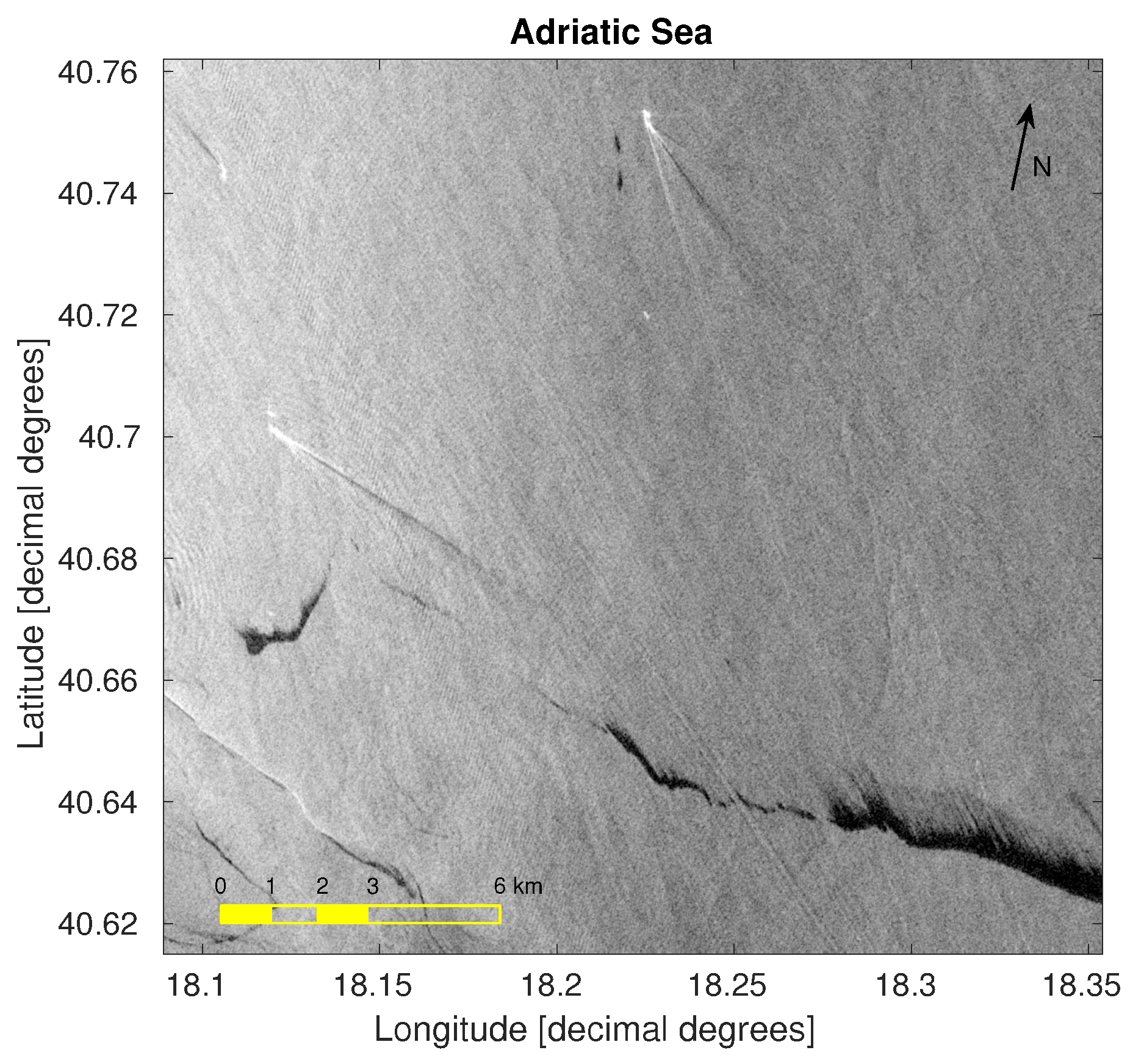
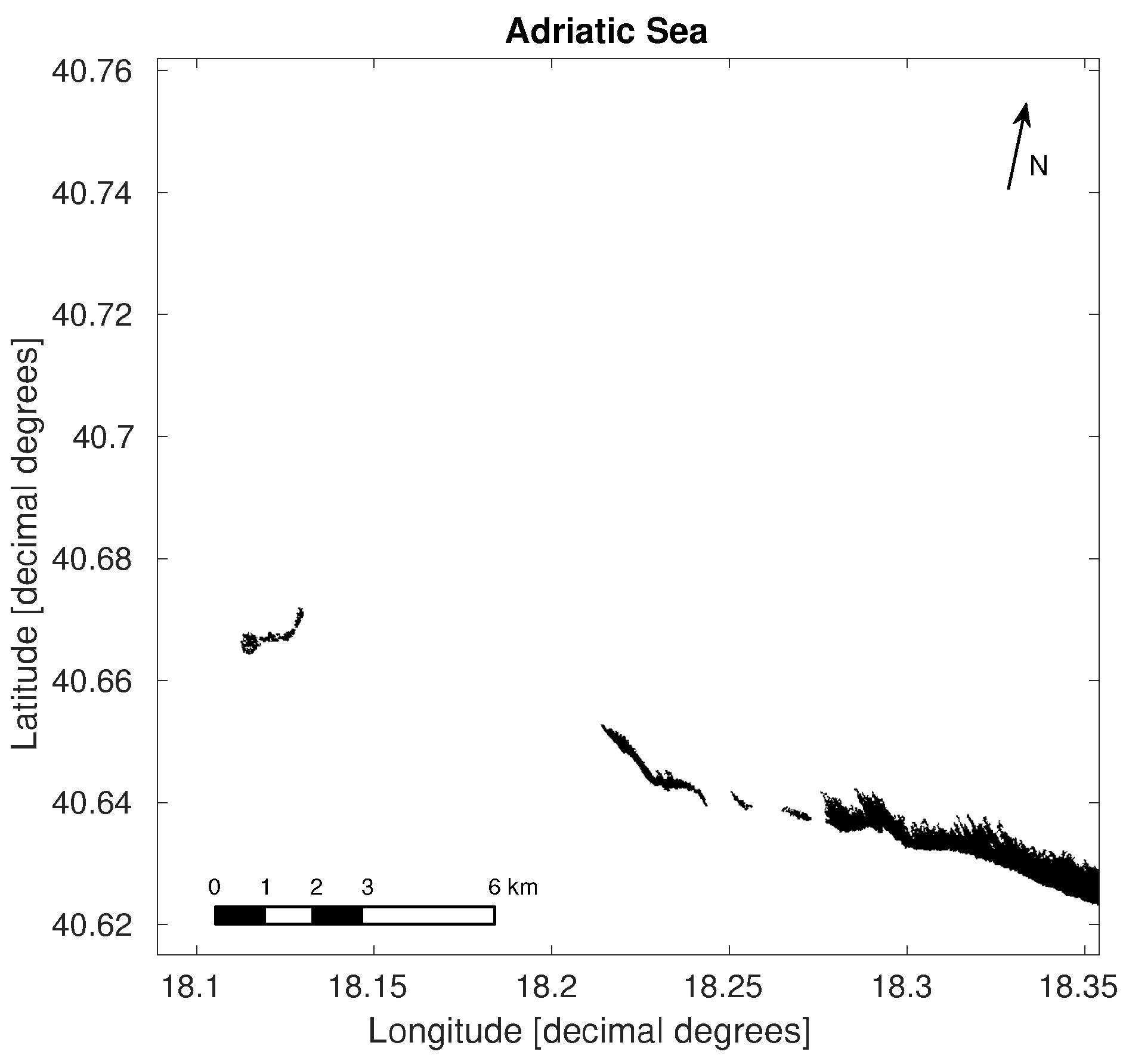
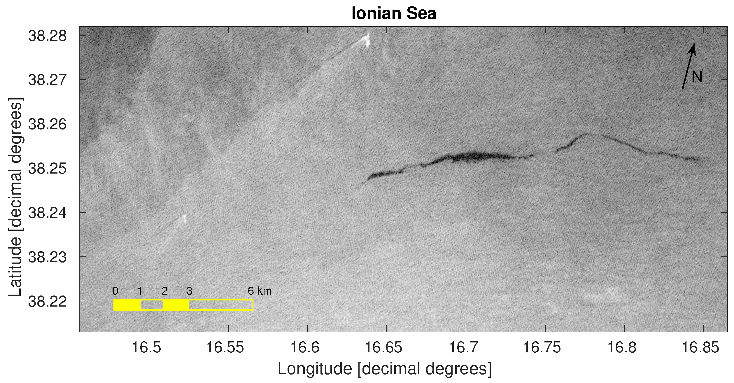
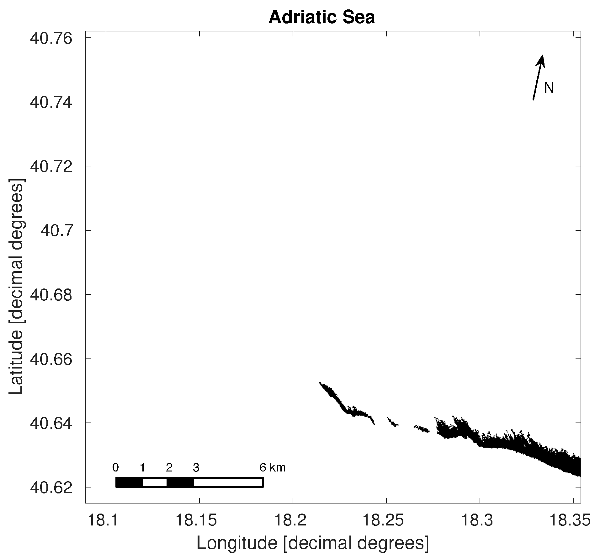
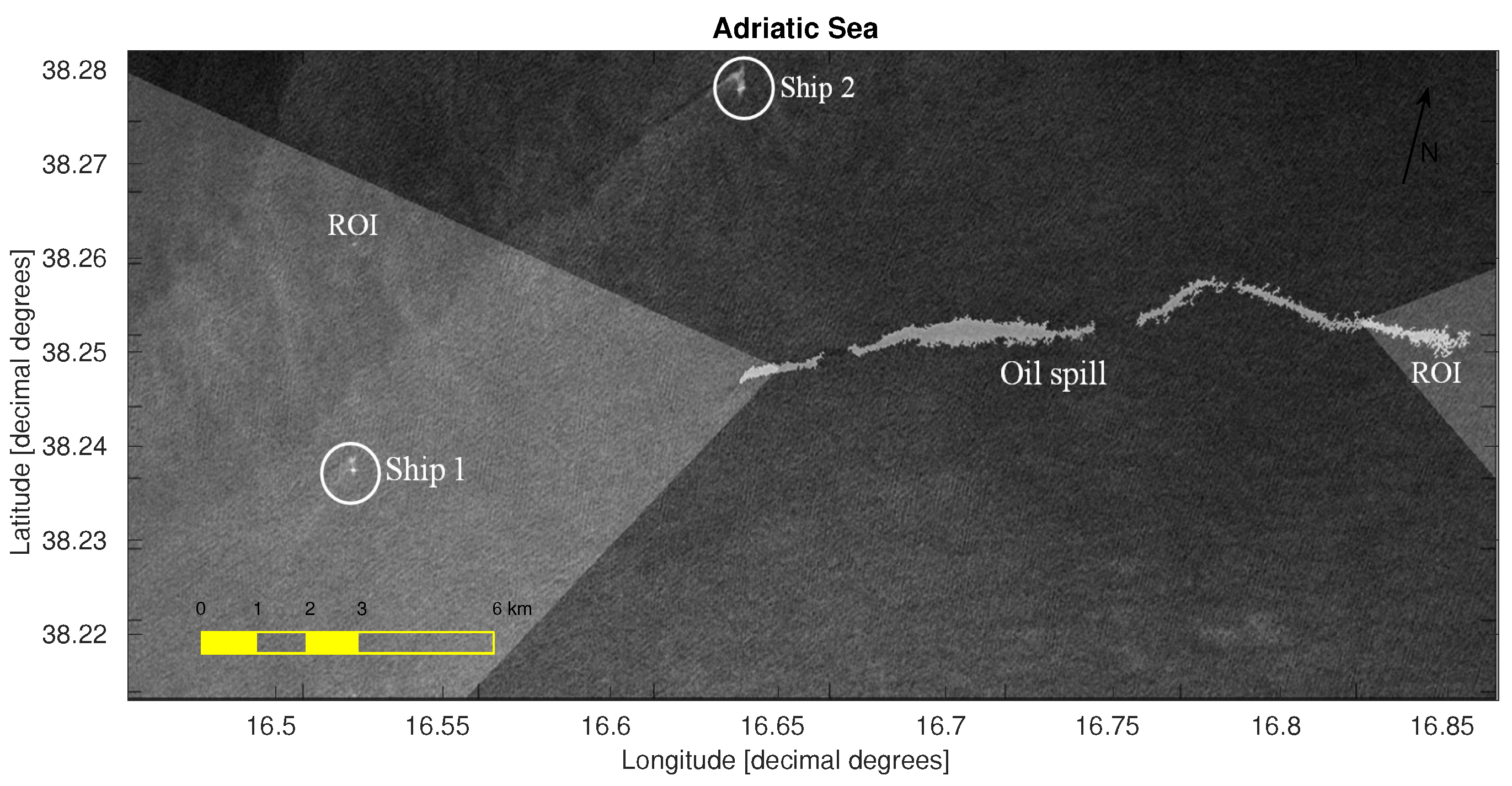
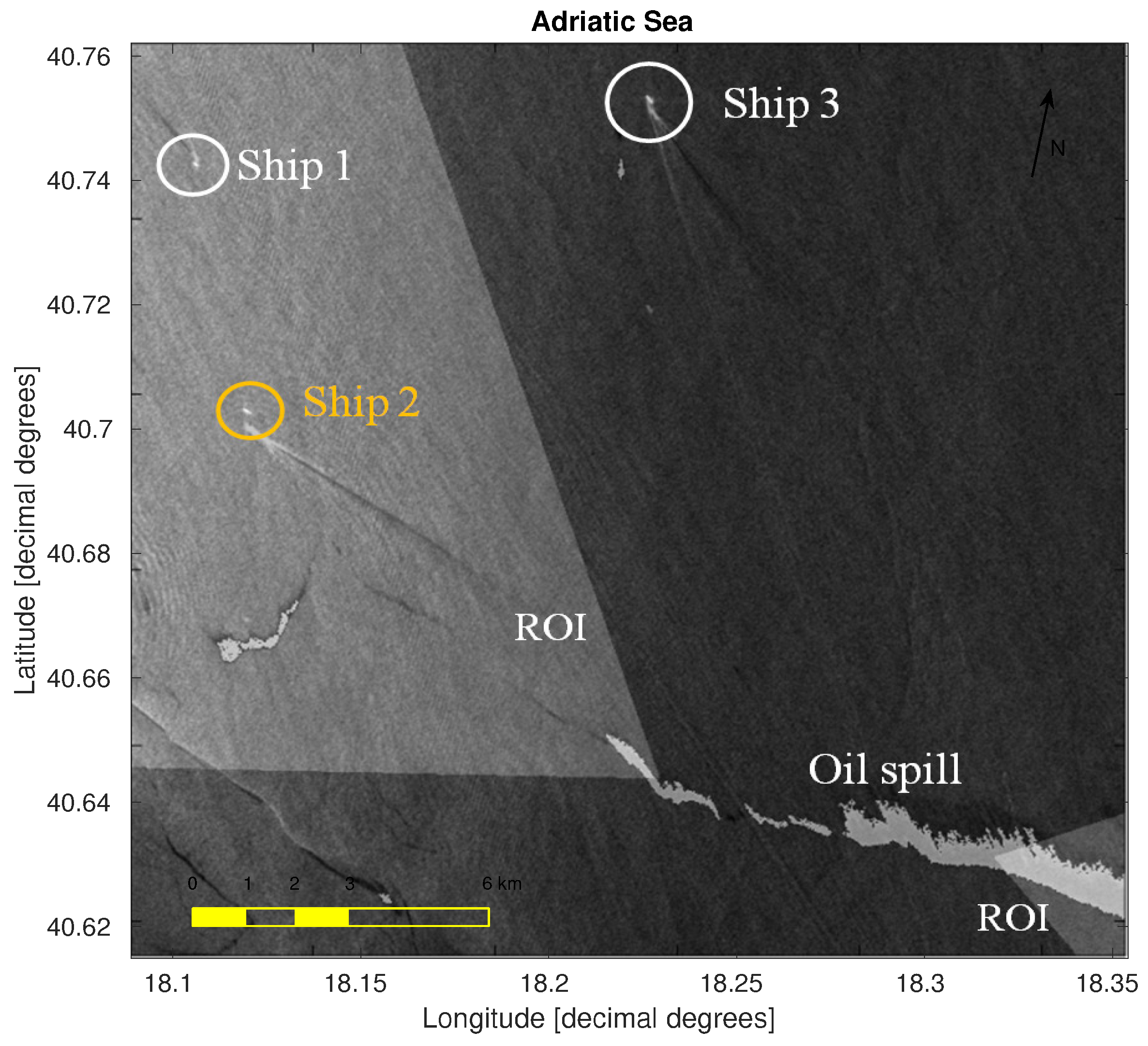
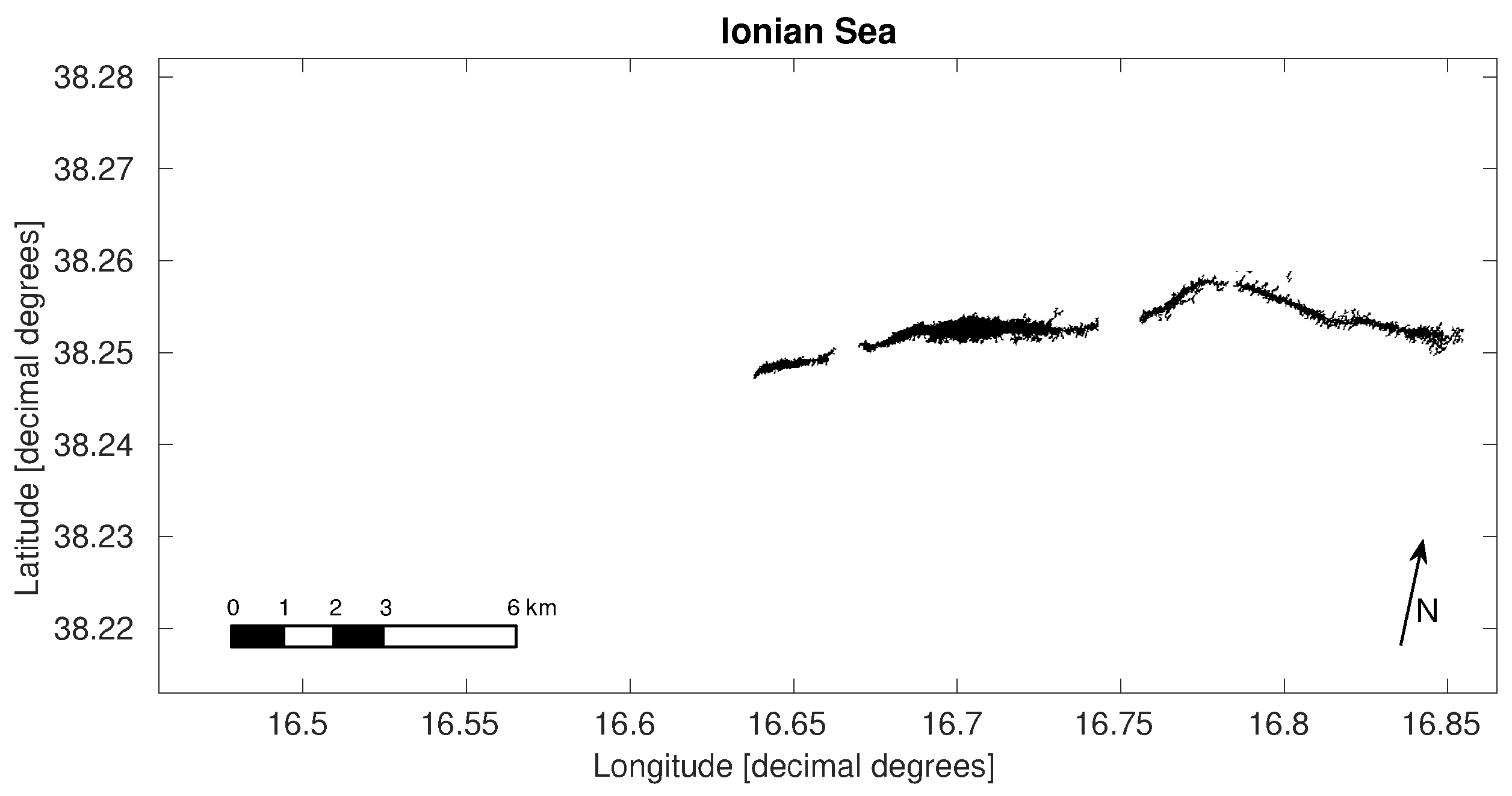
4. Ship-Spill Correlation Results

In this final section, we show the results obtained from processing two CSK images. As already stated, they represent sea surface covered by oil spills (classified as such by the classification algorithm) and various ships. Their azimuth and range spatial resolution is 2.5 m. Unfortunately, we could not find datasets that contain evident algae patches and oil spills. For this reason, the discussion on the results in this paper is limited to the separation between sea, oil spill and low wind zones. Further analysis can be made with the same proposed method, when proper imagery is found. Figure 20 shows the results for the Ionian Sea dataset. Despite the presence of a huge oil slick and two ships detected, the algorithm does not recognize these ships as being possible candidates; Ship 2 does not belong to the ROI, while Ship 1 has no wake, so it is not possible to relate the spill to the ship. Nevertheless, the algorithm correctly detects low wind zones, spill and ships. On the contrary, as we can see in Figure 21 for the Adriatic Sea dataset, only Ship 2 satisfies the conditions of being considered potentially responsible, since Ship 3 is outside the ROI and Ship 1 heads towards the spill. It should be noted, however, that the candidate ship may have simply crossed the slick without causing it. There are many dynamics that can happen, so the ship can be flagged for a human operator to consider other data, if needed. Brighter zones correspond to the detected oil spill (output of classification algorithm) and ROI. In

Table 3. Features of the potential responsible ship.

Area	8870 m${}^2$
Length	228 m
Width	49.5 m
Distance from the oil spill extreme	11.23 km

, the spatial features of Ship 2 are shown.

Moreover, the use of the W-CFAR detector resulted in a drastic reduction in processing time. In the whole process, nearly the totality of the processing time would be occupied by the CFAR algorithm. It is worth mentioning that typically, a CFAR algorithm is applied directly to the entire image, therefore producing a very slow detection algorithm. In the case of the standard CFAR procedure, for an SAR image with order ${10}^8$ pixels, the processor needs 15 h of computation time, compared to 6 min and 7 min of processing time for the two images, respectively, for the whole image enhancement, segmentation and classification process. Instead, the use of the wavelet correlator brings down this time to the order of a few tens of minutes, at least. In our tests, the time of processing for the ship detection algorithm is cut down to an average of 16 min, balancing accordingly the time spent for the two branches of the algorithm. The elaboration was carried out on a Intel^TM Core i7 CPU 860 @ 2.80 GHz with eight cores using parallel processing.

5. Conclusions

In this work, we presented an algorithm that is able to detect oil spills and the candidate ship responsible for illegal dumping in the sea. Firstly, we applied a classification algorithm based on FEXP models that appear to correctly discriminate between oil spill and look-alikes. Then, we used the DRT for the detected slick to analyze its linear behavior, thus defining a possible angular sector in which a responsible ship and its wake can be searched. Finally, we developed a fast segmentation algorithm to work with large images even on commercial machines. CSK images appear also to be very suitable for the detection of ships, which are all highlighted even with very low $P_{FA}$ (${10}^{-6}$–${10}^{-8}$). This system can have some applications especially for early warning, illegal activity detection and pollution control. This is especially true in the Mediterranean Sea, characterized by heavy marine traffic. Regarding future developments, it is possible to include information from other sources like route tracking systems, AIS and national or international databases, to enhance system performances. More in detail, the proposed algorithm can be included in a system of support to decision, impacting directly the decisional processes that can bring operational decisions in maritime environment management.

References

- Galland, F.; Réfrégier, P.; Germain, O. Synthetic Aperture Radar oil spill segmentation by stochastic complexity minimization. Geosci. Remote Sens. Lett. 2004, 1, 295–299. [Google Scholar] [CrossRef]
- Oil Spill Detection Examples: Maersk Kiera. Available online: http://www.emsa.europa.eu/csn-menu/csn-service/oil-spill-detection-examples/item/1873-oil-spill-detection-examples-maersk-kiera-february-2012.html (accessed on 2 March 2017).
- Migliaccio, M.; Gambardella, A.; Tranfaglia, M. SAR Polarimetry to Observe Oil Spills. IEEE Trans. Geosci. Remote Sens. 2007, 45, 506–511. [Google Scholar] [CrossRef]
- Cloude, S.R.; Pottier, E. A review of target decomposition theorems in radar polarimetry. IEEE Trans. Geosci. Remote Sens. 1996, 34, 498–518. [Google Scholar] [CrossRef]
- Gambardella, A.; Migliaccio, M.; De Grandi, G. Wavelet polarimetric SAR signature analysis of sea oil spills and look-alike features. In Proceedings of the 2007 IEEE International Geoscience and Remote Sensing Symposium, Barcelona, Spain, 23–28 July 2007; pp. 983–986.
- Migliaccio, M.; Ferrara, G.; Gambardella, A.; Nunziata, F. A new stochastic model for oil spill observation by means of single-look SAR data. In Proceedings of the 2006 IEEE US/EU Baltic International Symposium, Klaipeda, Lithuania, 23–26 May 2006; pp. 1–6.
- Shirvany, R.; Chabert, M.; Tourneret, J.Y. Ship and Oil-Spill Detection Using the Degree of Polarization in Linear and Hybrid/Compact Dual-Pol SAR. IEEE J. Sel. Top. Appl. Earth Obs. Remote Sens. 2012, 5, 885–892. [Google Scholar] [CrossRef] [Green Version]
- Migliaccio, M.; Ferrara, G.; Gambardella, A.; Nunziata, F.; Sorrentino, A. A Physically Consistent Speckle Model for Marine SLC SAR Images. IEEE J. Ocean. Eng. 2007, 32, 839–847. [Google Scholar] [CrossRef]
- Bertacca, M.; Berizzi, F.; Dalle Mese, E. Long-Range Dependence Models for the Analysis and Discrimination of Sea-Surface in Sea SAR Imagery. In Image Processing for Remote Sensing, 1st ed.; Chen, C.H., Ed.; CRC Press: New York, NY, USA, 2007; pp. 189–223. [Google Scholar]
- Mansourpour, M.; Rajabi, M.A.; Blais, J.A.R. Effects and performance of speckle noise reduction filters on active radar and SAR images. In Proceedings of the 2006 International Society of Photogrammetry and Remote Sensing Symposium, Ankara, Turkey, 14–16 February 2006.
- Gonzalez, R.C.; Woods, R.E.; Eddins, S.L. Digital Image Processing Using MATLAB, 2nd ed.; Gatesmark Publishing: Knoxville, TN, USA, 2009. [Google Scholar]
- Epanechnikov, V. Non-Parametric Estimation of a Multivariate Probability Density. Theory Probab. Appl. 1969, 14, 153–158. [Google Scholar] [CrossRef]
- Lim, J.S. Two-Dimensional Signal and Image Processing, 15th ed.; Prentice Hall: Englewood Cliffs, NJ, USA, 1990; pp. 42–45. [Google Scholar]
- Staglianò, D.; Musetti, L.; Cataldo, D.; Baruzzi, A.; Martorella, M. Fast detection of maritime targets in high resolution SAR images. In Proceedings of the 2014 International Radar Conference, Lille, France, 13–17 October 2014.
- Staglianò, D.; Lupidi, A.; Berizzi, F. Ship detection from SAR images based on CFAR and wavelet transform. In Proceedings of the 2012 Tyrrhenian Workshop on Advances in Radar and Remote Sensing, Napoli, Italy, 12–14 September 2012; pp. 53–58.
- Tello, M.; Lopez-Martinez, C.; Mallorqui, J. A novel algorithm for ship detection in SAR imagery based on the Wavelet transform. Geosci. Remote Sens. Lett. 2005, 2, 201–205. [Google Scholar] [CrossRef]
- Tello, M.; Lopez-Martinez, C.; Mallorqui, J. Automatic vessel monitoring with single and multidimensional SAR images in the wavelet domain. ISPRS J. Photogramm. Remote Sens. 2006, 61, 260–278. [Google Scholar] [CrossRef]
- Pierre Haché, J. Probability of Detection for a GO-CFAR Radar Processor Using Envelope Detection Approximation. Master’s Thesis, Naval Postgraduate School, Monterey, CA, USA, September 1994. [Google Scholar]
- Goldstein, G. False alarm regulation in log normal and weibull clutter. IEEE Trans. Aerosp. Electron. Syst. 1973, 9, 260–278. [Google Scholar] [CrossRef]
- Prewitt, J.M.S. Object Enhancement and Extraction. In Picture processing and Psychopictorics, 1st ed.; Sacks Lipkin, B., Rosenfeld, A., Eds.; Academic Press: Orlando, FL, USA, 1970; pp. 75–149. [Google Scholar]