
Annual Gross Primary Production from Vegetation Indices: A Theoretically Sound Approach


Abstract
:
1. Introduction
2. A Theoretically Sound Approach
3. Materials and Methods
3.1. Study Area
3.2. Images
3.2.1. Daily PAR Images
3.2.2. Daily GPP Images
3.2.3. Daily VI Images
3.2.4. Vegetation Type Images
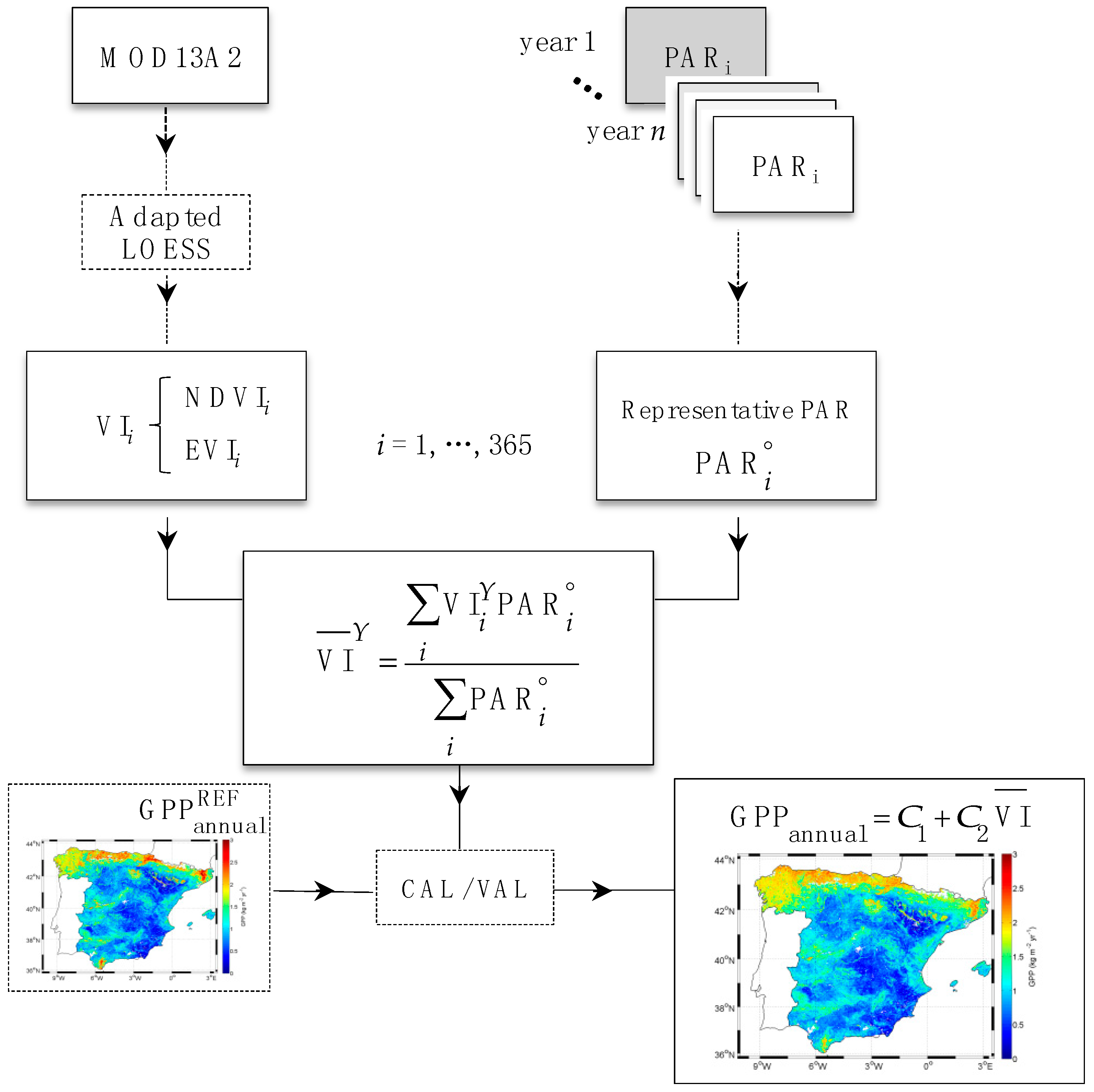
3.3. Methodology
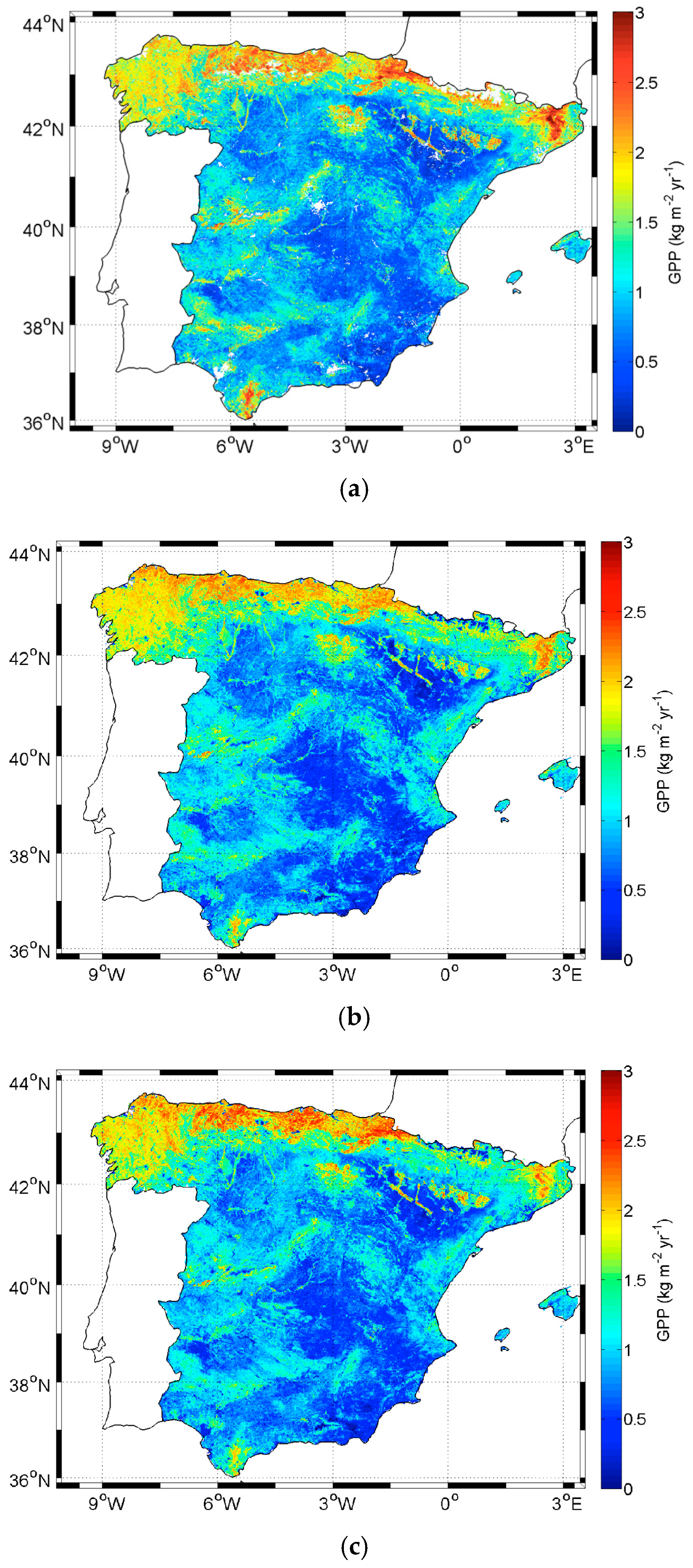
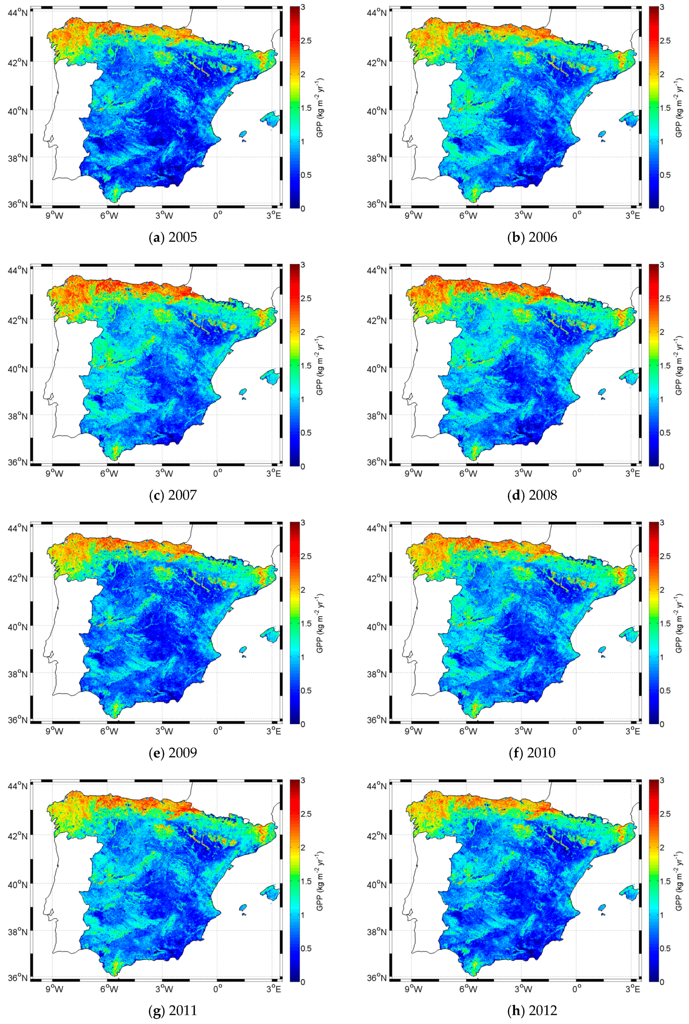
4. Results
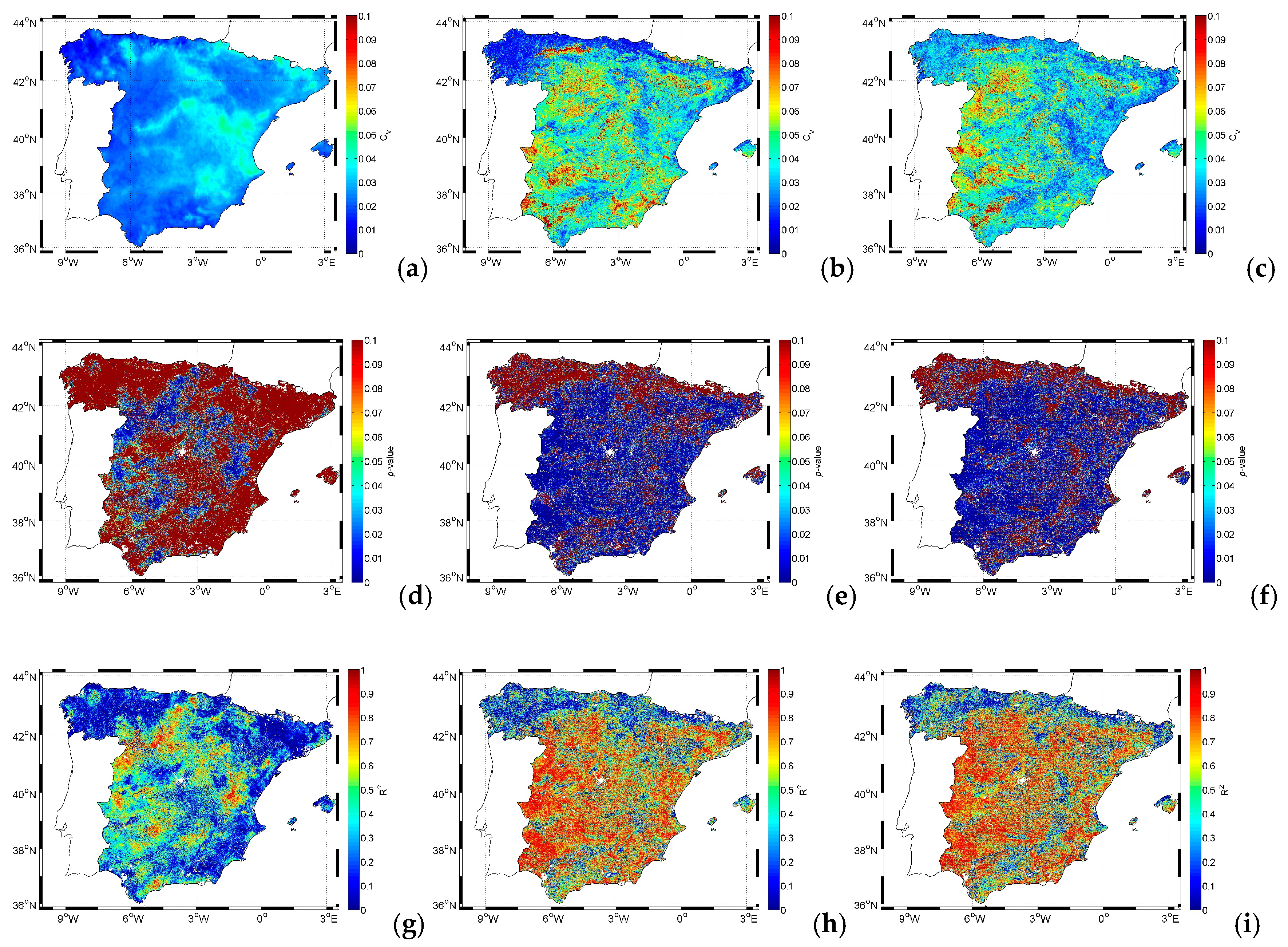
4.1. H1 Hypothesis Testing
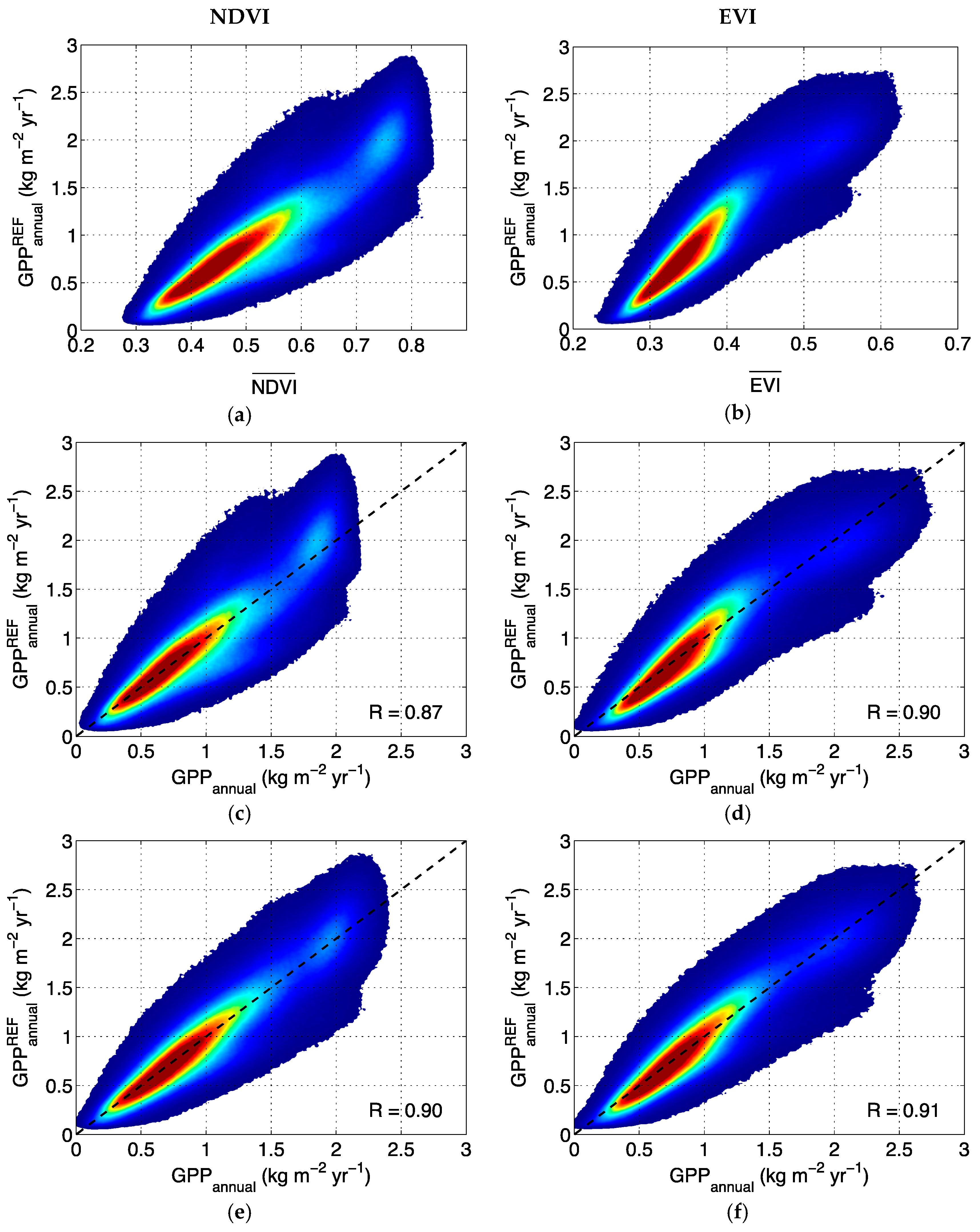
4.2. Calibration and Validation of the Semi-Empirical Model
5. Discussion
6. Conclusions
Acknowledgments
Author Contributions
Conflicts of Interest
References
- Reichtein, M.; Falge, E.; Baldocchi, D.; Papale, D.; Aubinet, M.; Berbigier, P.; Bernhofer, C.; Buchmann, N.; Gilmanov, T.; Granier, A.; et al. On the separation of net ecosystem exchange into assimilation and ecosystem respiration: Review and improved algorithm. Glob. Chang. Ecol. 2005, 11, 1424–1439. [Google Scholar] [CrossRef]
- Huete, A.; Ponce-Campos, G.; Zhang, Y.; Restrepo-Coupe, N.; Ma, X.; Moran, M.S. Monitoring photosynthesis from space. In Land Resources Monitoring, Modeling, and Mapping with Remote Sensing; Thenkabail, P.S., Ed.; CRC Press: Boca Raton, FL, USA, 2015; pp. 3–22. [Google Scholar]
- Mäkelä, A.; Kolari, P.; Karimäki, J.; Nikinmaa, E.; Perämäki, M.; Hari, P. Modelling five years of weather-driven variation of GPP in a boreal forest. Agric. For. Meteorol. 2006, 139, 382–398. [Google Scholar] [CrossRef]
- Gilabert, M.A.; Moreno, A.; Maselli, F.; Martínez, B.; Chiesi, M.; Sánchez-Ruiz, S.; García-Haro, F.J.; Pérez-Hoyos, A.; Campos-Taberner, M.; Pérez-Priego, O.; et al. Daily GPP estimates in Mediterranean ecosystems by combining remote sensing and meteorological data. ISPRS J. Photogramm. Remote Sens. 2015, 102, 184–197. [Google Scholar] [CrossRef]
- Maselli, F.; Papale, D.; Puletti, N.; Chirici, G.; Corona, P. Combining remote sensing and ancillary data to monitor the gross productivity of water-limited forest ecosystems. Remote Sens. Environ. 2009, 113, 657–667. [Google Scholar] [Green Version]
- Monteith, J.L. Solar radiation and productivity in tropical ecosystems. J. Appl. Ecol. 1972, 9, 747–766. [Google Scholar] [CrossRef]
- Rouse, J.W.; Haas, R.H.; Schell, J.A.; Deering, D.W.; Harlan, J.C. Monitoring the Vernal Advancements and Retrogradation of Natural Vegetation; Final Report; NASA Goddard Space Flight Center: Greenbelt, MD, USA, 1974; pp. 1–137.
- Huete, A.; Didan, K.; Miura, T.; Rodriguez, E.P.; Gao, X.; Ferreira, L.G. Overview of the radiometric and biophysical performance of the MODIS vegetation indices. Remote Sens. Environ. 2002, 83, 195–213. [Google Scholar] [CrossRef]
- Lean, J.L. Cycles and trends in solar irradiance and climate. WIREs Clim. Chang. 2010, 1, 111–122. [Google Scholar] [CrossRef]
- Stanhill, G.; Cohen, S. Global dimming: A review of the evidence for a widespread and significant reduction in global radiation with discussion of its probable causes and possible agricultural consequences. Agric. For. Meteorol. 2001, 107, 255–278. [Google Scholar] [CrossRef]
- Wild, M.; Gilgen, H.; Roesch, A.; Ohmura, A.; Long, C.N.; Dutton, E.G.; Forgan, B.; Kallis, A.; Russak, V.; Tsvetkov, A. From dimming to brightening: Decadal changes in solar radiation at Earth’s surface. Science 2005, 308, 845–850. [Google Scholar] [CrossRef] [PubMed]
- Black, K.; Davis, P.; Lynch, P.; Jones, M.; McGettigan, M.; Osborne, B. Long-term trends in solar irradiance in Ireland and their potential effects on gross primary productivity. Agric. For. Meteorol. 2006, 141, 118–132. [Google Scholar] [CrossRef]
- Jongen, M.; Pereira, J.S.; Aires, L.M.I.; Pio, C.A. The effects of drought and timing of precipitation on the inter-annual variation in ecosystem-atmosphere exchange in a Mediterranean grassland. Agric. For. Meteorol. 2011, 151, 595–606. [Google Scholar] [CrossRef]
- Higuchi, K.; Shashkov, A.; Chan, D.; Saigusa, N.; Murayama, S.; Yamamoto, S.; Kondo, H.; Chen, J.; Liu, J.; Chen, B. Simulations of seasonal and inter-annual variability of gross primary productivity at Takayama with BEPS ecosystem model. Agric. For. Meteorol. 2005, 134, 143–150. [Google Scholar] [CrossRef]
- Medlyn, B.; Barrett, D.; Landsberg, J.; Sands, J.; Sands, P.; Clement, R. Conversion of canopy intercepted radiation to photosynthate: Review of modelling approaches for regional scales. Funct. Plant Biol. 2003, 30, 153–169. [Google Scholar] [CrossRef]
- Fensholt, R.; Sandholt, I.; Rasmussen, M.S. Evaluation of MODIS LAI, fAPAR and the relation between fAPAR and NDVI in a semi-arid environment using in situ measurements. Remote Sens. Environ. 2004, 91, 490–507. [Google Scholar] [CrossRef]
- Huemmrich, K.F.; Gamon, J.A.; Tweedie, C.E.; Oberbauer, S.F.; Kinoshita, G.; Houston, S.; Kuchy, A.; Hollister, R.D.; Kwon, H.; Mano, M.; et al. Remote sensing of tundra gross ecosystem productivity and light use efficiency under varying temperature and moisture conditions. Remote Sens. Environ. 2010, 114, 481–489. [Google Scholar] [CrossRef]
- Sims, D.A.; Rahman, A.F.; Cordova, V.D.; El-Masri, B.Z.; Baldocchi, D.D.; Flanagan, L.B.; Goldstein, A.H.; Hollinger, D.Y.; Misson, L.; Monson, R.K.; et al. On the use of MODIS EVI to assess gross primary productivity of North American ecosystems. J. Geophys. Res. 2006. [Google Scholar] [CrossRef]
- Viña, A.; Gitelson, A.A. New developments in the remote estimation of the fraction of absorbed photosynthetically active radiation in crops. Geophys. Res. Lett. 2005. [Google Scholar] [CrossRef]
- Wu, C.; Chen, J.M.; Desai, A.R.; Hollinger, D.Y.; Arain, M.A.; Margolis, H.A.; Gough, C.M.; Staebler, R.M. Remote sensing of canopy light use efficiency in temperate and boreal forests of North America using MODIS imagery. Remote Sens. Environ. 2012, 118, 60–72. [Google Scholar] [CrossRef]
- Wu, C.; Niu, Z.; Gao, S. Gross primary production estimation from MODIS data with vegetation index and photosynthetically active radiation in maize. J. Geophys. Res. 2010. [Google Scholar] [CrossRef]
- Dong, J.; Xiao, X.; Wagle, P.; Zhang, G.; Zhou, Y.; Jin, C.; Torno, M.S.; Meyers, T.P.; Suyker, A.E.; Wang, J.; et al. Comparison of four EVI-based models for estimating gross primary production of maize and soybean croplands and tallgrass prairie under severe drought. Remote Sens. Environ. 2015, 162, 154–168. [Google Scholar] [CrossRef]
- Gamon, J.A.; Peñuelas, J.; Field, C.B. A narrow-waveband spectral index that tracks diurnal changes in photosynthetic efficiency. Remote Sens. Environ. 1992, 41, 35–44. [Google Scholar] [CrossRef]
- Soudani, K.; Hmimina, G.; Dufrene, E.; Berbeiller, D.; Delpierre, N.; Ourcival, J.-M.; Rambal, S.; Joffre, R. Relationships between photochemical reflectance index and light-use efficiency in deciduous and evergreen broadleaf forests. Remote Sens. Environ. 2014, 144, 73–84. [Google Scholar] [CrossRef]
- Gitelson, A.; Peng, Y.; Arkebauer, T.J.; Schepers, J. Relationships between gross primary production, green LAI, and canopy chlorophyll content in maize: Implications for remote sensing of primary production. Remote Sens. Environ. 2014, 144, 65–72. [Google Scholar] [CrossRef]
- Gitelson, A.A.; Viña, A.; Verma, S.B.; Rundquist, D.C.; Arkebauer, T.J.; Keydan, G.; Leavitt, B.; Ciganda, V.; Burba, G.G.; Suyker, A.E. Relationship between gross primary production and chlorophyll content in crops: Implications for the synoptic monitoring of vegetation productivity. Geophys. Res. Lett. 2006. [Google Scholar] [CrossRef]
- Gitelson, A.; Gamon, J.A. The need for a common basis for defining light-use efficiency: Implications for productivity estimation. Remote Sens. Environ. 2015, 156, 196–201. [Google Scholar] [CrossRef]
- Connolly, J.; Roulet, N.T.; Seaquist, J.W.; Holden, N.M.; Lafleur, P.M.; Humphreys, E.R.; Heumann, B.W.; Ward, S.M. Using MODIS derived fPAR with ground based flux tower measurements to derive the light use efficiency for two Canadian peatlands. Biogeosciences 2009, 6, 225–234. [Google Scholar] [CrossRef]
- Coops, N.C.; Hilker, T.; Hall, F.G.; Nichol, C.J.; Drolet, G.G. Estimation of light-use efficiency of terrestrial ecosystems from space: A status report. BioScience 2010, 60, 788–797. [Google Scholar] [CrossRef]
- Garbulsky, M.F.; Peñuelas, J.; Papale, D.; Ardö, J.; Goulden, M.L.; Kiely, G.; Richardson, A.D.; Rotenberg, E.; Veenendaal, E.M.; Filella, I. Patterns and controls of the variability of radiation use efficiency and primary productivity across terrestrial ecosystems. Glob. Ecol. Biogeogr. 2010, 19, 253–267. [Google Scholar] [CrossRef]
- Kanniah, K.D.; Beringer, J.; Hutley, L.B. Response of savanna gross primary productivity to inter-annual variability in rainfall: Results of a remote sensing based light use efficiency model. Prog. Phys. Geogr. 2013, 37, 642–663. [Google Scholar] [CrossRef]
- Turner, D.P.; Urbanski, S.; Bremer, D.; Wofsy, S.C.; Meyers, T.; Gower, S.T.; Gregory, M. A cross-biome comparison of daily light use efficiency for gross primary production. Glob. Chang. Biol. 2003, 9, 383–395. [Google Scholar] [CrossRef]
- Moreno, A.; Maselli, F.; Gilabert, M.A.; Chiesi, M.; Martínez, B.; Seufert, G. Assessment of MODIS imagery to track light-use efficiency in a water-limited Mediterranean pine forest. Remote Sens. Environ. 2012, 123, 359–367. [Google Scholar] [CrossRef]
- Moreno, A.; Maselli, F.; Chiesi, M.; Genesio, L.; Vaccari, F.; Seufert, G.; Gilabert, M.A. Monitoring water stress in Mediterranean semi-natural vegetation with satellite and meteorological data. Int. J. Appl. Earth Obs. Geoinf. 2014, 26, 246–255. [Google Scholar] [CrossRef]
- Davenport, M.L.; Nicholson, S.E. On the relation between rainfall and the normalized difference vegetation index for diverse vegetation types in East Africa. Int. J. Remote Sens. 1993, 14, 2369–2389. [Google Scholar] [CrossRef]
- Ichii, L.; Kawabata, A.; Yamaguchi, Y. Global correlation analysis for NDVI and climatic variables and NDVI trends: 1982–1990. Int. J. Remote Sens. 2002, 23, 3873–3878. [Google Scholar] [CrossRef]
- Del Barrio, G.; Puigdefábregas, J.; Sanjuan, M.E.; Stellmes, M.; Ruiz, A. Assessment and monitoring of land condition in the Iberian Peninsula, 1989–2000. Remote Sens. Environ. 2010, 114, 1817–1832. [Google Scholar] [CrossRef]
- Pérez-Hoyos, A.; Martínez, B.; García-Haro, F.J.; Moreno, A.; Gilabert, M.A. Identification of ecosystem functional types from coarse resolution imagery using a self-organizing map approach: A case study for Spain. Remote Sens. 2014, 6, 11391–11419. [Google Scholar] [CrossRef]
- LSA SAF. Product User Manual “Down-Welling Surface Shotwave Flux (DSSF)”, Version 2.6. 2011. Available online: http://landsaf.meteo.pt/algorithms.jsp?seltab=1&starttab=1 (accessed on 15 November 2016).
- Moreno, A.; Gilabert, M.A.; Camacho, F.; Martínez, B. Validation of daily global solar irradiation images from MSG over Spain. Renew. Energy 2013, 60, 332–342. [Google Scholar] [CrossRef]
- Moreno, A.; Gilabert, M.A.; Martínez, B. Mapping daily global solar irradiation over Spain: A comparative study of selected approaches. Sol. Energy 2011, 85, 2072–2084. [Google Scholar] [CrossRef]
- Roujean, J.L.; Bréon, F.M. Estimating PAR absorbed by vegetation from bidirectional reflectance measurements. Remote Sens. Environ. 1995, 51, 373–384. [Google Scholar] [CrossRef]
- Moreno, A.; García-Haro, F.J.; Martínez, B.; Gilabert, M.A. Noise reduction and gap filling of fAPAR series using an adapted local regression filter. Remote Sens. 2014, 6, 8238–8260. [Google Scholar] [CrossRef]
- Pérez-Hoyos, A.; García-Haro, F.J.; San Miguel Ayanz, J. A methodology to generate a synergetic land-cover map by fusion of different land-cover products. Int. J. Appl. Earth Obs. Geoinf. 2012, 19, 72–87. [Google Scholar] [CrossRef]
- Running, S.W.; Zhao, M. User’s Guide: Daily GPP and Annual NPP (MOD17A2/A3) Products NASA Earth Observing System MODIS Land Algorithm; Version 3.0; University of Montana: Missoula, MT, USA, 2015; pp. 1–28. [Google Scholar]
- Hastie, T.; Tibshirani, R.; Friedman, J. The Elements of Statistical Learning: Data Mining, Inference, and Prediction; Series in Statistics; Springer: New York, NY, USA, 2009; p. 763. [Google Scholar]
- AEMet (Meteorological Agency, Spanish Government). Resumen Climatológico Annual 2005. Available online: http://www.aemet.es/documentos/es/serviciosclimaticos/vigilancia_clima/resumenes_climat/anuales/res_anual_clim_2005.pdf (accessed on 23 July 2016).
- Goward, S.N.; Tucker, C.; Dye, D. North American vegetation patterns observed with the NOAA-7 advanced very high resolution radiometer. Vegetatio 1985, 64, 3–14. [Google Scholar] [CrossRef]
- Running, S.W.; Heinsch, F.A.; Zhao, M.; Reeves, M.; Hashimoto, H.; Nemani, R.R. A continuous satellite-derived measure of global terrestrial primary production. BioScience 2004, 54, 547–560. [Google Scholar] [CrossRef]
- Peng, Y.; Gitelson, A.A.; Sakamoto, T. Remote estimation of gross primary productivity in crops using MODIS 250 m data. Remote Sens. Environ. 2013, 128, 186–196. [Google Scholar] [CrossRef]
- Jiang, Z.; Huete, A.R.; Didan, K.; Miura, T. Development of a two-band enhanced vegetation index without a blue band. Remote Sens. Environ. 2008, 112, 3833–3845. [Google Scholar] [CrossRef]
- Shubert, P.; Eklundh, L.; Lund, M.; Nilsson, M. Estimating northern peatland CO2 exchange from MODIS time series data. Remote Sens. Environ. 2010, 114, 1178–1189. [Google Scholar] [CrossRef]


| Hypothesis | Description | |
|---|---|---|
| H1 | PAR inter-annual variations effects on annual GPP are negligible. A typical or representative PAR series, , can be used to characterize its seasonal pattern, independently of the year. | |
| H2 | A linear relation with a VI (such as NDVI and EVI) is a reasonable approximation for fAPAR evaluation. | |
| H3 | The conversion efficiency is independent of time and approximated by the ecosystem maximum efficiency at annual scale. |
| NDVI | ||||||||||
| 2005 | 2006 | 2007 | 2008 | 2009 | 2010 | 2011 | 2012 | Mean | Std | |
| C1 | −1.031 | −1.050 | −1.030 | −1.027 | −1.021 | −1.029 | −1.038 | −1.022 | −1.031 | 0.009 |
| C2 | 3.843 | 3.862 | 3.819 | 3.818 | 3.818 | 3.826 | 3.848 | 3.828 | 3.833 | 0.017 |
| EVI | ||||||||||
| 2005 | 2006 | 2007 | 2008 | 2009 | 2010 | 2011 | 2012 | Mean | Std | |
| C1 | −1.611 | −1.625 | −1.615 | −1.619 | −1.592 | −1.605 | −1.613 | −1.604 | −1.160 | 0.010 |
| C2 | 6.97 | 6.99 | 6.96 | 6.98 | 6.91 | 6.93 | 6.96 | 6.94 | 6.96 | 0.03 |
| NDVI | |||||||||
| 2005 | 2006 | 2007 | 2008 | 2009 | 2010 | 2011 | 2012 | All | |
| R | 0.88 | 0.85 | 0.86 | 0.87 | 0.88 | 0.86 | 0.86 | 0.88 | 0.87 |
| MBE | 0.03 | −0.03 | −0.05 | −0.03 | 0.005 | −0.02 | 0.0008 | 0.04 | −0.008 |
| MAE | 0.18 | 0.20 | 0.2 | 0.20 | 0.19 | 0.19 | 0.19 | 0.19 | 0.19 |
| RMSE | 0.3 | 0.3 | 0.2 | 0.2 | 0.3 | 0.3 | 0.3 | 0.3 | 0.3 |
| rMBE | 0.03 | −0.03 | −0.04 | −0.03 | 0.005 | −0.02 | 0.0008 | 0.04 | −0.006 |
| rMAE | 0.20 | 0.19 | 0.18 | 0.18 | 0.20 | 0.18 | 0.18 | 0.19 | 0.19 |
| rRMSE | 0.3 | 0.3 | 0.2 | 0.2 | 0.3 | 0.2 | 0.3 | 0.3 | 0.3 |
| EVI | |||||||||
| 2005 | 2006 | 2007 | 2008 | 2009 | 2010 | 2011 | 2012 | All | |
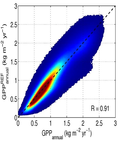
| R | 0.91 | 0.89 | 0.90 | 0.90 | 0.91 | 0.89 | 0.89 | 0.90 | 0.90 |
| MBE | 0.03 | −0.011 | −0.017 | −0.010 | −0.012 | −0.04 | −0.03 | 0.008 | −0.009 |
| MAE | 0.16 | 0.17 | 0.17 | 0.17 | 0.17 | 0.17 | 0.18 | 0.17 | 0.17 |
| RMSE | 0.2 | 0.2 | 0.2 | 0.2 | 0.2 | 0.2 | 0.2 | 0.2 | 0.2 |
| rMBE | 0.04 | −0.011 | −0.015 | −0.009 | −0.013 | −0.03 | −0.03 | 0.008 | −0.008 |
| rMAE | 0.18 | 0.17 | 0.15 | 0.16 | 0.17 | 0.16 | 0.17 | 0.18 | 0.17 |
| rRMSE | 0.2 | 0.2 | 0.2 | 0.2 | 0.2 | 0.2 | 0.2 | 0.2 | 0.2 |
| NDVI | |||||||||
| 1 | 2 | 3 | 4 | 5 | 6 | 7 | 8 | 9 | |
| C1 | −1.610 | −1.143 | −1.190 | −1.50 | −1.046 | −1.44 | −0.975 | −1.194 | −1.019 |
| (0.009) | (0.007) | (0.017) | (0.03) | (0.011) | (0.02) | (0.009) | (0.013) | (0.008) | |
| C2 | 5.682 | 4.164 | 4.20 | 4.68 | 3.561 | 4.40 | 3.302 | 4.15 | 3.62 |
| (0.018) | (0.018) | (0.03) | (0.04) | (0.019) | (0.04) | (0.017) | (0.02) | (0.02) | |
| EVI | |||||||||
| 1 | 2 | 3 | 4 | 5 | 6 | 7 | 8 | 9 | |
| C1 | −1.825 | −1.562 | −1.311 | −1.15 | −1.498 | −1.01 | −1.421 | −1.337 | −1.735 |
| (0.011) | (0.007) | (0.018) | (0.02) | (0.009) | (0.02) | (0.007) | (0.013) | (0.007) | |
| C2 | 7.99 | 6.68 | 6.25 | 6.15 | 6.95 | 5.77 | 6.319 | 6.25 | 7.29 |
| (0.03) | (0.02) | (0.04) | (0.05) | (0.03) | (0.06) | (0.017) | (0.03) | (0.03) | |
| NDVI | ||||||||||
| 1 | 2 | 3 | 4 | 5 | 6 | 7 | 8 | 9 | Global | |
| R | 0.75 | 0.90 | 0.89 | 0.83 | 0.79 | 0.83 | 0.75 | 0.89 | 0.84 | 0.90 |
| MBE | 0.0011 | −0.005 | 0.007 | 0.006 | −0.002 | −0.0003 | −0.013 | −0.004 | −0.013 | −0.007 |
| MAE | 0.3 | 0.13 | 0.18 | 0.2 | 0.18 | 0.2 | 0.2 | 0.16 | 0.16 | 0.17 |
| RMSE | 0.4 | 0.18 | 0.2 | 0.3 | 0.2 | 0.3 | 0.3 | 0.2 | 0.2 | 0.2 |
| rMBE | 0.0008 | −0.007 | 0.005 | 0.004 | −0.0017 | −0.00018 | −0.015 | −0.004 | −0.018 | −0.007 |
| rMAE | 0.2 | 0.16 | 0.13 | 0.15 | 0.15 | 0.12 | 0.2 | 0.15 | 0.2 | 0.16 |
| rRMSE | 0.3 | 0.2 | 0.18 | 0.19 | 0.2 | 0.16 | 0.3 | 0.2 | 0.3 | 0.2 |
| EVI | ||||||||||
| 1 | 2 | 3 | 4 | 5 | 6 | 7 | 8 | 9 | Global | |
| R | 0.76 | 0.90 | 0.90 | 0.84 | 0.81 | 0.85 | 0.80 | 0.90 | 0.87 | 0.91 |
| MBE | 0.005 | −0.009 | 0.0005 | 0.002 | 0.004 | −0.0019 | −0.007 | −0.006 | −0.008 | −0.009 |
| MAE | 0.3 | 0.13 | 0.18 | 0.2 | 0.17 | 0.18 | 0.19 | 0.16 | 0.14 | 0.16 |
| RMSE | 0.4 | 0.18 | 0.2 | 0.3 | 0.2 | 0.2 | 0.2 | 0.2 | 0.19 | 0.2 |
| rMBE | 0.004 | −0.011 | 0.0004 | 0.0015 | 0.004 | −0.0012 | −0.008 | −0.005 | −0.011 | −0.009 |
| rMAE | 0.2 | 0.16 | 0.13 | 0.14 | 0.14 | 0.11 | 0.2 | 0.15 | 0.19 | 0.16 |
| rRMSE | 0.3 | 0.2 | 0.18 | 0.18 | 0.19 | 0.15 | 0.3 | 0.19 | 0.3 | 0.2 |
| NDVI | EVI | |||
|---|---|---|---|---|
| Constant Values of C1 and C2 | C1 and C2 Values Depending on Vegetation | Constant Values of C1 and C2 | C1 and C2 Values Depending on Vegetation | |
| REFERENCE: GPPOPT | R = 0.87 | R = 0.90 | R = 0.90 | R = 0.91 |
| rRMSE = 0.3 | rRMSE = 0.2 | rRMSE = 0.2 | rRMSE = 0.2 | |
| rMBE = −0.008 | rMBE = −0.007 | rMBE = −0.009 | rMBE = −0.009 | |
| rMAE = 0.19 | rMAE = 0.16 | rMAE = 0.17 | rMAE = 0.16 | |
| REFERENCE: GPPMODIS | R = 0.87 | R = 0.87 | R = 0.84 | R = 0.86 |
| rRMSE = 0.3 | rRMSE = 0.3 | rRMSE = 0.3 | rRMSE = 0.3 | |
| rMBE = −0.07 | rMBE = −0.05 | rMBE = −0.07 | rMBE = −0.05 | |
| rMAE = 0.17 | rMAE = 0.16 | rMAE = 0.2 | rMAE = 0.18 | |
© 2017 by the authors. Licensee MDPI, Basel, Switzerland. This article is an open access article distributed under the terms and conditions of the Creative Commons Attribution (CC BY) license ( http://creativecommons.org/licenses/by/4.0/).
Share and Cite
Gilabert, M.A.; Sánchez-Ruiz, S.; Moreno, Á. Annual Gross Primary Production from Vegetation Indices: A Theoretically Sound Approach. Remote Sens. 2017, 9, 193. https://doi.org/10.3390/rs9030193
Gilabert MA, Sánchez-Ruiz S, Moreno Á. Annual Gross Primary Production from Vegetation Indices: A Theoretically Sound Approach. Remote Sensing. 2017; 9(3):193. https://doi.org/10.3390/rs9030193
Chicago/Turabian StyleGilabert, María Amparo, Sergio Sánchez-Ruiz, and Álvaro Moreno. 2017. "Annual Gross Primary Production from Vegetation Indices: A Theoretically Sound Approach" Remote Sensing 9, no. 3: 193. https://doi.org/10.3390/rs9030193
APA StyleGilabert, M. A., Sánchez-Ruiz, S., & Moreno, Á. (2017). Annual Gross Primary Production from Vegetation Indices: A Theoretically Sound Approach. Remote Sensing, 9(3), 193. https://doi.org/10.3390/rs9030193