Role of Climate Variability and Human Activity on Poopó Lake Droughts between 1990 and 2015 Assessed Using Remote Sensing Data

Abstract

In 2015, an emergency state was declared in Bolivia when Poopó Lake dried up. Climate variability and the increasing need for water are potential factors responsible for this situation. Because field data are missing over the region, no statements are possible about the influence of mentioned factors. This study is a preliminary step toward the understanding of Poopó Lake drought using remote sensing data. First, atmospheric corrections for Landsat (FLAASH and L8SR), seven satellite derived indexes for extracting water bodies, MOD16 evapotranspiration, PERSIANN-CDR and MSWEP rainfall products potentiality were assessed. Then, the fluctuations of Poopó Lake extent over the last 26 years are presented for the first time jointly, with the mean regional annual rainfall. Three main droughts are highlighted between 1990 and 2015: two are associated with negative annual rainfall anomalies in 1994 and 1995 and one associated with positive annual rainfall anomaly in 2015. This suggests that other factors than rainfall influenced the recent disappearance of the lake. The regional evapotranspiration increased by 12.8% between 2000 and 2014. Evapotranspiration increase is not homogeneous over the watershed but limited over the main agriculture regions. Agriculture activity is one of the major factors contributing to the regional desertification and recent disappearance of Poopó Lake.

1. Introduction

The recent drought at Poopó Lake, the second largest water body in Bolivia, is of major socio-environmental concern as it condemned local population dependent on fishing activities jointly with local endemic species. Moreover, the sediments contaminated by intense regional mining activities trapped in the lake bottom were exposed to wind erosion, threatening the Altiplano region with contamination. Thus, there is the necessity of providing efficient and consistent surface water monitoring tools for anticipating such crises and giving support for more sustainable use of water resource in this region. Two main factors can be pointed out to explain the recent lake total drought: global warming and water consumption increase. Actually, the region suffers from continuously increasing air temperatures of 0.15 to 0.25 °C over the last decades [1,2] from 1965 to 2012. This temperature increase has had a slight impact on evapotranspiration but has accelerated glacier melting [3]. Some glaciers already disappeared. For example, the Chacaltaya Glacier, which was one of the largest glaciers in the region, entirely melted in 2010 [4]. The shrinkage and disappearance of glaciers obviously reduces the replenishment of water resources (surficial and subterranean), especially during the dry season [5]. In addition to climatic factors, some anthropic factors may directly affect Poopó Lake. Water extraction to sustain increasing mining activity, human populations (for consumption) and agriculture kept rising over the last decades. Actually, the area of quinoa culture in Bolivia increased from 38,800 to 70,000 ha from 1990 to 2012 [6] in response to the world’s demands for quinoa and its increasing price. Progressively, the replacement of native vegetation by quinoa has accelerated the desertification process across the region [7,8]. As the outlet of its own watershed, the Poopó Lake extent fluctuation is sensitive to climate change and increasing anthropic water demands along the watershed. With more than 25 years of land observations using different spectral bands and considering replicates of 16 days, Landsat imagery collection is very suitable for monitoring variations in lake coverage and for support decision for more sustainable use of water resources in the future. However, the electromagnetic radiation signals collected by satellites in the solar spectrum are modified because they are scattered and absorbed by gazes and aerosols as they travel from the earth’s surface to the sensor. Atmospheric correction is arguably the most important step in pre-processing Landsat data to monitor change detection when considering multitemporal time series images [9,10,11] but not when working on single date [11]. Today, the United States Geological Survey (USGS) service provides an atmospherically corrected version of each LandSat scene: the Landsat Surface Reflectance (LSR) product. Here, we used field spectral measurement to quickly assess LSR estimates for the Landsat-8 OLI products for the first time over the Altiplano. The Surface Reflectances (SRs) obtained after applying the fast line-of-sight atmospheric analysis of spectral hypercubes (FLAASH) atmospheric correction were also considered for comparisons.

The method used to build a time series of the fluctuations of lake extent is based on detecting changes in the pixel’s state from one Landsat scene to another. In the literature, several satellite derived indexes (SDIs) are proposed to separate water and land pixels. Depending on the region, one SDI can be more suitable than another for delineating water bodies, and an SDI should be chosen carefully to produce realistic results [12,13]. However, in most studies, choosing the SDI remains arbitrary or is based on the results of studies conducted in supposedly similar regions [14,15,16,17]. Here, we compared the results obtained from the Normalized Difference Water Index (NDWI), Modified NDWI (MNDWI), Water Ratio Index (WRI), Normalized Difference Moisture Index (NDVI), Automated Water Extraction Index (AWEI), Normalized Burn Ratio (NBR) and Land Surface Water Index (LSWI) with field observations to provide general guidelines for potential users over the Altiplano region.

Finally, based on the most efficient Atmospheric model correction and SDI, a 26-year temporal series from 1990 to the 2015 disappearance of the lake is presented for the first time. After validation, the MOD16 evapotranspiration (ET) products, the Precipitation Estimation from Remotely Sensed Information Using Artificial Neural Networks–Climate Data Record (PERSIANN-CDR) and Multi-Source Weighted-Ensemble Precipitation (MSWEP) reanalysis rainfall products are confronted to the Poopó Lake extent fluctuations. Rainfall and ET general trends are used to understand the potential influence of the climatic variability and increasing irrigated quinoa culture over the watershed during the last decades. This study provides a preliminary analysis of the hydrological behavior of Poopó Lake over the last decades and could be used as a guideline by national authority to consider more sustainable use of water resources over the region.

2. Materials and Methods

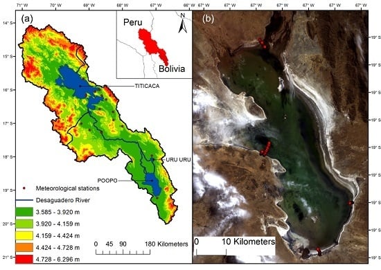
2.1. Study Area

Poopó Lake is located on the southern part of the Andean Plateau in Bolivia between latitudes 17°S and 20°S and longitudes 66°W and 68°W and with a mean elevation of 3686 m (Figure 1a). Poopó Lake is the second largest lake in Bolivia, covering an area of 500 to 3000 km² at its lowest and highest levels, respectively [17]. The extent of Poopó Lake drastically changes between wet and dry seasons because the region where the lake is located is very flat [18]. The only outflow of the lake is through the Lakajawuira River on the southern end of the lake, which rarely flows towards the Coipasa Salar. In the last 50 years, this river only flooded once in 1986 [17]. Thus, Poopó Lake is considered a terminal point of the endorheic Altiplano system [17]. The Poopó Lake region is arid, with a mean annual precipitation of approximately 400 mm over the lake [19] and a high evapotranspiration rate [20]. According to pan evaporation measurement, the potential evaporation was estimated at 1700 mm/year [17] and resulted in extremely saline water. Regarding the local population, the lake is of primordial importance because people depend on it for fishing and agricultural activities [7,8]. In December 2015, a national emergency alert was launched by the national authority in Bolivia after the lake totally dried up. This situation directly impacted the ecosystem and the population living around the lake.

2.2. Data Used

2.2.1. Field Spectral Measurements

Spectral radiometric measurements were acquired from the field, using TriOS RAMSES Sensors on 6 September 2014. A total of 69 points from 5 transects located on the north, east, south and west lakeshores and in the shallow part of the lake were analyzed (Figure 1b). At each point, the lake depth and SR in the spectral domain between 450 and 950 nm were registered. These data were acquired using the methodology established by [21]. Hereafter, we refer to Ground Control Points (GCPs) when referring to the in situ measurements. Spectral radiometric and Landsat measurement differ in term of spatial resolution (point vs. Pixel). This is an important feature to be considered to avoid inconsistent comparison. To account for this, spectral radiometric measurements were done on homogeneous area in term of water depth and water–soil representation to avoid mixed pixel. As Poopó region is a very flat region, and Landsat pixel length is of approximately 30 m, it was easy to find homogeneous areas all around the lake. Recorded values were resampled to match Landsat OLI 8 blue, green, red and near infra-red (NIR) bands. The Landsat Quality Assessment (QA) band provides the bit-packed values of the surface, atmosphere and sensor conditions that can affect the reflectance measured at each pixel of the considered scene. According to the QA band, 13 points were dismissed because of clouds or cirrus cover and 56 points were available for comparisons. Landsat reflectance measurements are given per unit area, while TriOS RAMSES measurements provide reflectance values per unit solid angle (Steradian). Thus, field spectral measurements were multiplied by the π value to match the Landsat reflectance value.

2.2.2. Landsat Imagery

The Landsat-8 satellite was launched in February 2013 with OLI and Thermal Infra-Red Sensor (TIRS) instruments on board. OLI, ETM+, ETM and TM sensors have different bandwidths that could compromise their compatibility. Regarding the OLI and ETM+, good radiometric compatibility was found between their respective bands [22] and can be used as complementary data [23]. OLI was found to largely inherit the band-pass characteristics of ETM+ and achieve continuity of Landsat data [24]. On the other hand, TM and ETM + were found to exhibit excellent data continuity [25], and the measurements of SR obtained by these sensors could be combined with minimal error without sacrificing product accuracy [26,27,28]. Based on these observations, it is possible to use OLI, ETM+ and TM jointly to retrieve long temporal series or series with increased observation frequencies. Each Landsat scene is available in an atmospherically corrected format called the LSR product and freely available from the USGS. For the Landsat TM, ETM and ETM+, the specialized Landsat Ecosystem Disturbance Adaptive Processing System (LEDAPS) software [29] and the specialized L8SR software [30] are used to retrieve the SR for Landsat TM, ETM and ETM+ and Landsat-8 OLI, respectively.

2.2.3. Satellite Rainfall Estimates

Two reanalysis rainfall products named PERSIANN-CDR [31] and MSWEP [32] were considered to cover the whole 1990–2016 period. PERSIANN-CDR was released in 2014 by the National Climatic Data Center (NCDC) Climate Data Record (CDR) program of the National Oceanic and Atmospheric Administration (NOAA). PERSIANN-CDR covers the 1983 to 2015 period providing daily rainfall estimate on a 0.25° spatial resolution. MSWEP was released in 2016 [32] and covers the 1979–2015 period with daily rainfall data on a 0.25° spatial resolution. MSWEP estimates are based on the Climate Hazards Group Precipitation Climatology (CHPclim) dataset (0.05°) [33]. Additionally, precipitation anomalies from gauge observation, satellite rainfall estimates and atmospheric model reanalysis are used to fix MSWEP estimates temporal variability.

2.2.4. MOD16 Global Evapotranspiration

MOD16 global evapotranspiration is a product of NASA. Estimates are made according to an algorithm based on Penman–Monteith equation [34,35]. NASA’s MERRA GMAO (GEOS-5) daily meteorological reanalysis data are used to retrieve radiation, air pressure, temperature and humidity. MODIS products are used to retrieve complementary data on an 8 days temporal scale. MOD12Q1 collection 4 is used for the land cover classification [36], MOD15A2 collection 5 to retrieve Leaf Area Index (LAI) and Fraction of Photosynthetically Active Radiation (FPAR) [37] and MCD43B2/B3 Collection 5 are necessary to get albedo estimates [38]. Four products are available: Potential Evapotranspiration (ETp), Real Evapotranspiration (ETr), Latent Heat Flux (LE) and Potential Latent Heat Flux (PLE). All products are available in a 0.05 grid resolution at 8 days and monthly temporal scale. In this study, we used monthly MOD16 ETp and ETr from January 2002 to December 2014.

2.3. Methods Used

2.3.1. FLAASH Atmospheric Correction

The Landsat-8 OLI scene of 6 September 2015 was used to implement the atmospheric correction process. First, we converted the image from digital numbers to top of atmosphere (TOA) radiance by using pre-processing tools in ENVI v.5.2. Then, the FLAASH model, which is available in ENVI v.5.2, was used to transform the TOA value to land SR. FLAASH used the MODTRAN4 radiation transfer code [39], which was modified to correct errors in the HITRAN-96 water line parameters. Multispectral imagery, such as Landsat imagery, does not include water absorption bands. Instead, a constant amount of water vapor is set for all pixels of the scene according to an atmospheric model. Depending on the water vapor content, different atmospheric models are available. Here, by using MOD_D3_008 (Modis Level 3 Atmospheric products), we observed a vapor content of 2.15 g/cm² on the date of the Landsat-8 OLI observation. This value corresponds to the water vapor content that is advisable for the Sub-Artic Summer (SAS) atmospheric model [40]. Thus, this model was used to run FLAASH. The rural aerosol model was selected according to the regional context, with an initial visibility of 25 km, which is recommended when moderate haze is observed (Figure 1b). Finally, the elevation of the field was fixed at 3.8 km, which was the approximate value of the elevation observed over Poopó Lake. Hereafter, the atmospheric corrected image is referenced to as FLAASH after the SAS model was applied.

2.3.2. Satellite-Derived Indexes for Water Extraction

Various SDIs exist for separating water bodies from land. Here, the NDWI, MNDWI, WRI, NDVI, AWEI, NBR and LSWR were considered over the Poopó Lake region. The equations and threshold value indexes are reported in

Table 1. Satellite-derived indexes used for extraction.

Index	Equation	Threshold Value
Normalized Difference Water Index	NDWI = (Green − NIR)/(Green + NIR)	Water > 0
Modified Normalized Difference Water Index	MNDWI = (Green − SWIR1)/(NIR + SWIR1)	Water > 0
Water Ratio Index	WRI = (Green + Red)/(NIR + SWIR1)	Water > 1
Normalized Difference Vegetation Index	NDVI = (NIR − Red)/(NIR + Red)	Water < 0
Automated Water Extraction Index	AWEI = 4 × (Green − SWIR1) − (0.25 × NIR + 2.75 × SWIR2)	Water > 0
Normalized Burn Ratio	NBR = (NIR − SWIR2)/(NIR + SWIR2)	Water > 0
Land Surface Water Index	LSWI = (NIR − SWIR1)/(NIR + SWIR1)	Water > 0

and are detailed in [12,23].

2.4. Assessment of Data and Method

2.4.1. L8SR and FLAASH Assessment

At each GCPs location, field spectral measurement, FLAASH, LSR and Landsat SR value for Blue, Green, Red and NIR were extracted to build the database. Comparisons between field spectral measurement and FLAASH, LSR and Landsat SR were made considering all single band values (red, blue, green and near infra-red) and possible band ratios (green/red, blue/green, red/blue, blue/near infra-red, green/near infra-red, and red/near infra-red) (

Table 2. %ME, %RMSE and CC for the SR measured by Landsat (uncorrected), FLAASH SAS and LSR in comparison with in situ field measurements.

	ME (%)			RMSE (%)			CC
	Landsat	FLAASH	LSR	Landsat	FLAASH	LSR	Landsat	FLAASH	LSR
Blue	0.0	−0.9	−0.9	48.4	109.2	110.9	0.92	0.93	0.91
Green	−0.2	−0.9	−0.9	44.0	102.7	103.7	0.91	0.92	0.91
Red	−0.2	−0.9	−0.9	45.2	103.4	104.0	0.91	0.91	0.91
Near IR	−0.1	−0.9	−0.9	57.8	115.1	115.6	0.84	0.84	0.84
Green/Red	0.0	0.0	0.0	13.1	5.0	6.5	0.94	0.98	0.97
Blue/Green	0.4	0.1	0.0	38.6	9.4	12.4	0.47	0.88	0.69
Red/Blue	−0.3	0.0	0.0	41.9	10.9	15.6	0.75	0.96	0.89
Blue/Infra-Red	−0.5	−0.1	−4.0	122.1	46.3	2663.3	0.90	0.93	−0.35
Red/Infra-Red	−0.6	−0.1	−3.8	118.5	45.3	2512.3	0.87	0.92	−0.37
Green/Infra-Red	−0.7	−0.1	−4.4	137.2	50.1	2896.3	0.88	0.93	−0.38

). Landsat reflectance value was considered to observe the enhancements of the SR estimations gained through the L8SR and FLAASH processes. The band ratios are considered to observe the relative errors between bands. Indeed, low error in band ratio implies that the trend between the concerned bands is well represented. Considering all GCPs, the Mean Error (ME), Root Mean Square Error (RMSE) and Correlation Coefficient (CC) were computed for all single and band ratios. Different ranges of values were observed for the different bands and band ratios, which complicated the interpretation of the absolute errors. Thus, the ME and RMSE were divided by the average GCP value to obtain the relative statistic error percentage (%ME and %RMSE) (Table 2).

2.4.2. SDI Assessment

Poopó Lake is a very shallow lake. In shallow part, light penetration in water column is very high. Thus, SR is highly influenced by Lake Bottom response complicating water/land separation. To account for this feature, we divided the GCPs into 4 classes corresponding to “water”, “very shallow water”, “interconnected water”, and “soil”. The classes contained 26, 16, 5 and 9 GCPs, respectively. The “Very shallow water” and “water” classes had water depths ranging from 0 to 5 cm and superior to 5 cm, respectively. The “interconnected water” class corresponded to mixed pixels with interconnected water units. At each pixel location, including a GCP, the SDI values from the most accurate scenes in term of the SR estimation were compared with field observations. Two cases are possible: SDI value and field observations agreed or SDI value and field observations disagreed (

Table 3. Assessment of SDI over Poopó Lake. Water refers to “water” and “very shallow water” classes, and Land refers to “interconnected water” and “soil” classes.

		SDI Observation
		Water	Land
Field Observation	Water	Ok	Outlier
	Land	Outlier	Ok

). Outlier values were observed when the SDI failed to correctly identify the field observations (Table 3, Figure 2). A large number of outliers mean that the considered SDI was poorly efficient over the region. SDIs potentiality is generally more effective after the threshold value was adjusted. Here, for each considered SDI, we proposed an adjusted threshold to minimize as possible the outlier number. For each SDI, the number of outliers was computed before and after the threshold adjustment (

Table 4. SDI outliers for the default and adjusted threshold values with the corresponding superficial extents of Poopó Lake on 22 September 2014.

SDI	Default Threshold Value	Outlier Number	Superficial (km2)	Recommended Threshold Value	Outlier Number	Superficial (km2)
NDWI	0	14	1204	−0.0235	12	1314
MNDWI	0	6	1664	0.15	3	1477
WRI	1	4	1570	1.05	3	1497
NDVI	0	7	1160	0.025	6	1208
AWEI	0	4	1454	−0.1	3	1454
NBR	0	13	2627	0.21	7	1906
LSWI	0	10	2099	0.05	6	1820

). Finally, we computed the extent of Poopó Lake based on each SDI using the default and adjusted threshold values (Table 4).

2.4.3. Satellite Rainfall and MOD16 Evapotranspiration Estimates Assessment

The mean regional monthly rainfall series was computed for both PERSIANN-CDR and MSWEP for the 1998–2014 period aggregating all pixels included into the watershed. Another mean regional monthly series was computed by meaning PERSIANN-CDR and MSWEP rainfall series (called MERGE hereafter). The three series were compared to a mean reference regional monthly series derived from the Multisatellite Precipitation Analysis 3B42 (TMPA-3B42) v.7 for the same period. TMPA-3B42 v.7 can be used as reference as it was found suitable over the region to describe monthly rainfall events [19]. The accuracy of PERSIANN-CDR, MSWEP and MERGE monthly rainfall estimates were assessed considering Correlation Coefficient (CC) and Bias (Figure 3a).

Real Evapotranspiration (ETr) measurement requires specifics sensor that are not available over the region. Thus, direct comparison between reference and MOD16 ETr are not possible. ETp is easily measurable from meteorological variables. Over the region, ETp derived from Thornthwaite, Hargreaves–Samani and FAO Penman–Monteith equations were compared with ETp derived from lysimiters measurement [20]. According to the authors, Penman–Monteith equations can be used to represent ETp. Following FAO Penman-Monteith equation (Equation (1)) we computed monthly ETp at the location of 16 meteorological stations (Figure 1a) for the period 2002–2010. The equation uses standard climatological records of solar radiation, air temperature, humidity and wind speed.

$$ETp=\frac{0.408\mathrm{\Delta }\left(Rn-G\right)+\gamma \times \left(\frac{900}{T+273}\right)\times U_2\times \left(E_s-E_a\right)}{\mathrm{\Delta }+\gamma \times \left(1+0.34\times U_2\right)}$$

(1)

where ET_p is the reference evapotranspiration (mm·day⁻¹), R_n is thenet radiation at the crop surface (MJ·m⁻²·day⁻¹), G is the soil heat flux density (MJ·m⁻²·day⁻¹), T is the mean daily air temperature at 2 m height (°C), U₂ is the wind speed at 2 m height (m·s⁻¹), E_s is the saturation vapor pressure (kPa), E_a is the actual vapor pressure (kPa), $\mathrm{\Delta }$ is the slope vapour pressure curve (kPa·°C⁻¹), and $\mathsf{\gamma }$ is the psychrometric constant (kPa·°C⁻¹).

At each of the 16 stations location, the monthly ETp was derived from both the meteorological station and the corresponding MOD16 pixel. Finally, two mean monthly ETp series were derived by aggregating values obtained from the 16 meteorological stations and corresponding MOD16 pixels, respectively. ETp derived from meteorological station is considered as reference ETp (denoted RETp, hereafter). MOD16 ETp and RETp mean monthly series were compared considering CC and Bias (Figure 3b). Finally, MOD16 ETr accuracy is assumed to be similar to MOD16 ETp accuracy.

2.5. Temporal Analysis

2.5.1. Rain versus Superficial Lake Area

From January 1990 to December 2015, the annual highest and lowest lake extents were derived for each year from Landsat imagery by using the most efficient previously identified atmospheric correction processes and SDI. Attention was paid to only select almost cloud free Landsat TM, ETM or OLI scenes. Overall, 48 Landsat scenes were selected and used. From 2012, only Landsat ETM+ scenes are available. Over Poopó Lake, the Landsat ETM+ scenes are strongly impacted by the SLC failure that occurred on 31 May 2003. Thus, these data are not suitable for use in the study. Therefore 2 MODIS scenes were used to fill the gap. Using the MODIS scene to derive the extent of Poopó Lake is acceptable because a strong correlation was previously found between the extents of Poopó Lake derived from MODIS and Landsat data [14]. MODIS scenes are already atmospheric corrected and thus SDI can be directly applied. The fluctuation of the lake extent was compared with the mean regional annual rainfall evolution (Figure 4a). The mean rainfall was computed based on a hydrological year (November to October) and using MERGE rainfall product (Figure 4a). Additionally, the mean seasonal rainfall anomalies and lake extent anomalies for both dry and wet seasons were computed and compared (Figure 4b).

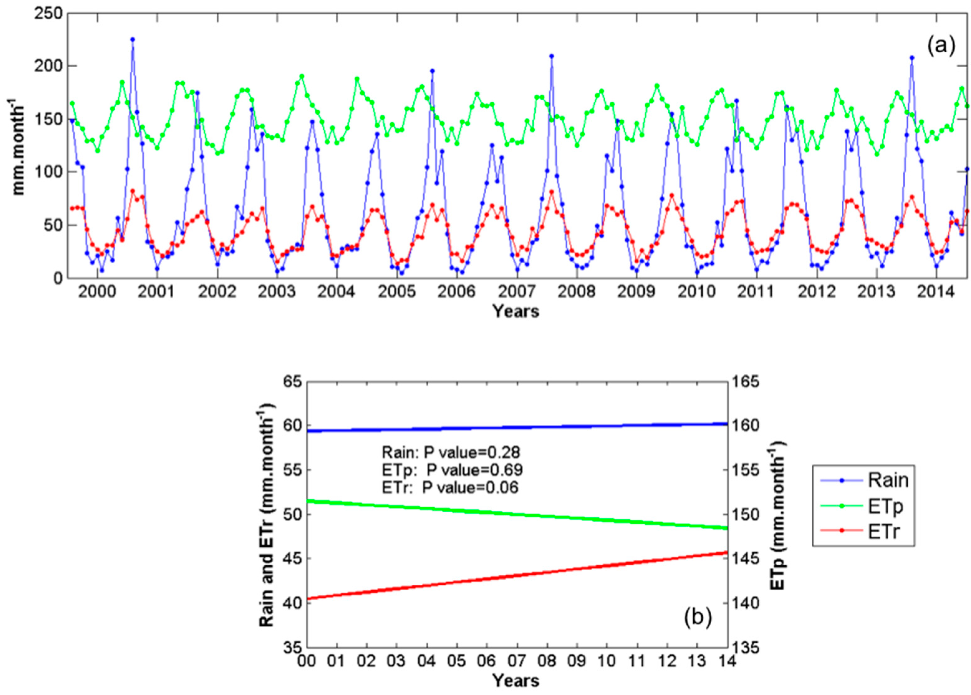
2.5.2. ETr, ETp and Rainfall Tendency over the Last 15 Years

The monthly rainfall, ETp and ETr over Poopó Lake watershed for the period 2000–2014 are presented jointly with their global trend (Figure 5). The global trend is obtained from a simple linear regression of the mean monthly series. The Mann-Kendall (MK) test [41,42] was used to statistically verified if the monotonic trend in the mean monthly rainfall, ETp and ETr over the 2000–2014 period were significant. A MK p-value inferior to 0.05 corresponds to significant monotonic trend. Finally, to observe the ETr dynamic in space along the whole watershed, the mean monthly ETr series were computed at each MOD16 pixel location and its linear regression was used to compute the ETr changing rate from 2000–2014 (Equation (2)). Results are presented in Figure 6. Additionally, the MK p-value was computed at each MOD16 pixel according to the corresponding ETr series. Results are presented in Figure 6.

$$ChangingRate=\frac{\left(ET{r}_{2014}-ET{r}_{2000}\right)\times 100}{ET{r}_{2000}}$$

(2)

where ETr₂₀₁₄ and ETr₂₀₀₀ are the ETr computed from the linear regression of the considered MOD16 pixel for the years 2014 and 2000, respectively.

Finally, a multiple linear regression was used to check the relative influence of rain, ETp and ETr on the lake fluctuations for the 2000–2014 period. The annual lake extent during the dry season was considered as dependent variable while corresponding mean regional annual precipitation, ETp and ETr were considered as independent variables (predictors). The mean annual precipitation, ETp and ETr were computed for the corresponding season between May and March. It is noteworthy that we only considered lake extent fluctuation during the dry season. Actually, the lake extent during the wet season is controlled at 65% by Desaguadero River input and the rest by local Poopó Lake watershed input [17]. Thus, at the regional scale, the influences of rain, ETp and ETr are expected to be more significant during the dry season than during the wet season as Desaguadero River input is much smaller.

3. Results and Discussion

3.1. Effects of Atmospheric Correction

Using a single band approach and for all considered bands, the Landsat SR estimate was generally closer to the field SR measurements than the LSR and FLAASH SR with %ME and %RMSE close to 0. FLAASH and LSR resulted in underestimations of SR with negative bias values. When considering the band ratio, the FLAASH and LSR SR estimations were closer to the field SR than the Landsat SR estimates with %ME closer to 0 and lower RMSE value. The corrected LSR and FLAASH data tended to result in more homogeneous relative trends between the bands than the uncorrected data. Indeed, for all band ratios, the error distribution was closer to 0 for the LSR and FLAASH scenes than for the Landsat scene, which presented greater error distributions.

The NIR band is the most affected by atmospheric absorption and scattering. This band presented lower CCs and higher %RMSEs and %MEs. Consequently, all band ratios including the NIR band presented highest %RMSE values (Table 2). In the case of FLAASH correction, the %RMSE was 5–10 times higher than that of the other ratio (Table 2). This difference was even greater when considering the LSR products with very high %RMSEs for the band ratios including the NIR band. This difference results from the strong underestimation of the NIR with some negative value observed. This LSR inconsistency seems to reoccur because negative values in NIR bands were also observed in the LSR scenes from 21 August and 22 September 2014 as well as over Brazilian water bodies at different date. Although FLAASH also underestimates the NIR SR value, it had a lower impact because no negative value was observed.

Using the single band approach, atmospheric correction degraded the SR estimation because lower %ME and %RMSE values were found before atmospheric correction was applied. However, the opposite trend was observed when considering the band ratios. FLAASH Atmospheric correction enhanced the relative error between the bands, with %RMSE reduction by a factor of 3, higher CCs and lower %MEs for all of the considered band ratios. Thus, over Poopó Lake, FLAASH correction is more suitable than the L8SR algorithm. SDIs are based on band combination and thus their efficiency highly relies on relative band error. As the study aimed to use SDI to retrieve lake extent, we used the FLAASH correction to build the Landsat scene database for the 1990–2015 period.

3.2. SDI Assessment

SDIs were computed for the Landsat-8 OLI scene of 6 September 2015 after the FLAASH correction was applied because it provided better SR estimations. Among the considered indexes, NDWI, NBR and LSWI were the least suitable SDIs for the region, with 14, 13 and 10 outliers, respectively (Figure 2; Table 4). The NDVI, MNDWI, AWEI, and WRI were the most efficient indexes, with only 7, 6, 4, and 4 outliers, respectively. To provide more insights from our results, we considered that outliers located in a dry soil or water pixel were more “problematic” than the outliers located in interconnected water pixels. Indeed, it is difficult to assess the performances of SDIs when considering mixed pixels as the SDI estimates are clearly dependent on the water: soil ratio, and the pixels should be classified based on the dominant component, water or soil. The NDVI, MNDWI, AWEI, and WRI have 7, 2, 1 and 1 “problematic” outliers, respectively (Figure 2). Before any threshold adjustment, the AWEI and WRI are the most efficient SDIs over Poopó Lake. The NDVI and NDWI are not very accurate over the very shallow lake regions, which are misclassified as soil (Figure 2). Thus, using NDVI or NDWI would considerably underestimate the extent of Poopó Lake which is confirmed by the lower extent of Poopó Lake derived from the NDVI and NDWI (Table 4). NBR and, to a lesser extent, LSWI provided the highest extents (Table 4) because they tended to classify all the GCPs as water. The MNDWI, AWEI and WRI provided similar estimations of the extent of Poopó Lake.

According to Figure 2, it is possible to adjust the recommended threshold to enhance the performances of the SDIs. The adapted threshold values for each SDI are shown in Table 4 with the corresponding numbers of outliers. The threshold adjustment decreased the number of outliers for all the SDIs leading to closer lake extent estimate between them. Finally, the MNDWI, AWEI and WRI perform equally, with similar estimated water extents and should be chosen to estimate Poopó Lake extent. For comparison, in a similar context, over the hyper saline Lake Urmia of Iran, the NDWI was the most suitable SDI for retrieving the spatiotemporal extent of the lake [12]. The different observed results show the relevance of such assessments for selecting the most suitable SDIs over a considered region.

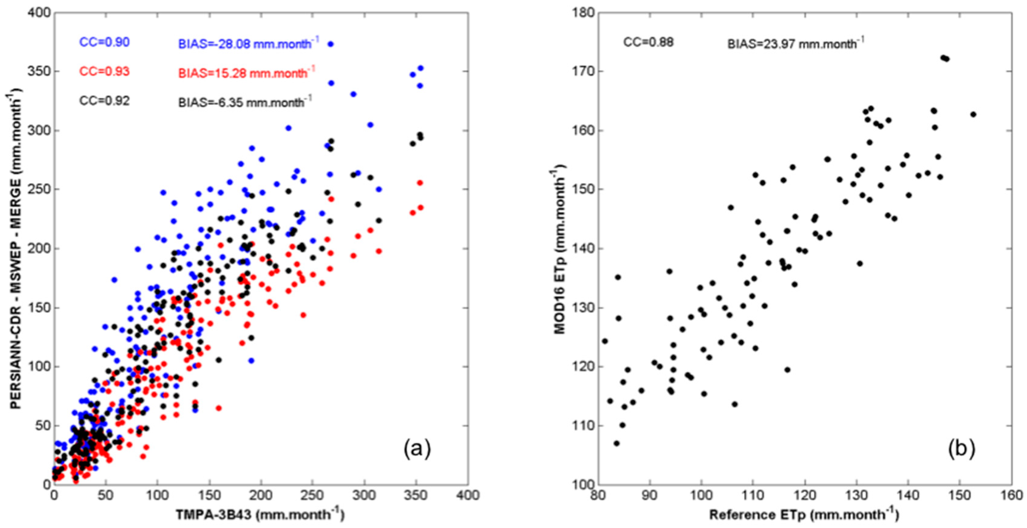
3.3. Satellite Rainfall and MOD16 Evapotranspiration Estimates

Among PERSIANN-CDR, MSWEP and MERGE rainfall estimates, and for the 1998–2014 period MERGE have the lowest Bias and close to highest CC (Figure 3a). MERGE product achieved to represent monthly rainfall over the study area and was selected for the study. A good agreement was found between MOD16 ETp and reference ETp estimates with a CC value of 0.88 and a mean Bias value of 23.97 mm·month⁻¹ (Figure 3b). As all involved meteorological factors to retrieve ETp are also involved in ETr computation, MOD16 ETp accuracy is highly representative of MOD16 ETr accuracy. Here, we consider MOD16 ETr suitable to describe ETr fluctuation over the region for the period 2000–2014.

3.4. Rainfall versus the Superficial Extent of the Lake

To verify the fluctuations of lake extent with time, we visually compared the fluctuations against the annual amounts of rainfall derived from the MERGE product from January 1990 to December 2015. This comparison included a preliminary approach for understanding the possible factors that affected the drought in Poopó Lake in December 2015.

Maximum lake extents of 2492 km², 2333 km² and 2256 km² were retrieved from multispectral scenes obtained on 31 March 1991, 3 April 2001, and 6 April 2012, respectively. The minimum extents of the lake of 432, 581 and 669 km² were observed for 20 October 1995, 22 October 1996, and 14 December 2015, respectively. However, the local population and press indicated that the lake totally dried up in December 2015 (National Geographic, 2016; Earth Observatory, 2016). Thus, according to our results, Poopó Lake should be considered as dried up when its extent is less than 700 km² because it becomes too shallow to sustain fish life. Thus, during 1990–2015 Poopó Lake dried up three times, in 1994, 1995 and 2015.

Very low extents of 776, 836 and 846 km² were also observed on 15 December 1998, 11 October 2008, and 13 December 2009, respectively. For comparison, the lake was observed to dry up in 2009 in a previous study and to nearly dry up in 2008 and 2010 [14]. However, according to local populations, the lake did not completely dry up on these dates. This might be due to the water masked approach used. This study used different methods that were partially based on the NDWI, which is one of the less accurate SDIs according to our results underestimating the superficial extent of Poopó Lake. One interesting feature of our analysis is the presence of a “critical” threshold value of approximately 1500 km². Each time the lake passed below this extent during the wet season, the extent of the lake decreased drastically during the following dry season and reached a very critical level, which occurred in 1995, 1996, 1998, 2008, 2009, 2010 and 2015 (Figure 4a). The annual variation between the extents of the lake during high and low water periods was much more defined during these years than the others (Figure 4a). This result could be helpful for anticipating when the lake will dry up during periods of low water.

From 1990 to 1996, the Lake extent during the wet and dry seasons steadily decreased in response to low rainfall amount with strong rainfall negative anomalies in 1991 and 1994 years. From 1996 to 2001, the Lake extent globally increased alternating increase and decrease period associated to positive and negative rainfall anomalies (Figure 4b). From 2001 to 2010, the Lake extent during the wet and dry seasons steadily decreased while the recorded annual rainfall steadily decreased from 2001 to 2004 to remain lower than or close to the mean from 2006 to 2010 (Figure 4b). During the last studied period of 2011 to 2015, the Lake extent during the wet and dry seasons dramatically decreased although the amount of annual rainfall was superior to the mean. For the first time, high positive rainfall anomalies (2013–2014 and 2014–2015) were observed in association with negative Lake extent anomalies (Figure 4b). Thus, during the last decades, our results suggest that the amount of water entering the lake from other water sources, mainly groundwater and the Desaguadero River, decreased. Actually, the Desaguadero discharge decreased 42%–54% between the periods of 1960–1990 and 1990–2008 [43]. This discharge reduction potentially had an obvious impact because the river is known to contribute 65% of the total water that enters Poopó Lake [17]. Some anthropic and climatic factors may have non-negligible impacts.

3.5. ETp, ETr and Rainfall Analysis

Figure 5a presents ETp, ETr and rain monthly series for the 2000–2014 period. The seasonal cycle is observed with highest ETp, ETr and rain during the wet season. With rainfall superior to ETr, wet seasons refill hydric resources (Figure 5a). On the contrary, during dry seasons, ETr is superior to rainfall corresponding to a hydric stress period. The annual rainfall amount estimated as 715 mm·month⁻¹ hardly compensates for the annual ETr amount estimated at 520 mm/year for the period of 2000–2014. Therefore, Poopó Lake is particularly sensitive to any upstream changes in precipitation and ETr conditions.

At the watershed scale, ETr increased from 43.8 to 48.3 mm·month⁻¹ between 2000 and 2014 with a mean increase rate of 12.8%. The MK p-value of 0.06 is slightly superior to the significant threshold value fixed to 0.05 (Figure 5b). This is related to the non-homogenous ETr increase along the watershed (Figure 6). Two hotspot regions with ETr increase rate superior to 15% were observed in the northern and southern part of Lake Titicaca, respectively (Figure 6). The increase rates observed in those regions are significant with MK p-value inferior to 0.05 (Figure 6). Those two regions correspond to intensive agriculture regions. A third region with significant ETr increase trend from 5% to 10% (MK p-value < 0.05) was observed on the eastern part of Poopó Lake (Figure 6). This region is also concerned by an increase in Quinoa crop. The regions where ETr is the most significant correspond to the main agriculture spots. It confirms the desertification processes previously suggested by [7,8] in relation to the replacement of native vegetation by crop (especially Quinoa).

However, climate variability should have participated to ETr increase as well. For example, the temperature increased by 0.15 to 0.25°C·decades⁻¹ over the 1965 to 2012 period [1]. ETp and ETr involved the same climatological factor for their estimation. Thus, if climatologic variability played a role in the ETr increase, ETp should have increase as well. However, over the 2000–2014 period and considering the whole watershed, no significant trend was observed on the mean monthly ETp with a MK p-value of 0.69 (Figure 5b). Additionally, no significant trend was found for mean monthly precipitation either, with a MK p-value of 0.28 (Figure 5b). Therefore, the observed ETr increase is more related to the agriculture activities than to climate variability. The replacement of traditional manual cultivation by mechanized system, the reduction of fallow period and the use of irrigation processes facilitate water availability for ETr processes. In the last several decades, new irrigation projects were set up along the Desaguadero River; however, no information regarding the amount of water extracted for irrigation is available. Peruvian and Bolivian Government should consider more reasonable agricultural methods to avoid the desertification process of the region. Currently, such scenario should considerably decrease agriculture yield leading to an economic disaster over the region.

Finally, the respective influences of ETp, ETr and precipitation trends on Poopó extent fluctuation and the recent drought were assessed by multiple linear regression. The results show a significant p-value of 0.048 for ETr while both ETp and Rainfall presented insignificant p-value > 0.05. Thus, the recent decrease of Poopó Lake extent observed during the last 14 years appears to be more related to ETr increase than to precipitation and climate fluctuation (ETp). However, this observation has to be considered with caution due to the small number of points used (14). Therefore, more consistent analyses based on longer temporal series have to be considered in future studies to definitively state the role of ETr on the Poopó Lake drought.

4. Conclusions

In this study, a guideline to monitor Poopó Lake extent variation in time from remote sensing data is presented to understand its recent disappearance. Landsat imagery was used to retrieve Poopó Lake extent and PERSIANN-CDR, MSWEP and MOD16 data were used to understand Poopó Lake extent variation in time at seasonal and annual scales in relation to climate variability and agricultural activities.

The first step consisted of a quick assessment of atmospheric correction, SDIs to retrieve Poopó Lake extent, reanalysis satellite rainfall products (PERSIANN-CDR and MSWEP) and MOD16 ET products at a monthly scale. Despite the scarcity of the ground reference, some consistent features emerged from the analysis:

(1)

More accurate SR values are obtained after the FLAASH correction was applied on the Landsat scene than from the already atmospheric corrected LSR scene. One positive effect of both atmospheric correction methods is the decrease of the relative error between the bands. This effect is even more pronounced when considering SR derived from the FLAASH correction with lower %RMSE, %ME values and higher CC values for all the considered band ratios. Thus, FLAASH is recommended to pre-process Landsat imagery rather than the use of LSR product.

(2)

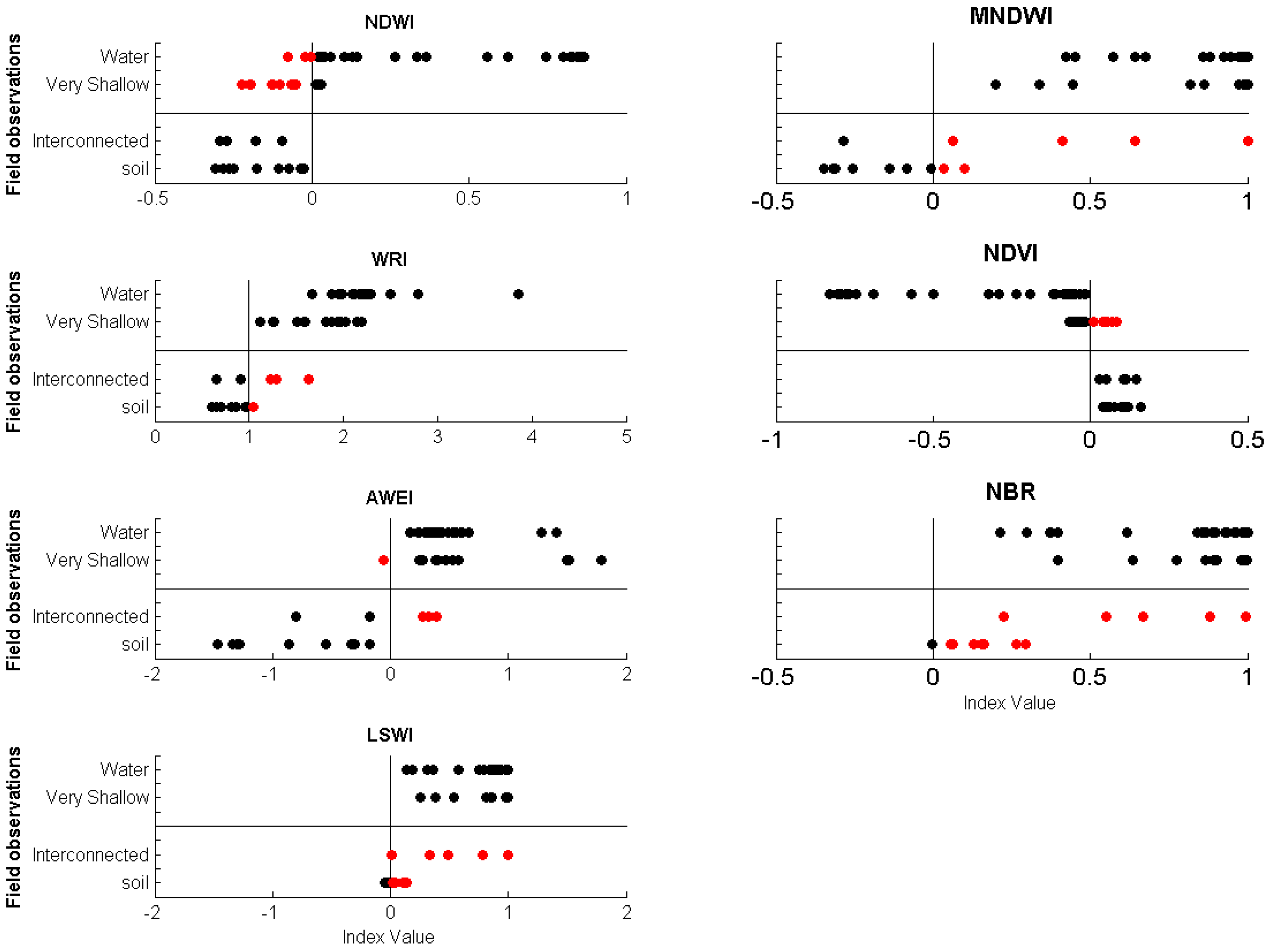
The AWEI, WRI and MNDWI were the most accurate SDIs over the region and only failed to classify mixed water and soil pixels. The NDVI and NDWI classified the shallower lake region as soil, which considerably underestimated the extent of Poopó Lake. The proposed threshold adjusted values enhance all SDIs efficiencies.

(3)

The two rainfall reanalysis products, PERSIANN-CDR and MSWEP, are accurate enough to represent regional monthly rainfall amount. Thus, using PERSIANN-CDR with MSWEP, the proposed MERGE monthly rainfall amount is even more suitable with a very low mean monthly bias value.

(4)

The low bias and high CC observed comparing MOD16 and reference ETp suggest that MOD16 ETr is accurate enough to represent regional monthly ETr.

Secondly, thanks to 26 years of common data acquisition of Landsat and MERGE rainfall data, preliminary insights regarding the fluctuations of Poopó Lake during the last decades are discussed. The extent of the lake passed by three maximum extents in 1991, 2001 and 2012 with lake extent of 2492 km², 2333 km² and 2256 km², respectively. Considering the recent dry extent of December 2015, it appears that Poopó Lake already dried up in 1994 and 1995, which are associated with strong negative rainfall anomalies. However, in 2014 and 2015, two high positive rainfalls are observed while lake extent drastically decreased until the lake dried up in December 2015. This observation suggests that outside factors influenced the recent disappearance of the lake. Various hypotheses can be made regarding the effects of global warming, which has resulted in the shrinkage and disappearance of some glaciers in the region. In addition, the increase of quinoa culture, mining activity and population water consumption potentially played roles in the disappearance of the lake. Consequently, a discharge decrease of 50% over the last 50 years is observed on the Desaguadero River which contribute 65% of the total water to Poopó Lake [17].

The analysis of ETr reveals an increase of approximately 12.8% at the watershed scale for the 2000–2014 period. The increase of ETr is not homogeneous over the region but located over the three main agricultural regions around Lake Titicaca and Poopó Lake. In those regions, the surface dedicated to quinoa crop kept rising over the last decades in response to a world demand and irrigation processes are involved to improve yield. Consequently, the local ETr over those regions drastically increased at a rate superior to 15% over the 2000–2014 period. Therefore, the agricultural activity and irrigation project from the Desaguadero River must be rigorously controlled before the total desertification of the region. In this line, according to this study, a minimum water extent of 1500 km² at the end of the rainy season is recommended to avoid allowing the drying up of the lake during the following dry season. National authorities should consider this threshold as an objective agreement to preserve the region from desertification while maintaining quinoa culture and the economic benefit it generates.

References

1. López-Moreno, J.I.; Morán-Tejeda, E.; Vicente-Serrano, S.M.; Bazo, J.; Azorin-Molina, C.; Revuelto, J.; Sánchez-Lorenzo, A.; Navarro-Serrano, F.; Aguilar, E.; Chura, O. Recent temperature variability and change in the Altiplano of Bolivia and Peru. Int. J. Clim. 2015. [Google Scholar] [CrossRef]
2. Seiler, C.; Hutjes, R.W.A.; Kabat, P. Climate variability and trends in Bolivia. J. Appl. Meteorol. Climatol. 2013, 52, 130–146. [Google Scholar] [CrossRef]
3. Bradley, R.S.; Vuille, M.; Díaz, H.F.; Vergara, W. Threats to water supplies in the tropical Andes. Science 2006, 312, 1755–1756. [Google Scholar]
4. Rabatel, A.; Francou, B.; Soruco, A.; Gomez, J.; Cceres, B.; Ceballos, J.L.; Basantes, R.; Vuille, M.; Sicart, J.E.; Huggel, C.; et al. Current state of glaciers in the tropical Andes: A multi-century perspective on glacier evolution and climate change. Cryosphere 2013, 7, 81–102. [Google Scholar] [CrossRef] [Green Version]
5. Juen, I.; Kaser, G.; Georges, C. Modelling observed and future runoff from a glacierized tropical catchment (Cordillera Blanca, Perú). Glob. Planet. Chang. 2007, 59, 37–48. [Google Scholar] [CrossRef]
6. Cusicanqui, J.; Dillen, K.; Garcia, M.; Geerts, S.; Raes, D.; Mathijs, E. Economic assessment at farm level of the implementation of deficit irrigation for quinoa production in the Southern Bolivian Altiplano. Span. J. Agric. Res. 2013, 11, 894. [Google Scholar] [CrossRef]
7. Jacobsen, S.E. What is wrong with the sustainability of Quinoa production in Southern Bolivia—A reply to Winkel et al. (2012). J. Agron. Crop. Sci. 2012, 198, 320–323. [Google Scholar] [CrossRef]
8. Jacobsen, S.-E. The situation for Quinoa and its production in Southern Bolivia: From economic success to environmental disaster. J. Agron. Crop. Sci. 2011, 197, 390–399. [Google Scholar] [CrossRef]
9. Hadjimitsis, D.G.; Papadavid, G.; Agapiou, A.; Themistocleous, K.; Hadjimitsis, M.G.; Retalis, A.; Michaelides, S.; Chrysoulakis, N.; Toulios, L.; Clayton, C.R.I. Atmospheric correction for satellite remotely sensed data intended for agricultural applications: impact on vegetation indices. Nat. Hazards Earth Syst. Sci. 2010, 10, 89–95. [Google Scholar] [CrossRef]
10. Agapiou, A.; Hadjimitsis, D.G.; Papoutsa, C.; Alexakis, D.D.; Papadavid, G. The Importance of accounting for atmospheric effects in the application of NDVI and interpretation of satellite imagery supporting archaeological research: The case studies of Palaepaphos and Nea Paphos sites in Cyprus. Remote Sens. 2011, 3, 2605–2629. [Google Scholar] [CrossRef]
11. Song, C.; Woodcock, C.; Seto, K.C.; Lenney, M.P.; Macomber, S.A. Classification and change detection using Landsat TM Data—When and how to correct atmospheric effects? Remote Sens. Environ. 2001, 75, 230–244. [Google Scholar] [CrossRef]
12. Rokni, K.; Ahmad, A.; Selamat, A.; Hazini, S. Water feature extraction and change detection using multitemporal landsat imagery. Remote Sens. 2014, 6, 4173–4189. [Google Scholar] [CrossRef]
13. Zhai, K.; Wu, X.; Qin, Y.; Du, P. Comparison of surface water extraction performances of different classic water indices using OLI and TM imageries in different situations. Geo-Spat. Inf. Sci. 2015, 18, 32–42. [Google Scholar] [CrossRef]
14. Arsen, A.; Crétaux, J.F.; Berge-Nguyen, M.; del Rio, R.A. Remote sensing-derived bathymetry of Poopó. Remote Sens. 2013, 6, 407–420. [Google Scholar] [CrossRef]
15. Feyisa, G.L.; Meilby, H.; Fensholt, R.; Proud, S.R. Automated water extraction index: A new technique for surface water mapping using Landsat imagery. Remote Sens. Environ. 2014, 140, 23–35. [Google Scholar] [CrossRef]
16. Fisher, A.; Flood, N.; Danaher, T. Remote Sensing of Environment Comparing Landsat water index methods for automated water classi fi cation in eastern Australia. Remote Sens. Environ. 2016, 175, 167–182. [Google Scholar] [CrossRef]
17. Pillco, R.; Bengtsson, L. Long-term and extreme water level variations of the shallow Poopó, Bolivia Long-term and extreme water level variations of the shallow Poopó, Bolivia. Hydrol. Sci. J. 2006, 51, 98–114. [Google Scholar]
18. Satgé, F.; Bonnet, M.P.; Timouk, F.; Calmant, S.; Pillco, R.; Molina, J.; Lavado-Casimiro, W.; Arsen, A.; Crétaux, J.F.; Garnier, J. Accuracy assessment of SRTM v4 and ASTER GDEM v2 over the Altiplano watershed using ICESat/GLAS data. Int. J. Remote Sens. 2015, 36, 465–488. [Google Scholar] [CrossRef]
19. Satgé, F.; Bonnet, M.-P.; Gosset, M.; Molina, J.; Hernan Yuque Lima, W.; Pillco Zolá, R.; Timouk, F.; Garnier, J. Assessment of satellite rainfall products over the Andean plateau. Atmos. Res. 2016, 167, 1–14. [Google Scholar] [CrossRef]
20. Garcia, M.; Raes, D.; Allen, R.; Herbas, C. Dynamics of reference evapotranspiration in the Bolivian highlands (Altiplano). Agric. For. Meteorol. 2004, 125, 67–82. [Google Scholar] [CrossRef]
21. Mobley, C.D. Estimation of the remote-sensing reflectance from above-surface measurements. Appl. Opt. 1999, 38, 7442–7445. [Google Scholar] [CrossRef] [PubMed]
22. Mishra, N.; Haque, M.O.; Leigh, L.; Aaron, D.; Helder, D.; Markham, B. Radiometric cross calibration of landsat 8 Operational Land Imager (OLI) and landsat 7 enhanced thematic mapper plus (ETM+). Remote Sens. 2014, 6, 12619–12638. [Google Scholar] [CrossRef]
23. Li, P.; Jiang, L.; Feng, Z. Cross-comparison of vegetation indices derived from landsat-7 enhanced thematic mapper plus (ETM+) and landsat-8 operational land imager (OLI) sensors. Remote Sens. 2013, 6, 310–329. [Google Scholar] [CrossRef]
24. She, X.; Zhang, L.; Cen, Y.; Wu, T.; Huang, C.; Baig, M.H.A. Comparison of the continuity of vegetation indices derived from Landsat 8 OLI and Landsat 7 ETM+ data among different vegetation types. Remote Sens. 2015, 7, 13485–13506. [Google Scholar] [CrossRef]
25. Bryant, R.; Moran, M.S.; McElroy, S.; Holifield, C.; Thome, K.; Miura, T. Data continuity of Landsat-4 TM, Landsat-5 TM, Landsat-7 ETM+, and Advanced Land Imager (ALI) sensors. IEEE Int. Geosci. Remote Sens. Symp. 2002, 1, 584–586. [Google Scholar]
26. Holifield, C.D.; McElroy, S.; Moran, M.S.; Bryant, R.; Miura, T.; Emmerich, W.E. Temporal and spatial changes in grassland transpiration detected using Landsat TM and ETM+ imagery. Can. J. Remote Sens. 2003, 29, 259–270. [Google Scholar] [CrossRef]
27. Moran, M.; Bryant, R.; Thome, K.; Ni, W.; Nouvellon, Y.; Gonzalez-Dugo, M.; Qi, J.; Clarke, T. A refined empirical line approach for reflectance factor retrieval from Landsat-5 TM and Landsat-7 ETM+. Remote Sens. Environ. 2001, 78, 71–82. [Google Scholar] [CrossRef]
28. Vogelmann, J.E.; Helder, D.; Morfitt, R.; Choate, M.J.; Merchant, J.W.; Bulley, H. Effects of Landsat 5 thematic mapper and Landsat 7 enhanced thematic mapper plus radiometric and geometric calibrations and corrections on landscape characterization. Remote Sens. Environ. 2001, 78, 55–70. [Google Scholar] [CrossRef]
29. Masek, J.G.; Vermote, E.F.; Saleous, N.E.; Wolfe, R.; Hall, F.G.; Huemmrich, K.F.; Gao, F.; Kutler, J.; Lim, T.K. A landsat surface reflectance dataset for North America, 1990–2000. IEEE Geosci. Remote Sens. Lett. 2006, 3, 68–72. [Google Scholar] [CrossRef]
30. Geological Survey: Provisionla Landsat 8 Surface Reflectance Code (LaSRC) Product. Available online: https://landsat.usgs.gov/sites/default/files/documents/provisional_lasrc_product_guide.pdf (accessed on 26 February 2017).
31. Ashouri, H.; Hsu, K.L.; Sorooshian, S.; Braithwaite, D.K.; Knapp, K.R.; Cecil, L.D.; Nelson, B.R.; Prat, O.P. PERSIANN-CDR: Daily precipitation climate data record from multisatellite observations for hydrological and climate studies. Bull. Am. Meteorol. Soc. 2015, 96, 69–83. [Google Scholar] [CrossRef]
32. Beck, H.E.; van Dijk, A.I.J.M.; Levizzani, V.; Schellekens, J.; Miralles, D.G.; Martens, B.; de Roo, A. MSWEP: 3-hourly 0.25° global gridded precipitation (1979–2015) by merging gauge, satellite, and reanalysis data. Hydrol. Earth Syst. Sci. Discuss. 2016, 2016, 1–38. [Google Scholar] [CrossRef]
33. Funk, C.; Verdin, A.; Michaelsen, J.; Peterson, P.; Pedreros, P.; Husak, G. A global satellite-assisted precipitation climatology. Earth Syst. Sci. Data 2016, 7, 275–287. [Google Scholar] [CrossRef]
34. Mu, Q.; Zhao, M.; Running, S.W. Improvements to a MODIS global terrestrial evapotranspiration algorithm. Remote Sens. Environ. 2011, 115, 1781–1800. [Google Scholar] [CrossRef]
35. Mu, Q.; Heinsch, F.A.; Zhao, M.; Running, S.W. Development of a global evapotranspiration algorithm based on MODIS and global meteorology data. Remote Sens. Environ. 2007, 111, 519–536. [Google Scholar] [CrossRef]
36. Friedl, M.A.; McIver, D.K.; Hodges, J.C.F.; Zhang, X.Y.; Muchoney, D.; Strahler, A.H.; Woodcock, C.E.; Gopal, S.; Schneider, A.; Cooper, A.; et al. Global land cover mapping from MODIS: Algorithms and early results. Remote Sens. Environ. 2002, 83, 287–302. [Google Scholar] [CrossRef]
37. Myneni, R.B.; Hoffman, S.; Knyazikhin, Y.; Privette, J.L.; Glassy, J.; Tian, Y.; Wang, Y.; Song, X.; Zhang, Y.; Smith, G.R.; et al. Global products of vegetation leaf area and fraction absorbed PAR from year one of MODIS data. Remote Sens. Environ. 2002, 83, 214–231. [Google Scholar] [CrossRef]
38. Jin, Y.; Schaaf, C.B.; Woodcock, C.E.; Gao, F.; Li, X.; Strahler, A.H.; Lucht, W.; Liang, S. Consistency of MODIS surface bidirectional reflectance distribution function and albedo retrievals: 2. Validation. J. Geophys. Res. 2003, 108, 4159. [Google Scholar] [CrossRef]
39. Adler-Golden, S.M.; Matthew, M.W.; Bernstein, L.S.; Levine, R.Y.; Berk, A.; Richtsmeier, S.C.; Acharya, P.K.; Anderson, G.P.; Felde, J.W.; Gardner, J.A.; et al. Atmospheric correction for shortwave spectral imagery based on MODTRAN4. Imaging Spectrom. 1999, 3753, 61–69. [Google Scholar]
40. Atmospheric Correction Module: QUAC and FLAASH User’s Guide; Harris Geospatial: Boulder, CO, USA, 2009.
41. Mann, H.B. Nonparametric tests against trend. Econometrica 1945, 13, 163–171. [Google Scholar] [CrossRef]
42. Burn, D.H.; Hag Elnur, M.A. Detection of hydrologic trends and variability. J. Hydrol. 2002, 255, 107–122. [Google Scholar] [CrossRef]
43. Molina Carpio, J.; Satgé, F.; Pillco Zola, R. Water resources in the TDPS system. Available online: https://portals.iucn.org/library/sites/library/files/documents/2014-015.pdf (accessed on 26 February 2017).
Figure 1. Study area of the watershed (a); and Landsat-8 OLI scene from 6 September 2014, with the ground control points (GCPs) locations (b).
Remotesensing 09 00218 g001
Figure 2. Categorical statistical analysis of SDI. Solid vertical lines represent the advocated thresholds, and the outliers are shown in red.
Remotesensing 09 00218 g002
Figure 3. Scatter plot of assessed rainfall products versus TMPA-3B43 with PERSIANN-CDR, MSWEP and MERGE represented in blue, red and black, respectively (a); and scatter plot of assessed MOD16 ETp versus reference ETp (b).
Remotesensing 09 00218 g003
Figure 4. Extent of Poopó Lake (km2) and the variations of the MERGE seasonal amount of rainfall (mm) between 1990 and 2015 (a); and rainfall and lake extent anomalies (b). The maximum and minimum extents are plotted in blue and red, respectively.
Remotesensing 09 00218 g004
Figure 5. Monthly rain, ETp and ETr derived from MERGE and MOD16 for the 2000–2014 period (a); and their general trend over the same period with the Man Kendal p-value (b).
Remotesensing 09 00218 g005
Figure 6. ETr increase rate for the 2000–2014 period and corresponding MK p-value.
Remotesensing 09 00218 g006