Improved Class-Specific Codebook with Two-Step Classification for Scene-Level Classification of High Resolution Remote Sensing Images

Abstract

With the rapid advances in sensors of remote sensing satellites, a large number of high-resolution images (HRIs) can be accessed every day. Land use classification using high-resolution images has become increasingly important as it can help to overcome the problems of haphazard, deteriorating environmental quality, loss of prime agricultural lands, and destruction of important wetlands, and so on. Recently, local feature with bag-of-words (BOW) representation has been successfully applied to land-use scene classification with HRIs. However, the BOW representation ignores information from scene labels, which is critical for scene-level land-use classification. Several algorithms have incorporated information from scene labels into BOW by calculating a class-specific codebook from the universal codebook and coding a testing image with a number of histograms. Those methods for mapping the BOW feature to some inaccurate class-specific codebooks may increase the classification error. To effectively solve this problem, we propose an improved class-specific codebook using kernel collaborative representation based classification (KCRC) combined with SPM approach and SVM classifier to classify the testing image in two steps. This model is robust for categories with similar backgrounds. On the standard Land use and Land Cover image dataset, the improved class-specific codebook achieves an average classification accuracy of 93% and demonstrates superiority over other state-of-the-art scene-level classification methods.

1. Introduction

With the development of remote sensing sensors, satellite image sensors can offer images with a spatial resolution of a level of decimeter. We call these images high-resolution remote sensing images (HRIs). HRIs are fundamental in land-use classification since they can provide detailed ground information and complex spatial structural information for land-use classification [1]. However, due to complex arrangements of the ground objects and multiple types of land-cover [2,3], scene-level land-use classification of HRIs is a challenging task [4].

In order to recognize and analyze scenes from HRIs, various scene classification methods have been proposed over the years. As mentioned in [5], the scene classification methods can be classified into three kinds, namely: methods using low-level visual features, methods relying on mid-level visual representations and methods based on high-level vision information.

Low-level methods describe one image with a feature vector from low-level visual attributes such as Scale Invariant Feature Transform (SIFT) [6], Local Binary Pattern (LBP) [7], Color Histogram (CH) [8] and GIST [9]. Low-level methods deliver better performance on images with uniform structures and spatial arrangements but it is difficult to recognize images with the high-diversity and non-homogenous spatial distributions.

Mid-level approaches attempt to develop a global scene representation through the statistical analysis of the extracted local visual attributes. One of the most popular mid-level approaches is the bag-of-words (BOW) [10] model. This method simply counts occurrences of local features in an image without considering their spatial relationships.

In addition, to encode higher-order spatial information between low-level local visual words for scene modeling, topic models are developed to take into account the semantic relationship among the visual words. These methods include: Latent Dirichlet Allocation (LDA) [11] and probabilistic Latent Semantic Analysis (PLSA) [12]. One main difficulty of such methods without modification lies in the fact that they may lack the flexibility and adaptability to different scenes [3].

High-level methods are usually based on popular deep learning. In general, deep learning methods [13,14] use a multi-stage global feature learning architecture to adaptively learn image features and often cast the scene classification as an end-to-end problem. Existing available pre-trained deep Convolution Neural Network (DCNN) architecture are Overfeat [15], CaffeNet [16] and GoogLeNet [17]. However, those traditional unmodified DCNN architecture may need a large number of annotated samples to train a large-scale neural network.

Recently, the BOW model initially in the field of text analysis has been successfully applied to scene-level land-use classification using HRIs [18,19]. However, the traditional BOW model has shown the following drawbacks in the remote sensing domain:

(1)

Some extracted keypoints are unhelpful for land-use classification, which may have a negative effect on computational efficiency and image representation [20].

(2)

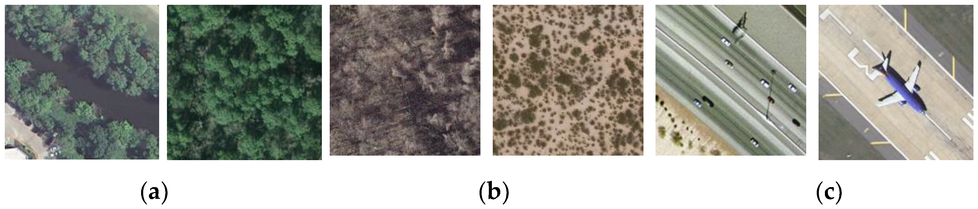
The traditional BOW model uses a universal codebook for all categories without incorporating information of specific scene labels into it [21], which may result in misclassification in categories with similar backgrounds.

(3)

Existing methods incorporating information of labels into BOW model code a testing image with a number of class-specific image representations in each category rather than just one specific representation [21], leading to a large error in mapping universal BOW representation to some inaccurate categories.

In order to solve the first problem, we can use keypoint selection to remove redundant keypoints. Figure 1 shows original extracted SIFT keypoints in (a) and selected keypoints with presented modified keypoint selection method in my text in (b). As we can see, keypoints in (a) are redundant and some of them occur in many other images, after selecting keypoints, we get condensed keypoints that are more helpful for land-use classification.

In the field of keypoint selection or descriptor selection, many experiments have been done to enhance classification performance. Dorko and Schmid [22] introduced a novel method where local descriptors are first divided into several groups using Gaussian Mixture Model (GMM). Then, a Support Vector Machine (SVM) classifier is trained for each group to determine the most discriminative groups. Vidal-Naquet and Ullman [23] proved that using a linear classifier to select informative keypoints delivers better performance. Agarwal and Roth [24] extracts informative parts from images and images can be represented by those parts. Chin et al. [25] proposed the SAMME algorithm to extend the popular AdaBoost algorithm [26] to multiclass problems in order to learn and select the most representative descriptors. However, methods above haven’t focused on the BOW scenario. Lin [27] proposed a two-step iterative keypoint selection method designed for bag-of-word feature, but his initial seed keypoint will have an effect on later keypoint selection results. Therefore, we replace choosing one seed point with a keypoint filter by response value of keypoints.

Traditional BOW model uses a universal codebook for all categories, which may result in misclassification in similar categories as shown in Figure 2. As we can see, these images in (a), (b) and (c) are with similar backgrounds, so their image vocabularies and representations are similar and difficult to distinguish.

Several studies have concentrated on incorporating scene label information into the codebook to improve classification performance. Perronnin [21] creates specifically tuned vocabularies for each image category using the maximum a posteriori (MAP) criterion. Umit [28] proposes a method based on the class-specific codebook derived from Self-Organizing Maps (SOM). Li [29] proposed a method of generating a codebook for each class using piecewise vector quantized approximation (PVQA) on considering the difference between categories. However, these methods delivering better performance in Computer Vision are not suitable for land-use classification of HRIs, since HRIs can provide more complex appearance and spatial arrangements and scene categories in HRIs are largely affected and determined by human and social activities. Therefore, we need to capture the characteristics in each category and we propose a class-specific codebook base on Mutual Information (MI) to evaluate the importance of each vocabulary for each category. The category with the highest MI value in one vocabulary will be assigned to this vocabulary in a class-specific codebook.

Existing methods incorporating information of categories code the testing image with a group of histograms. One histogram of the testing image can be classified by the SVM classifier and the label of class with the largest number of predicting results from SVM will be the final output. The error items of existing methods are illustrated in the left part of Figure 3. Mapping error here means error in mapping universal histograms to class-specific codebook of inaccurate categories, namely the differences between the class-specific histogram of the category and the class-specific histogram of true labels. Mapping error may lead to inaccurately representing the information of scene labels, which may cause misclassification. Therefore, we predict the relatively accurate results of one testing image using a kernel collaborative representation based classification (KCRC) method [30] instead of blind mapping, as shown on the right-hand side of Figure 3.

However, the predicting results of KCRC may still be unreliable since information in HRIs is more detailed in surface features and complexity of scenes than images in Computer Vision. Therefore, we perform classification in two steps to increase classification performance. Firstly, we use KCRC combined with Spatial Pyramid Matching (SPM) to predict two true labels of the testing image instead of just one predicted label. Then we map universal histograms to these two class-specific codebooks. These two class-specific histograms will be respectively put into Support Vector Machine (SVM) [31] for outputting confidence in each label. Then the label with the largest sum of confidence will be the final classification result.

Inspired by the aforementioned work, we incorporate a proposed class-specific codebook into a BOW model for scene-level land-use classification. The main contributions of this paper are summarized below:

(1)

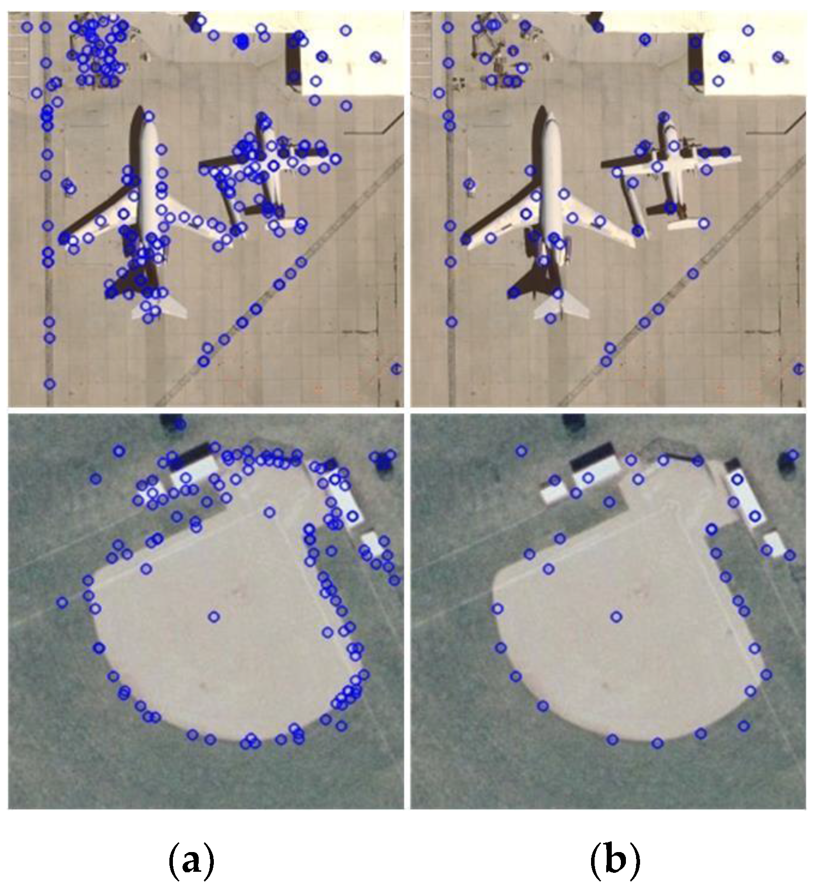
We modify an iterative keypoint selection algorithm with the filter by keypoints’ response values, which enables us to reduce the computational complexity by filtering out indiscriminative keypoints and select representative keypoints for better image representation.

(2)

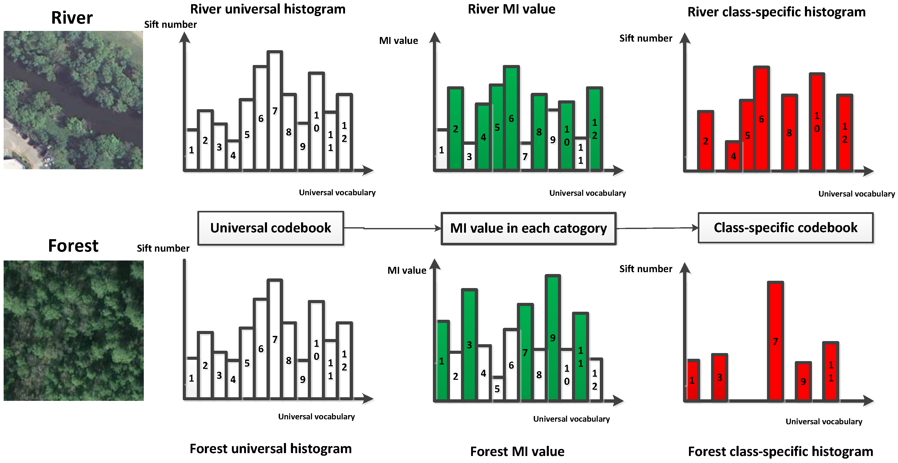
We propose a class-specific codebook designed for HRIs based on feature selection using MI to allocate vocabularies in the universal codebook for each category in order to expand differences between locality-constrained linear coding (LLC) codes of various land use categories.

(3)

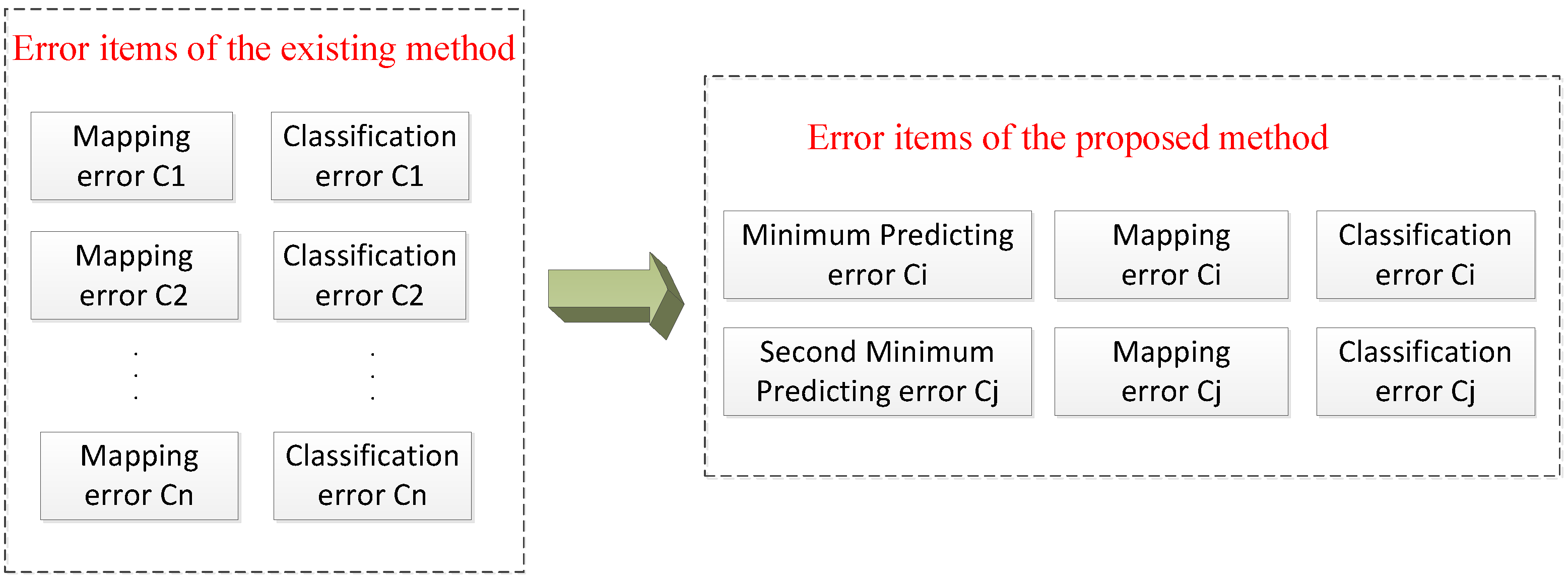
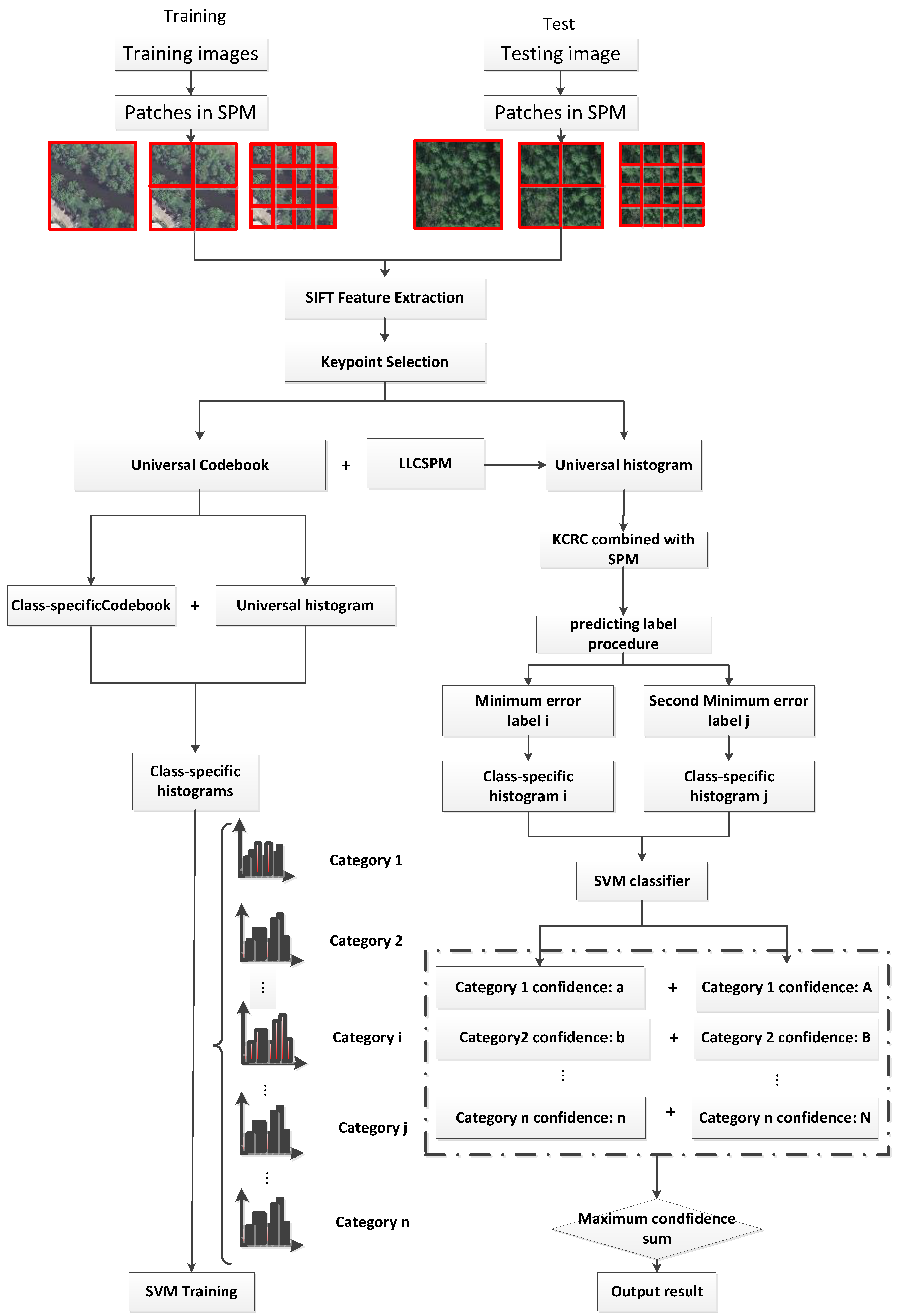
In the testing period, we classify the testing image in two steps. We introduce the KCRC algorithm to obtain two comparatively accurate predicting results of testing samples to make sure the testing sample may be mapped to their unique class-specific codebook and decrease the prediction error by putting these two class-specific histograms respectively into SVM classifiers to output the confidence in each label. The testing image will be assigned to the label with the largest sum of confidence.

The rest of the paper is organized as follows: In Section 2, we describe the overall process of the proposed approach and details of proposed approach. In Section 3, several experiments and results are presented to demonstrate the effectiveness and superiority of the proposed algorithms. In Section 4, a discussion about the proposed method is conducted. Conclusions and suggestions for future work are summarized in Section 5.

2. Materials and Methods

In this section, we present a scene classification method of HRIs based on an improved class-specific codebook as shown in Figure 4, which can be divided into four main steps.

In the first step, dense Scale-Invariant Feature Transform (SIFT) descriptors [18] are extracted from training images in each local patch of Spatial Pyramid Matching(SPM)[32] and are selected using a modified iterative keypoint selection method to remove keypoints that are unhelpful for classification.

In the second step, we use the selected keypoints to generate a universal codebook with “k-means” and get BOW representations in each local patch of SPM by LLC [33].

In the third step, for each category in the training set, we calculate an MI value between each vocabulary and each category to obtain a matrix about MI. Assuming the MI value of one category exceeds that of other categories in a particular vocabulary, then we add this vocabulary to class-specific codebook of that category. Repeating the above procedure, we finally get a unique class-specific codebook in each category.

Finally, we perform classification in two steps on testing datasets. Firstly, we use a KCRC combined with the SPM method to predict two true labels of testing sample and the testing sample are mapped to these two class-specific codebooks. Then we represent the testing image with two class-specific histograms. These two class-specific histograms will be respectively put into a Support Vector Machine (SVM) to compute the confidence in each label. Then the label with the largest sum of confidence will be the final classification result.

Details of those specific principles and implementation processes are provided in the subsequent sub sections.

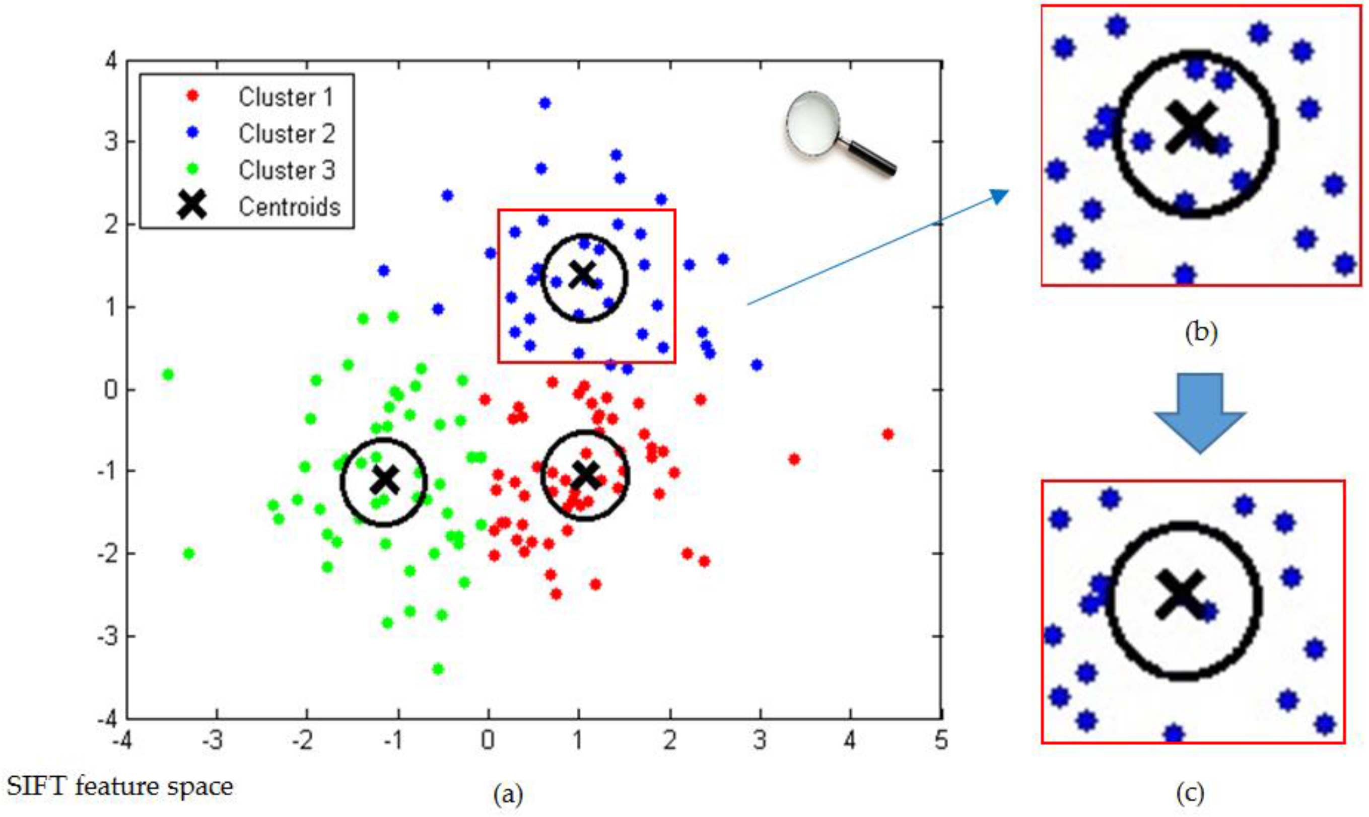
2.1. Iterative Keypoint Selection with the Filter by Keypoints’ Response Values

The central idea of iterative keypoint selection method [27] is illustrated in Figure 5. In one iteration, we identify the discriminative descriptors and filter out unrepresentative ones with a distance measure since keypoints with similar descriptors appear to be close. The iteration repeats until no unrepresentative descriptors are filtered out.

The key problem of iterative keypoint selection is to how to choose discriminative keypoints. Lin randomly chose one keypoint as the initial keypoint. Thus, the location of the initial keypoint will have an effect on the selection results.

In order to solve the problem of initial keypoint selection, we use response value with neighboring keypoints to reflect the saliency of keypoints. We remove keypoints with lower contrast than a threshold $\theta$ according to Equation (1).

$$D(\stackrel{\wedge }{X})=D+\frac{1}{2}\frac{\partial D^T}{\partial X}\frac{{\partial }^2{D}^{-1}}{\partial X^2}\frac{\partial D}{\partial X}<\theta$$

(1)

where D is the value of Difference of Gaussian (DOG) function [6] in the location of keypoints and $X=(x,y,\sigma )$ is the offset of keypoints.

Filter of response value can not only avoid the problem of initial keypoint selection but also remove some unreliable keypoints which are not different from neighboring keypoints since we just need a critical keypoint for image representation. This step can help to offer discriminative results for the later iterative keypoint selection.

Then filtered keypoints are clustered using “k-means” in the SIFT feature space. Keypoints closest to the cluster center are regarded as representative keypoints. Keypoints whose Euclidean distance in SIFT feature space are within a threshold T of those representative keypoints will be removed. This is the first iteration of selection.

The selection results of the first iteration will be used as the initial keypoints in the second iteration and the procedure will be the same as in the first iteration. The iteration repeats until no keypoints will be filtered out or remaining keypoints are inadequate to be clustered.

The proposed keypoint selection can not only improve computational efficiency but also remove keypoints that are unhelpful for classification to enhance classification performance in HRIs land-use classification.

2.2. LLC Coding

Traditional SPM solves the following constrained least square fitting problem using Vector Quantization (VQ) coding [32] in Equation (2):

$$\begin{array}{l}\arg \underset{C}{\min }{\displaystyle \sum _{i=1}^C{\Vert x_i-B{c}_i\Vert }^2}\\ s.t.{\Vert c_i\Vert }_{l^0}=1,{\Vert c_i\Vert }_{l^1}=1,c_i\ge 0,\forall i\end{array}$$

(2)

where an image is represented by a set of extracted dense SIFT descriptors X, namely $X=\left[x_1,x_2,\dots ,x_C\right]\in R^{D\times C}$, $B=[b_1,b_2,\dots ,b_M]\in R^{D\times M}$ is a codebook containing m vocabularies and $C=[c_1,c_2,\dots ,c_C]$ is the VQ codes calculated from X.

However, VQ coding may lead to vector quantization error due to the hard-assignment strategy. In order to solve this problem, the restrictive cardinality constraint ${\Vert c_i\Vert }_{l^0}=1$ in Equation (3) can be relaxed by using a sparsity regularization term in ScSPM [34]. Moreover, it is a standard sparse coding (SC) problem how to code each SIFT descriptor $x_i$ with a soft-assignment strategy. The SC problem can be solved in Equation (4):

$$\arg \underset{c}{\min }{\displaystyle \sum _{i=1}^C{\Vert x_i-B{c}_i\Vert }^2}+\lambda {\Vert c_i\Vert }_{l^1}$$

(3)

As suggested by J. Wang [31], sparsity is not as essential as locality since locality must result in sparsity but not vice versa. The LLC coding can be solved in Equation (4):

$$\begin{array}{l}\underset{c}{\min }{\displaystyle \sum _{i=1}^C{\Vert x_i-B{c}_i\Vert }^2+\lambda {\Vert d_i\odot c_i\Vert }^2}\\ s.t.1^T{c}_i=1,\forall i\end{array}$$

(4)

where $\odot$ means multiplication of each element in matrix $d_i$ and $c_i$, and $d_i\in R^M$ is the locality adaptor assigning distinctive freedom to each vocabulary in codebook according to its similarity to the SIFT descriptor $x_i$ in Equation (5).

$$d_i=\exp (\frac{dist(x_i,B)}{\sigma })$$

(5)

where $dist(x_i,B)={[dist(x_i,b_1),\dots ,dist(x_i,b_M)]}^T$ and $dist(x_i,b_j)$ is the Euclidean distance between the SIFT descriptor $x_i$ and vocabulary $b_j$, σ is used for adjusting the weight decay speed for the locality adaptor. Then the max-pooling strategy is applied to the coding results C to get the final LLC coding.

For each local patch extracted by SPM, we get the LLCSPM coding with Equation (6). Then we fuse the LLC coding with the weight in SPM to form a longer LLCSPM coding to represent the image.

$$LLC=\left[\frac{1}{4}LL{C}_0,\frac{1}{4}LL{C}_1^1,\dots ,\frac{1}{4}LL{C}_1^4,\frac{1}{2}LL{C}_2^1,\dots ,\frac{1}{2}LL{C}_2^{16}\right]$$

(6)

where $LL{C}_i^j$ represents the LLC code in the $j$th patch on the i-th level of SPM.

LLC combined with SPM not only incorporates spatial information into BOW model but also demonstrates the lowest vector quantization error.

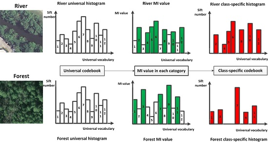
2.3. Generation of Class-Specific Codebook Using MI

The class-specific codebook is obtained through the vocabulary selection from the universal codebook for each category using class-specific data in training set. The class-specific codebook has two interesting properties [21]. It needs fewer training samples to estimate parameters of the specific category since during vocabulary selection we have made some assumptions on the a priori location of parameters in the whole parameter space. Moreover, the class-specific codebook maintains some correspondence with the universal codebook since it is derived from the universal codebook.

After obtaining the universal codebook and universal histogram with the above methods, we can obtain a class-specific codebook and class-specific histogram as shown in Figure 6. Assume that we need to generate a class-specific codebook in two categories, forest and river. As we can see in Figure 6, if the number of visual words is equal to 2, the vocabularies in the universal codebook are assigned to only one of the two categories respectively according to their MI value. If the MI value of forest is above that of river, then this vocabulary marked with the green color will be assigned to forest and vice versa. Each vocabulary can only belong to one specific category. Finally, we will get a class-specific codebook and the number of red bars is the vocabulary that belongs to the class-specific codebook. The red bar represents the class-specific histogram derived from the universal histogram.

The green bar means the MI value of this vocabulary tops that of the same vocabulary in all other vocabularies and the red bar means the class-specific histogram derived from the universal histogram.

As we can see, the universal histograms of river and forest are similar, which may result in misclassification. However, we chose the most representative vocabulary from the universal codebook for each category and only one vocabulary can exist in just one class-specific codebook. That is to say, vocabularies best representing this class-specific codebook will exist in this class-specific codebook. Thus, the class-specific codebook can better reflect the information of this category. Mapping the universal histogram to the class-specific codebook means value will exist in vocabularies that belong to this class-specific codebook. Values in other vocabularies of this codebook will be 0. The dimension of universal histograms is the same as that of class-specific histograms, but the class-specific histogram is more discriminative since it reflects information belonging to its own labels rather than information about the whole image. Details of the generation of the class-specific codebook will be illustrated as follows.

The MI value between each vocabulary and each category reflects contributions of each vocabulary to each category. MI value can be calculated as Equation (7).

$$MI(b_i|c_j)=\log (\frac{P(b_i|c_j)}{P(b_i)})$$

(7)

where $b_i$ is the i-th vocabulary in the universal codebook and $c_j$ is the j-th category in scene labels. $P(b_i|c_j)$ reflects the possibility that $b_i$ exists in training samples of $c_j$ and $P(b_i)$ is the possibility of $b_i$ existing in the training set.

As illustrated above, we calculate MI values between each vocabulary and each category to obtain a matrix concerning MI values as Equation (8) shows:

$$\left[\begin{array}{ccc}MI(b_1|c_1),& MI(b_1|c_2),\dots ,& MI(b_1|c_n)\\ MI(b_2|c_1),& MI(b_2|c_2),\dots ,& MI(b_2|c_n)\\ ⋮\hfill & ⋮& ⋮\\ MI(b_M|c_1),& MI(b_M|c_2),\dots ,& MI(b_M|c_n)\end{array}\right]$$

(8)

For each row in the Equation (8), we can obtain a maximum, such as $MI(b_i|c_j)$. Then we add $b_i$ to the class-specific codebook of $c_j$. After traversal of all vocabularies in the universal codebook, we will finally get the class-specific codebook in each category.

2.4. KCRC Combined with SPMPpredicting Method and Two-Step Classification

As shown in Figure 3, in methods related to the class-specific codebook, bag-of-features are usually mapped to each category to get histograms in each category for classification. If bag-of-features are mapped to inappropriate class-specific codebooks, the predicting results might be incorrect and this class-specific histogram will be useless for classification. In order to overcome the limitations, we present a KCRC combined with the SPM algorithm to obtain two accurate predicting outcomes for the testing sample. Details of KCRC method are illustrated as follows.

Assuming $X_i=[x_{i,1},x_{i,2},\dots ,x_{i,n_i}]\in R^{21\times M\times n_i}$ is the LLC codes combined with SPM in the training sample of i-th class, where $x_{i,j}(j=1,2,\dots ,n_i)$ is a vector with a dimension of $21\times M$, namely 3 levels of spatial pyramid, from the j-th training samples in the i-th class. $y_0\in R^{21\times M}$ is the LLC codes of a testing sample and training samples are $X=\left[X_1,X_2,\dots ,X_C\right]$ with C categories. Then the testing sample can be represented by a linear combination of training samples $y_0=w_{0}X$, where $w_0={[0,\dots ,0,w_{i,1},w_{i,2},\dots ,w_{i,n_i},0,\mathrm{..},0]}^T$.

KCRC method can effectively discover nonlinear structures such as changes of illumination, spectral noise [35] and large attitude by mapping the samples into a higher dimensional space and operating traditional CRC [36] method in this high-dimensional space. Denote $\mathrm{\Phi }=[\varphi (x_{1,1}),\varphi (x_{1,2}),\dots ,\varphi (x_{c,n_c})]$ as the mapped samples from the original feature space to a high-dimensional space and we employ the Gaussian radial basis function (RBF) kernel $k(x,y)={\exp }^{-\sigma {\Vert x-y\Vert }_2^2}$ for better fitting the SVM RBF kernel classifier.

The KCRC combined with the SPM Algorithm can be illustrated as follows：

LLC codes combined with SPM are calculated for each training sample and the testing sample. $y_0$ is the testing sample and X are the training samples.

The objective function of the KCRC algorithm $w=\arg \min {\Vert \mathrm{\Phi }(y_0)-\mathrm{\Phi }w\Vert }_2^2+\lambda {\Vert w\Vert }_2^2$ can be directly solved in Equation (9)

$$w={({\mathrm{\Phi }}^T\mathrm{\Phi }+\lambda I)}^{-1}{\mathrm{\Phi }}^T\varphi (y_0)$$

(9)

where

$$\begin{array}{c}{\mathrm{\Phi }}^T\mathrm{\Phi }={[\varphi (x_{1,1}),\varphi (x_{1,2}),\dots ,\varphi (x_{c,n_c})]}^T\cdot \left[\varphi (x_{1,1}),\varphi (x_{1,2}),\dots ,\varphi (x_{c,n_c})\right]\\ =\left[\begin{array}{cccc}k(x_{1,1},x_{1,1})& k(x_{1,1},x_{1,2})& \cdots & k(x_{1,1},x_{c,n_c})\\ k(x_{1,2},x_{1,1})& k(x_{1,2},x_{1,2})& \cdots & k(x_{1,2},x_{c,n_c})\\ ⋮\hfill & ⋮& & \ddots \hfill \\ k(x_{c,n_c},x_{1,1})& k(x_{c,n_c},x_{1,2})& \cdots & k(x_{c,n_c},x_{c,n_c})\end{array}\right]\end{array}$$

(10)

and

$${\mathrm{\Phi }}^T\varphi (y_0)=\left[\varphi (x_{1,1}),\varphi (x_{1,2}),\dots ,\varphi (x_{c,n_c})\right]\cdot \varphi (y_0)=\left[\begin{array}{l}k(x_{1,1},y_0)\\ k(x_{1,2},y_0)\\ ⋮\\ k(x_{c,n_c},y_0)\end{array}\right]$$

(11)

The regularized residuals $r_i(y_0)$ in each category can be calculated by Equation (12)

$$r_i(y_0)=\frac{{\Vert \varphi (y_0)-{\mathrm{\Phi }}_i{w}_i\Vert }_2}{{\Vert w_i\Vert }_2}fori=1,\dots ,c$$

(12)

where

$$\begin{array}{l}{\Vert \varphi (y_0)-{\mathrm{\Phi }}_i{w}_i\Vert }_2=\sqrt{{(\varphi (y_0)-{\mathrm{\Phi }}_i{w}_i)}^T(\varphi (y_0)-{\mathrm{\Phi }}_i{w}_i)}\\ =\sqrt{k(y_0,y_0)+{w_i}^T{{\mathrm{\Phi }}_i}^T{\mathrm{\Phi }}_i{w}_i-2{(\varphi (y_0))}^T{\mathrm{\Phi }}_i{w}_i}\end{array}$$

(13)

$$\begin{array}{c}{{\mathrm{\Phi }}_i}^T{\mathrm{\Phi }}_i={[\varphi (x_{i,1}),\varphi (x_{i,2}),\dots ,\varphi (x_{i,n_i})]}^T\cdot \left[\varphi (x_{i,1}),\varphi (x_{i,2}),\dots ,\varphi (x_{i,n_i})\right]\\ =\left[\begin{array}{ccccc}k(x_{i,1},x_{i,1})& k(x_{i,1},x_{i,2})& \cdots & k(x_{i,1},x_{i,n_i})& \\ k(x_{i,2},x_{i,1})& k(x_{i,2},x_{i,2})& \cdots & k(x_{i,2},x_{i,n_i})& \\ ⋮\hfill & ⋮& & \ddots \hfill & \dots \\ k(x_{i,n_i},x_{i,1})& k(x_{i,n_i},x_{i,2})& \cdots & k(x_{i,n_i},x_{i,n_i})& \end{array}\right]\end{array}$$

(14)

and

$$\varphi {(y_0)}^T{\mathrm{\Phi }}_i=\left[k(y_0,x_{i,1}),k(y_0,x_{i,2}),\dots ,k(y_0,x_{i.n_i})\right]$$

(15)

The predicted label will be two with the lowest and the second lowest residuals.

$$y=\arg \underset{i}{\min } r_i(y_0)\cup y=\arg \underset{i,i\ne y}{\min }{r}_i(y_0)$$

(16)

Since the KCRC method may produce inaccurate predicted labels, we use two labels rather than one predicted label to avoid misclassification with the most similar category. Therefore, we classify the testing image in two steps. The procedure of first classification is shown from Equations (9) to (16) using KCRC above.

Then, during the period of the second classification, LLC codes in each testing sample will be mapped to the class-specific codebook of both predicted labels to generate two class-specific histograms. Each class-specific histogram will be respectively put into SVM classifiers to output the confidence of each label. The label with the largest sum of confidence will be the final result.

3. Experiments and Results

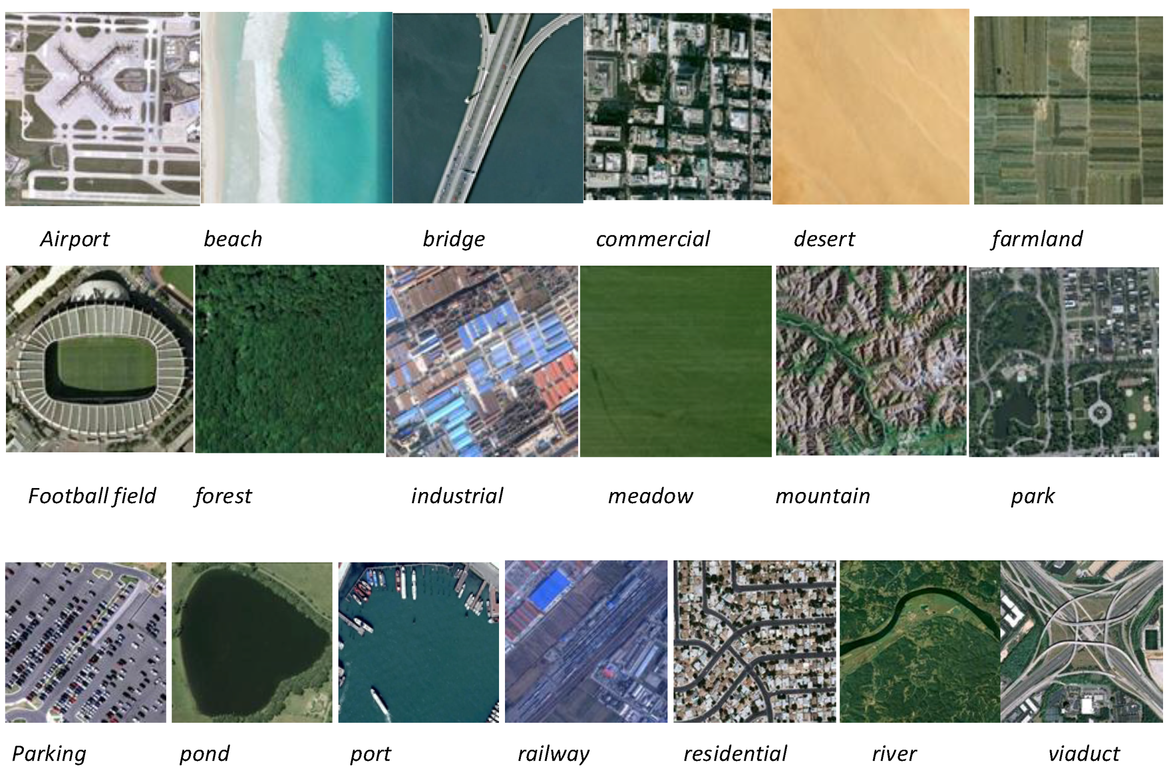
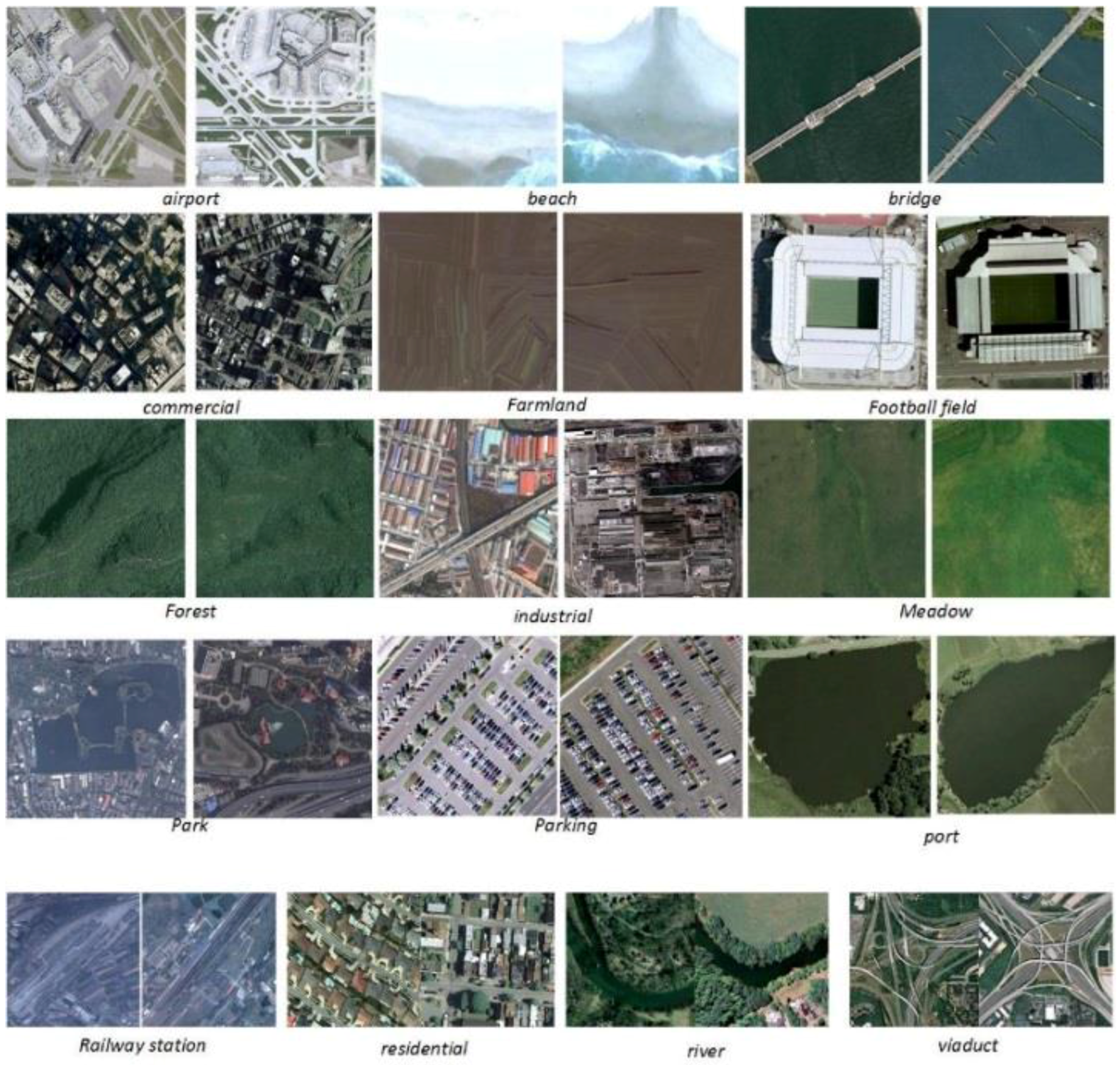
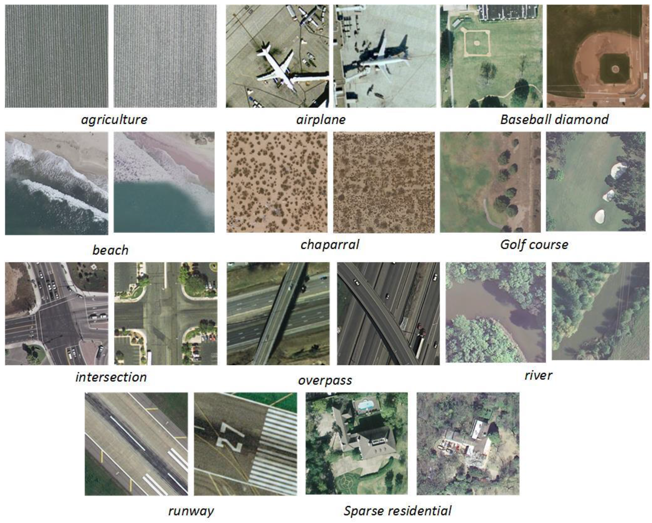
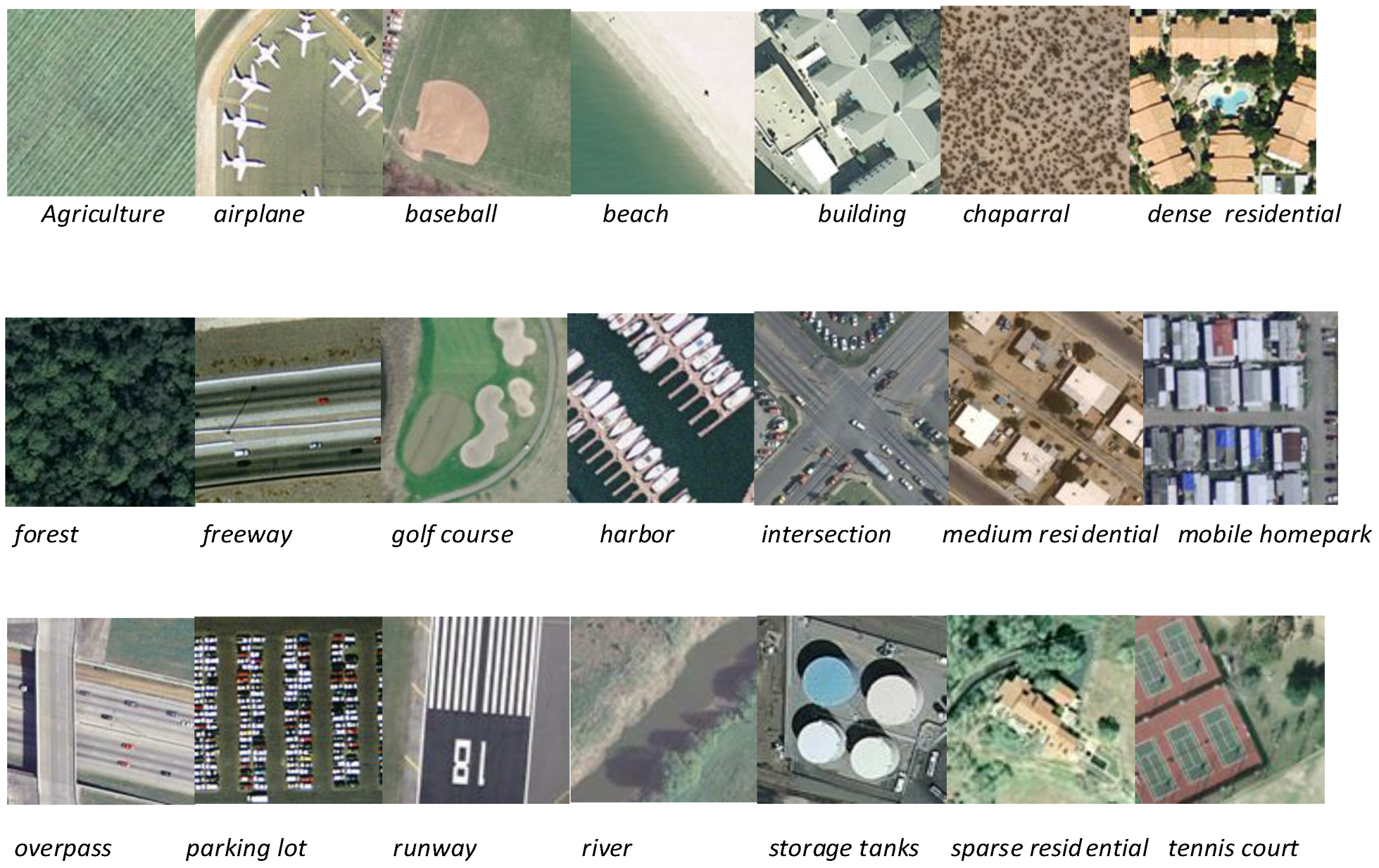
3.1. Experimental Data and Setup

The first dataset is a ground truth dataset consisting of 21 scene categories [18] named University of California, Merced (UC_MERCED) dataset. This dataset was manually extracted from aerial orthoimagery and downloaded from the United States Geological Survey (USGS) National Map. The 21 classes include agricultural, airplane, baseball diamond, beach, buildings, chaparral, dense residential, forest, freeway, golf course, harbor, intersection, medium density residential, mobile home park, overpass, parking lot, river, runway, sparse residential, storage tanks, and tennis courts. Each category contains 100 images of size 256 × 256 pixels with a resolution of 30 cm in the RGB color space. Sample images in each category of this dataset are shown in Figure 7.

The second dataset used in our experiments is the High-resolution Satellite Scene Dataset in Wuhan University (WHU-RS) satellite scene dataset [37]. This dataset is a new publicly available dataset wherein all the images are collected from Google Earth (Google Inc. Mountain View, CA, USA). It consists of high resolution satellite scenes of 19 categories including airport, beach, bridge, commercial, desert, farmland, football field, forest, industrial, meadow, mountain, park, parking, pond, port, railway station, residential, river and viaduct. There are 50 images of size 600 × 600 pixels for each class. Sample images of each class in this dataset are shown in Figure 8.

In this paper, we randomly choose 20 images from each class for training and the rest for testing in the WHU-RS dataset and 50 images for training in the UC_MERCED dataset. In order to measure the performance of the proposed algorithm, we use four comparison approaches in different experiments, namely, the BOVW without keypoint selection [20], BOVW with the proposed keypoint selection method, existing methods incorporating the traditional class-specific codebook [21] and existing methods without the class-specific codebook. Dense SIFT features are extracted for each image and a three-level pyramid was applied for LLCSPM. Contrast experiments were made on thresholds of response value, distance threshold and different number of clusters to get the optimal keypoint selection parameter settings. We used the public LIBSVM package [38] and the classical radial basis function (RBF) kernel [39] was selected for multiclass classification with the same SVM parameters. For RBF Kernels, the penalty coefficient C and the kernel parameter $\gamma$ were selected using a grid search by cross validation. The criterion for searching C and $\gamma$ is as follows:

$$C\in \left\{2^{-5},2^{-4},\dots ,2^4,2^5\right\},\gamma \in \left\{2^{-5},2^{-4},\dots ,2^4,2^5\right\}$$

The optimal parameter settings we finally get is $C=4,\gamma =0.5$. The experiment is run 5 times and the final accuracy will be average classification accuracy. The computer environment is based on Intel Core i7-3770 with 8GB of RAM.

3.2. Results of the Keypoint Selection Algorithm

It is well-known that the state-of-the-art keypoint selection algorithms are IB3 [40], DROP3 [41], ICF [42] and Iterative Keypoint Selection (IKS) [27], as mentioned in Section 2.1. Since IKS is an efficient algorithm in keypoint selection, it is used for comparison with the modified keypoint selection algorithm in both datasets to demonstrate the superiority of the modified method.

Table 1. Number of average remaining keypoints in our method and IKS and their standard deviation.

Method	WHU-RS Dataset	UC_MERCED Dataset
BOW without keypoint selection	1,513,532 ± 21,888	939,657 ± 17,339
Filter with response value (First step)	862,745 ± 16,411	554,310 ± 13,517
Proposed Keypoint Selection Method	635,497 ± 14,227	403,857 ± 11,259
IKS	575,168 ± 29,110	356,952 ± 10,403

shows the average number of Remaining keypoints by the first step and both steps of modified keypoint selection and baseline method IKS along with their standard deviation. As we can see, there is a large number of keypoints that must be selected from the training set, 1,513,532 and 939,657 keypoints over WHU-RS and UC_MERCED land-use classification, respectively. IKS obtains a slightly higher selection rate in UC_MERCED and WHU-RS classification.

However, as can be seen in

Table 2. Comparison in average computational time for vector quantization and classification accuracy along with their standard deviation for both datasets.

	Method	BOW without Keypoint Selection	Filter with Response Value	Proposed Keypoint Selection Method	IKS
Dataset
UC_MER CED	time	252 ± 1.9 min	222 ± 2.8 min	135 ± 2.5 min	478 ± 3.3 min
	accuracy	0.715 ± 0.0036	0.736 ± 0.0033	0.7780 ± 0.0028	0.721 ± 0.0045
WHU-RS	time	387 ± 4.5 min	316 ± 3.3 min	221 ± 2.9 min	630 ± 5.1min
	accuracy	0.686 ± 0.0029	0.698 ± 0.0032	0.754 ± 0.0036	0.695 ± 0.0033

, a lot less time is needed to complete the vector quantization and the highest classification is achieved in both datasets with modified keypoint selection method since the algorithm removes indiscriminative keypoints. The first step, the filtering of keypoints with response values, obtains less computational time and a little bit higher classification accuracy. Although a large number of keypoints can be selected by IKS, IKS requires a lot more computational time with a little increase in classification accuracy.

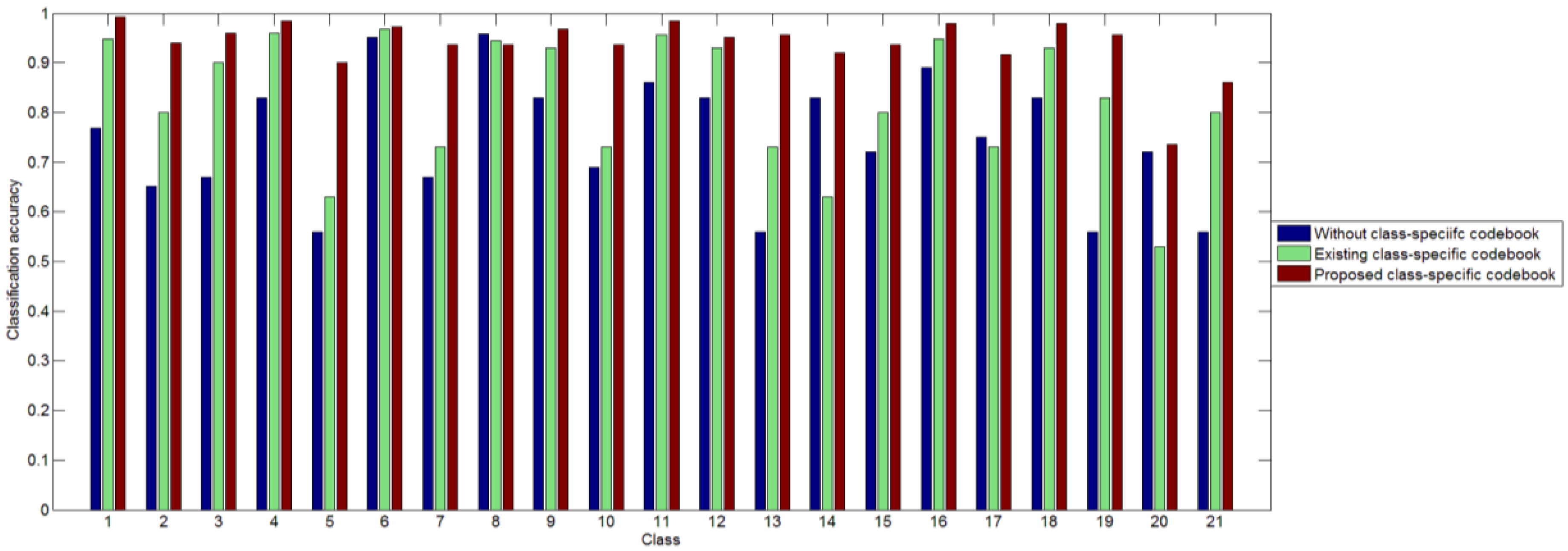
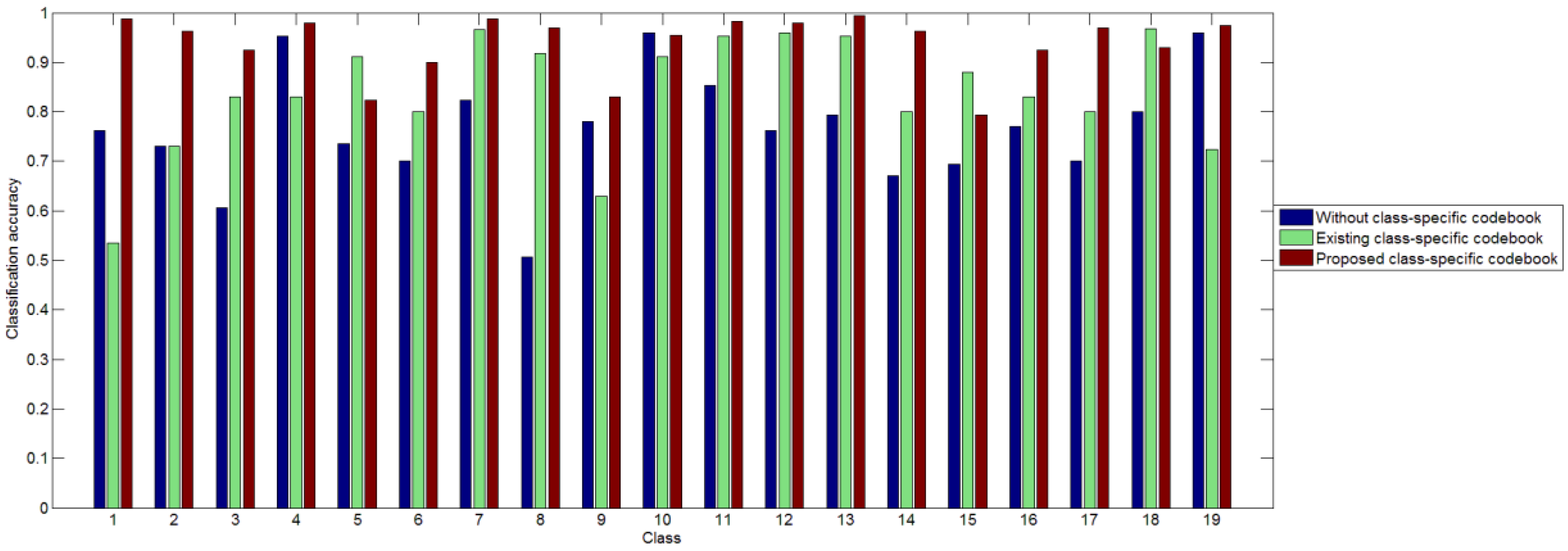
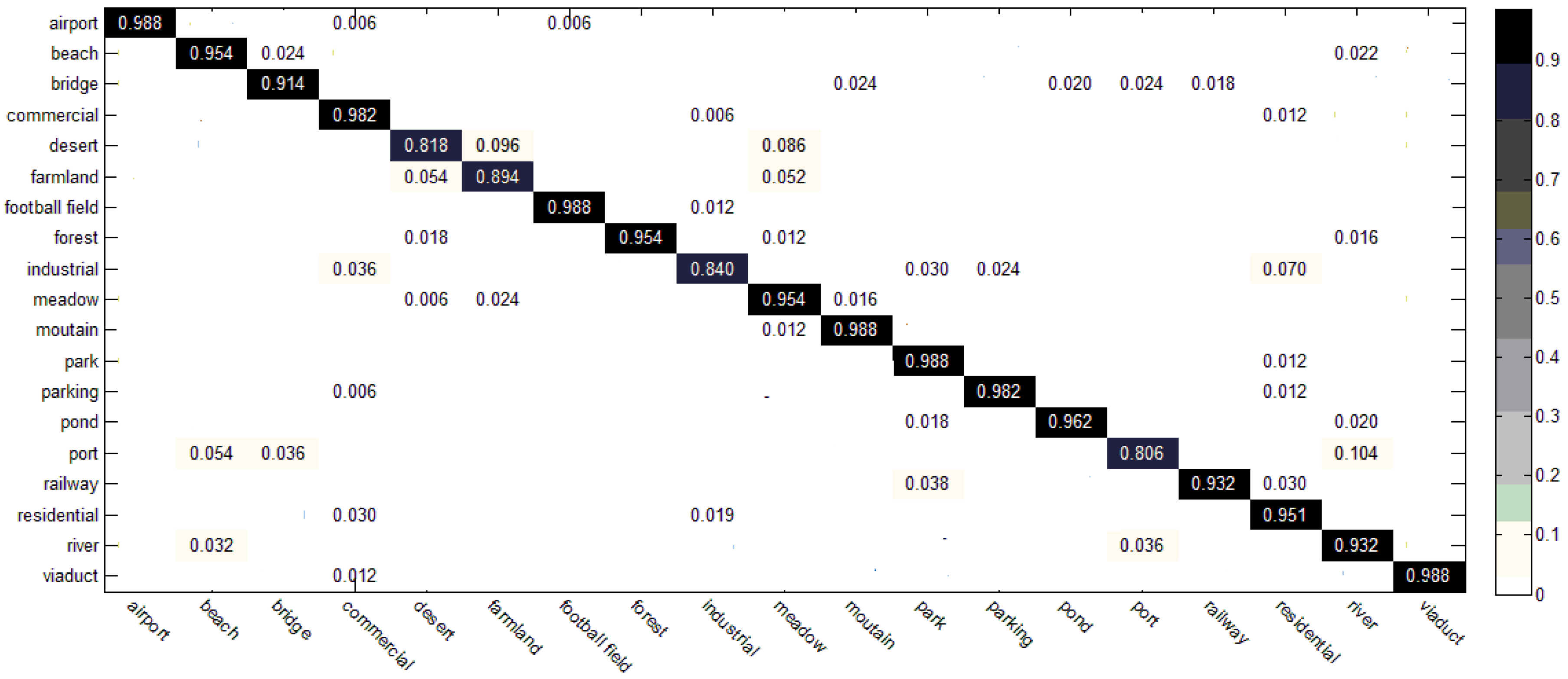
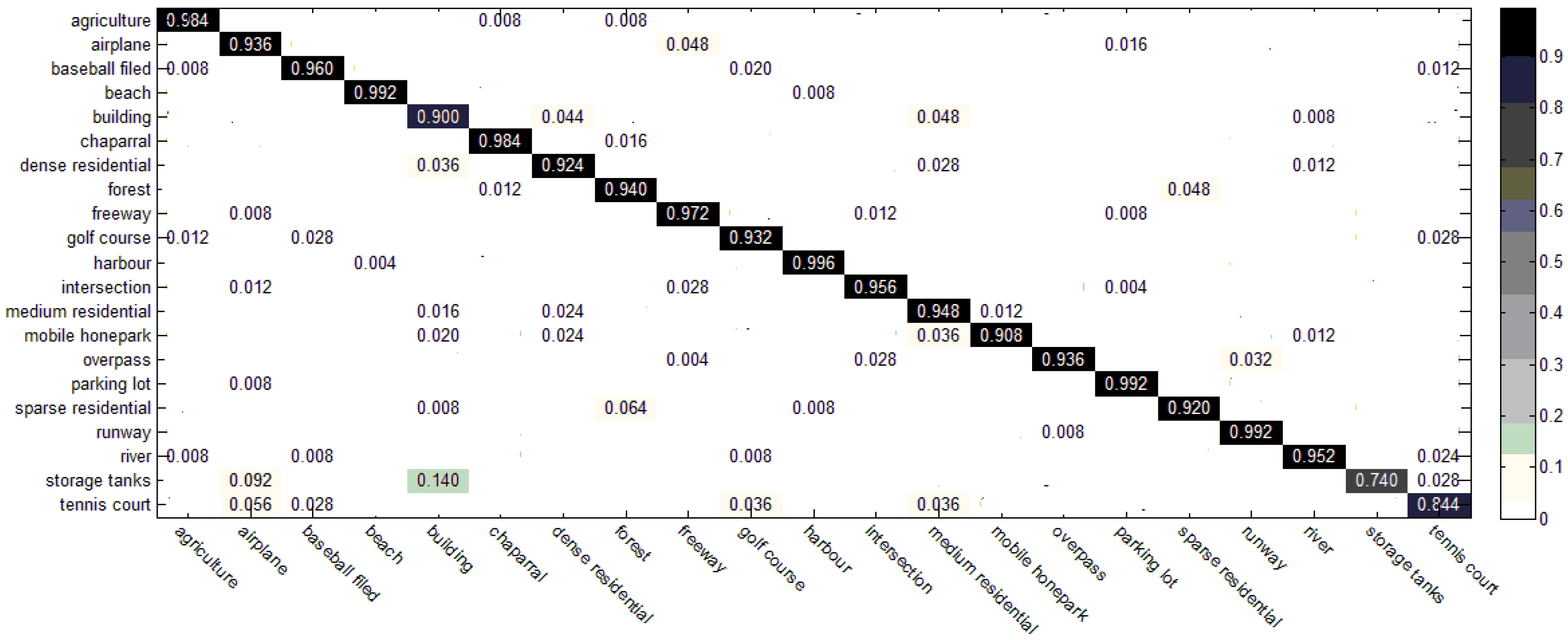
3.3. Results of the Two-Step Classification Method

KCRC has demonstrated promising performance in classification, but it still needs to be improved. Figure 9 and Figure 10 display the testing samples in respectively two datasets which are predicted incorrectly with KCRC combined with SPM method but classified correctly in our two-step classification approach.

As we can see in Figure 9, in most testing samples that KCRC has misclassified, the category may be misclassified into categories of their backgrounds. Therefore, our proposed algorithm is more robust for those images with backgrounds of similar color or texture such as port surrounded by grass, river surrounded by forests and bridge on the river and so on. Similarly, in Figure 10, we can see buildings with forests, fields with grass on and also rivers surrounded by forests.

Table 3. Classification results of both datasets with KCRC and our proposed algorithm.

Different Conditions	UC_MERCED Dataset	WHU-RS Dataset
Total testing samples	1050	570
KCRC right	0.843 ± 0.0036	0.851 ± 0.0033
KCRC wrong but proposed right	0.116 ± 0.0029	0.109 ± 0.0028
KCRC right but proposed wrong	0.019 ± 0.0013	0.019 ± 0.0015

shows the average classification accuracy of both datasets and their standard deviation under conditions of KCRC and two-step classification. As we can see, KCRC shows excellent classification performance with a classification accuracy of about 85% but it stills misclassifies about 15% of the testing samples. As shown in Table 3, two-step classification has a positive effect on classification results. In some testing samples where KCRC has misclassified, about 11% of testing samples, our proposed algorithm demonstrates better performance although nearly 1.9% of testing samples that KCRC has correctly classified are misclassified with our two-step classification method.

Figure 11 displays the classification accuracy in each category with three different contrast methods mentioned in Section 3.1 using the UC_MERCED land-use dataset. As can be seen, the proposed algorithm outperforms the other two methods in almost all categories by at least 3% and BOW incorporating traditional class-specific codebook performs the second best followed by methods without a class-specific codebook. However, in some categories, such as forest and storage tanks, our proposed algorithm demonstrates a slightly lower classification accuracy than the traditional BOW model incorporating the class-specific codebook.

Similarly, as we can see in Figure 12, the proposed approach yields the highest classification accuracy in most categories followed by the BOW model incorporating traditional class-specific codebook. However, in some categories including desert, meadow, port and river, the two-step classification method demonstrates a slightly lower classification accuracy.

Figure 13 further shows the confusion matrix for the two-step classification algorithm using WHU-RS land-use dataset. As we can see, almost all categories perform well with an accuracy close to 1 except for desert, industrial and port with an accuracy below 0.85. Desert categories are confused with farmland, meadow scenes and industrial scenes are confused with commercial, park and residential scenes and port scenes are confused with beach, bridge and river scenes.. These three categories are misclassified into more than one category.

Similarly, Figure 14 shows the confusion matrix using UC_MERCED land-use classification with the proposed method. As can be seen, only classification accuracy in tennis court, storage tanks and building category are below 0.9. In this dataset, these three categories are also misclassified into several categories. For example, buildings are confused with dense and medium residential areas and storage tanks are misclassified into airplanes, buildings and tennis courts.

3.4. Comparison with the State-of-the-Art

In order to prove the superiority of the proposed improved class-specific codebook, we compare its classification performance on both datasets with the state-of-the-art performance reported in the literature such as LDA [11], Improved Fisher Kernel [43], Vector of Locally Aggregated Descriptors (VLAD) [44] and promising GoogLeNet [17] under similar experimental setup.

As shown in

Table 4. Compare classification accuracy of proposed method with state of art methods.

	Method	LDA	IFK	VLAD	GoogLe Net	Proposed Method
Dataset
UC_MERCED		0.642 ± 0.0019	0.826 ± 0.0028	0.778 ± 0.0036	0.925 ± 0.0049	0.938 ± 0.0058
WHU-RS		0.708 ± 0.0015	0.835 ± 0.0025	0.805 ± 0.0033	0.923 ± 0.0045	0.937 ± 0.0057

, the proposed method achieves about 1.2% higher in classification accuracy, as compared with the best performance in GoogLeNet, which is famous as a deep learning method. Compared with other state-of-the-art methods except the high-level GoogLeNet method, our proposed method achieves more than 12% higher classification accuracy.

The superior performance, as compared with the current state-of-the-art results on both datasets, demonstrates the effectiveness of the proposed method for HRIs scene-level land-use classification.

4. Discussion

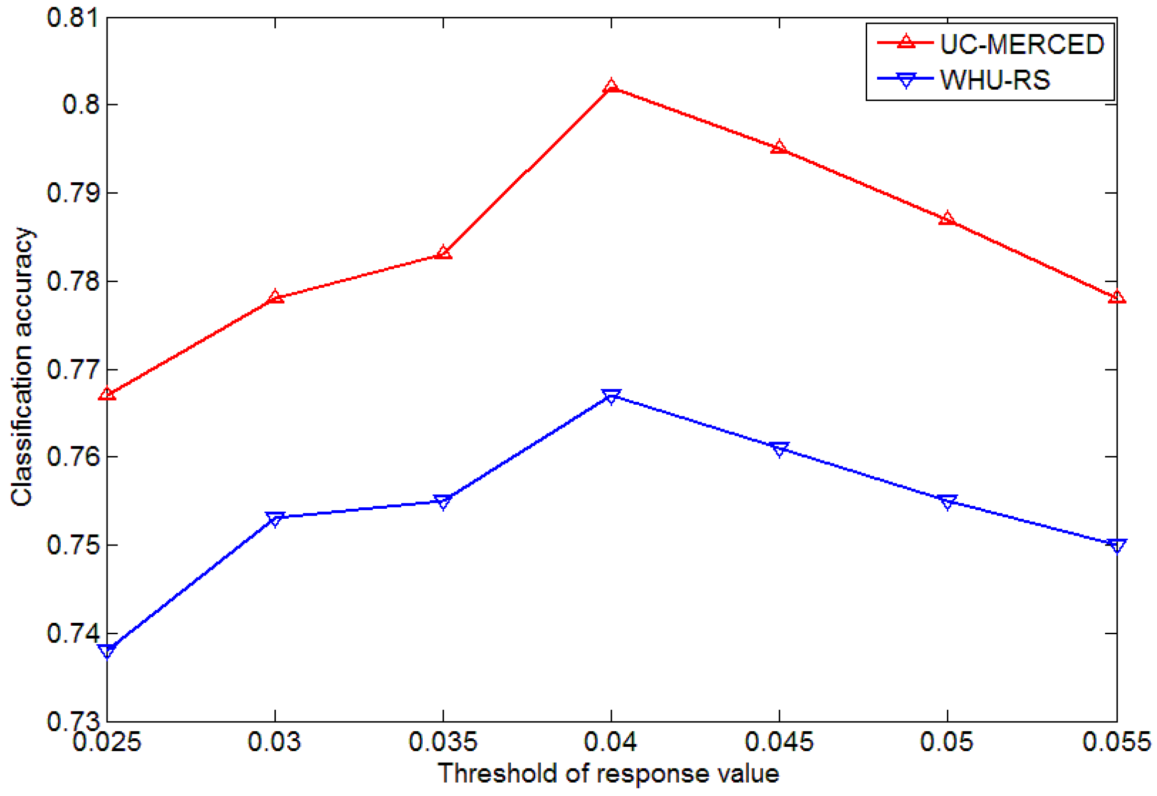
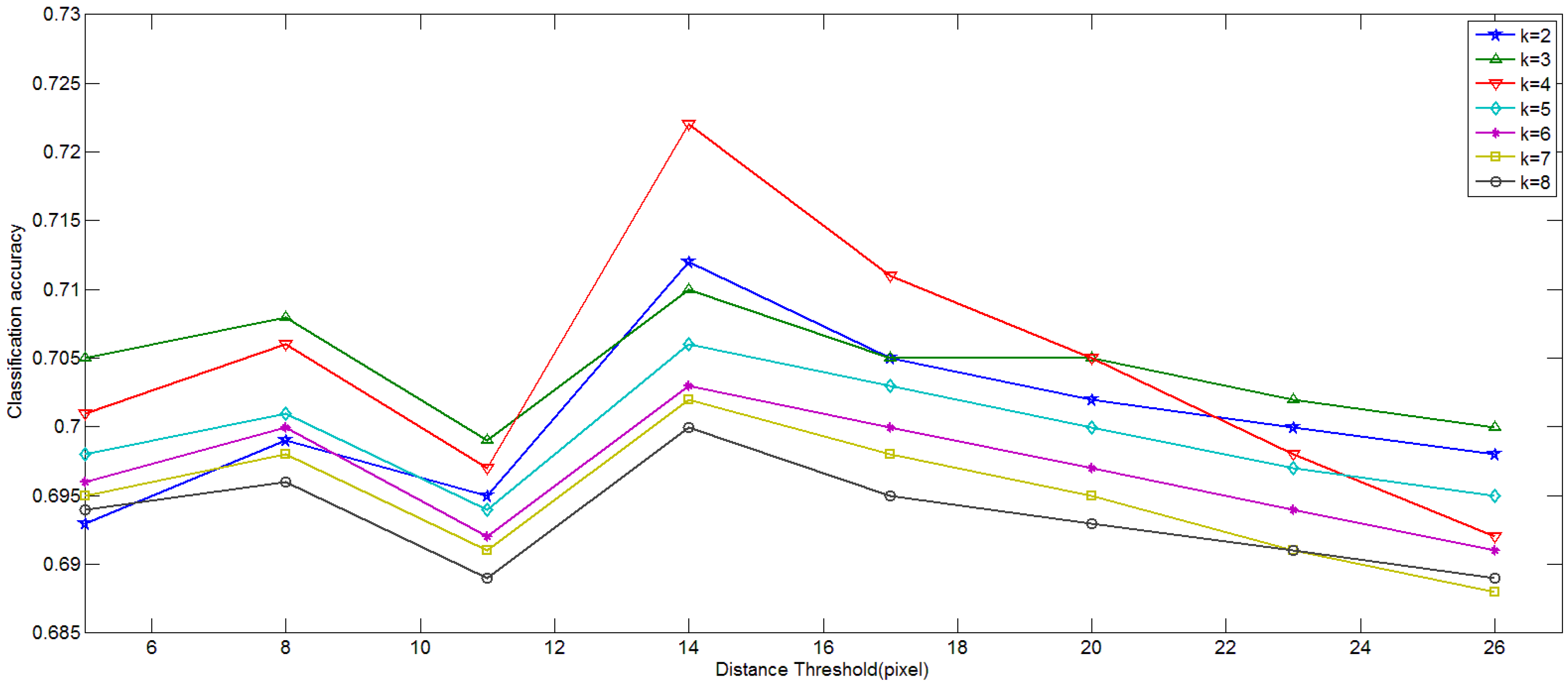
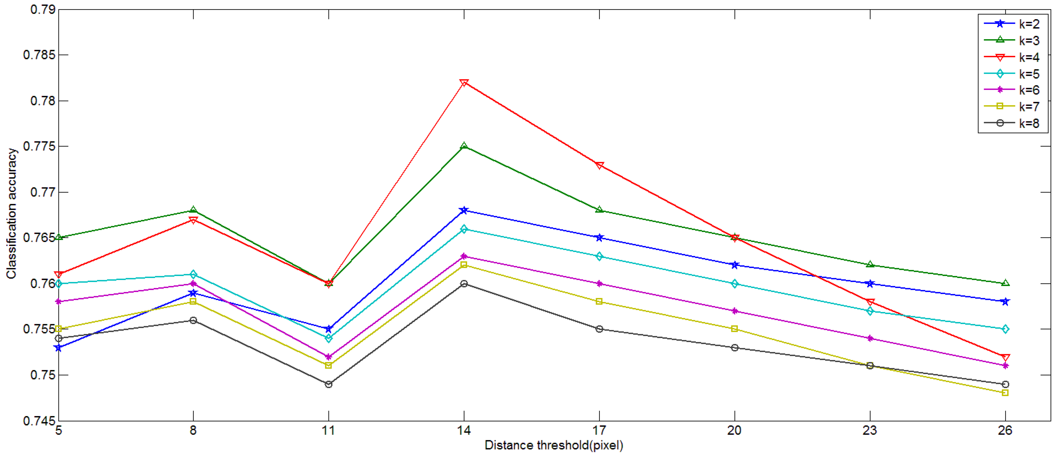
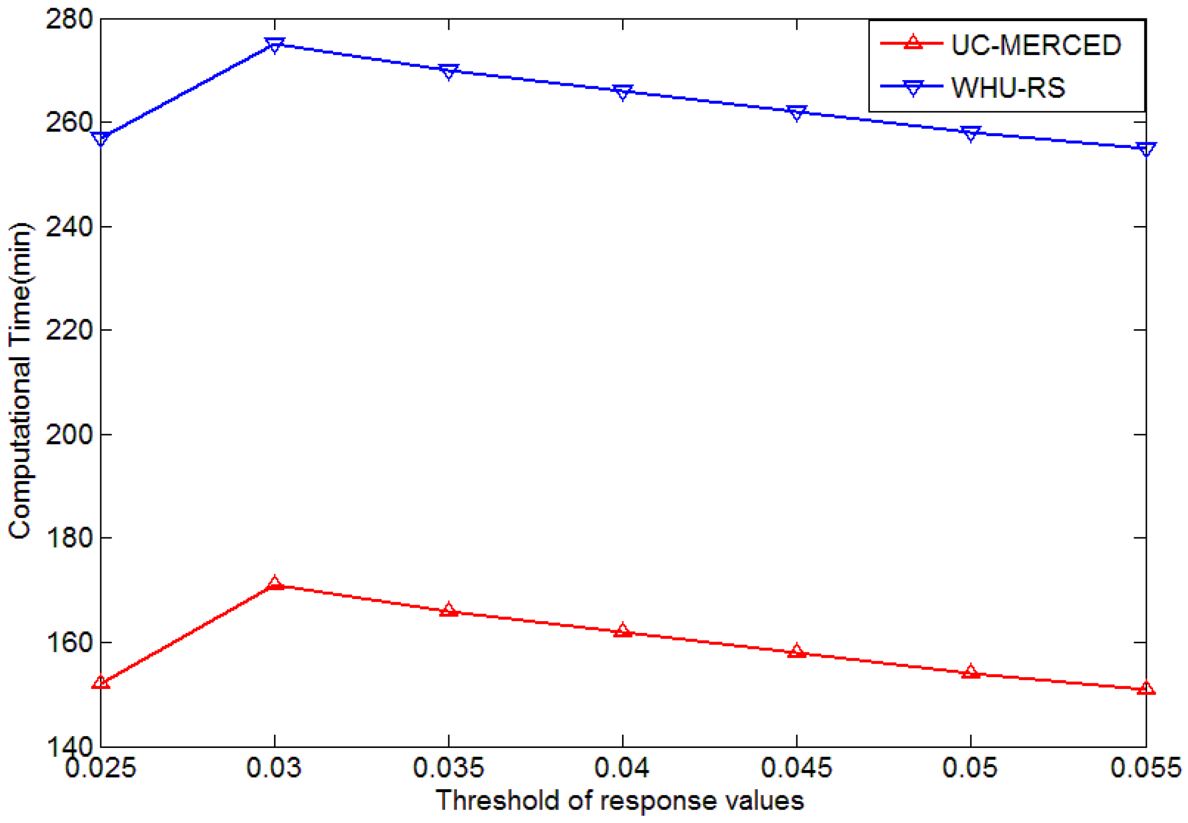
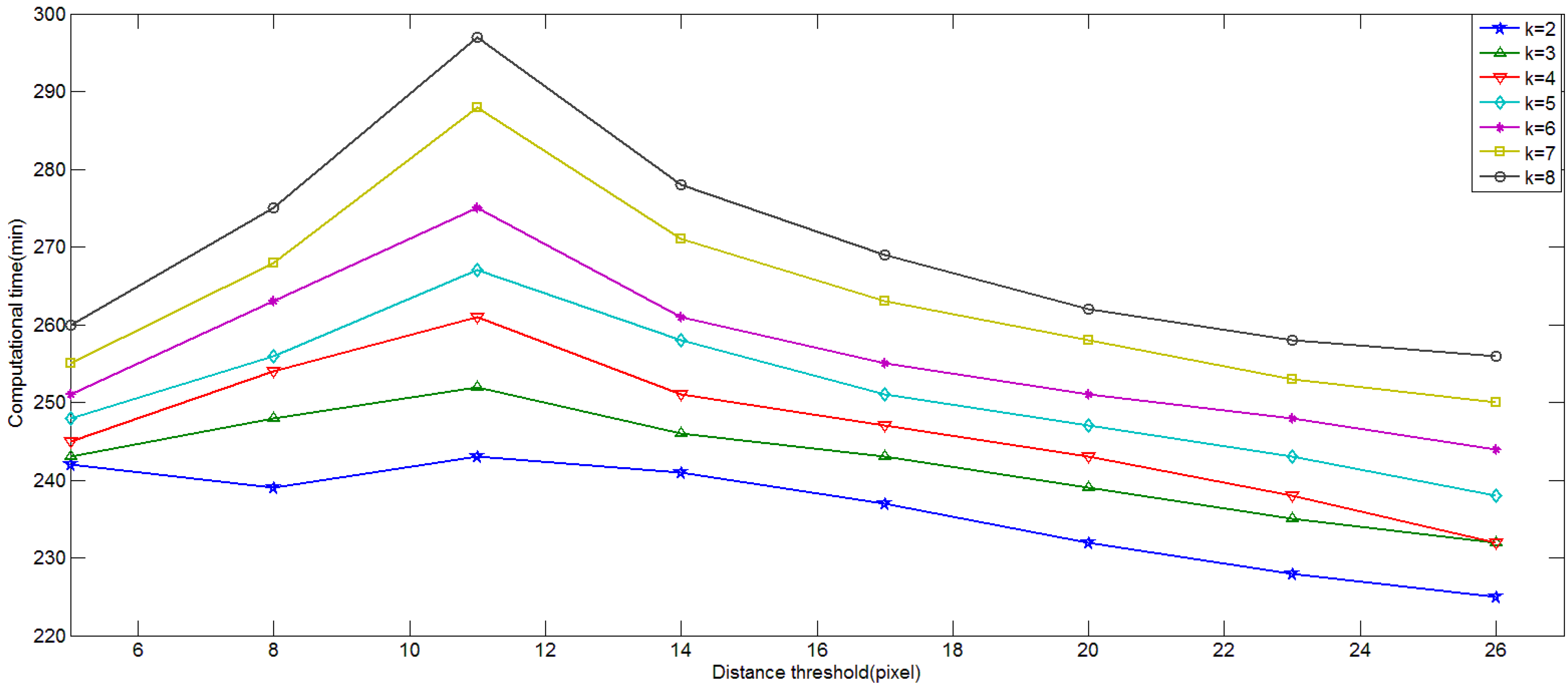
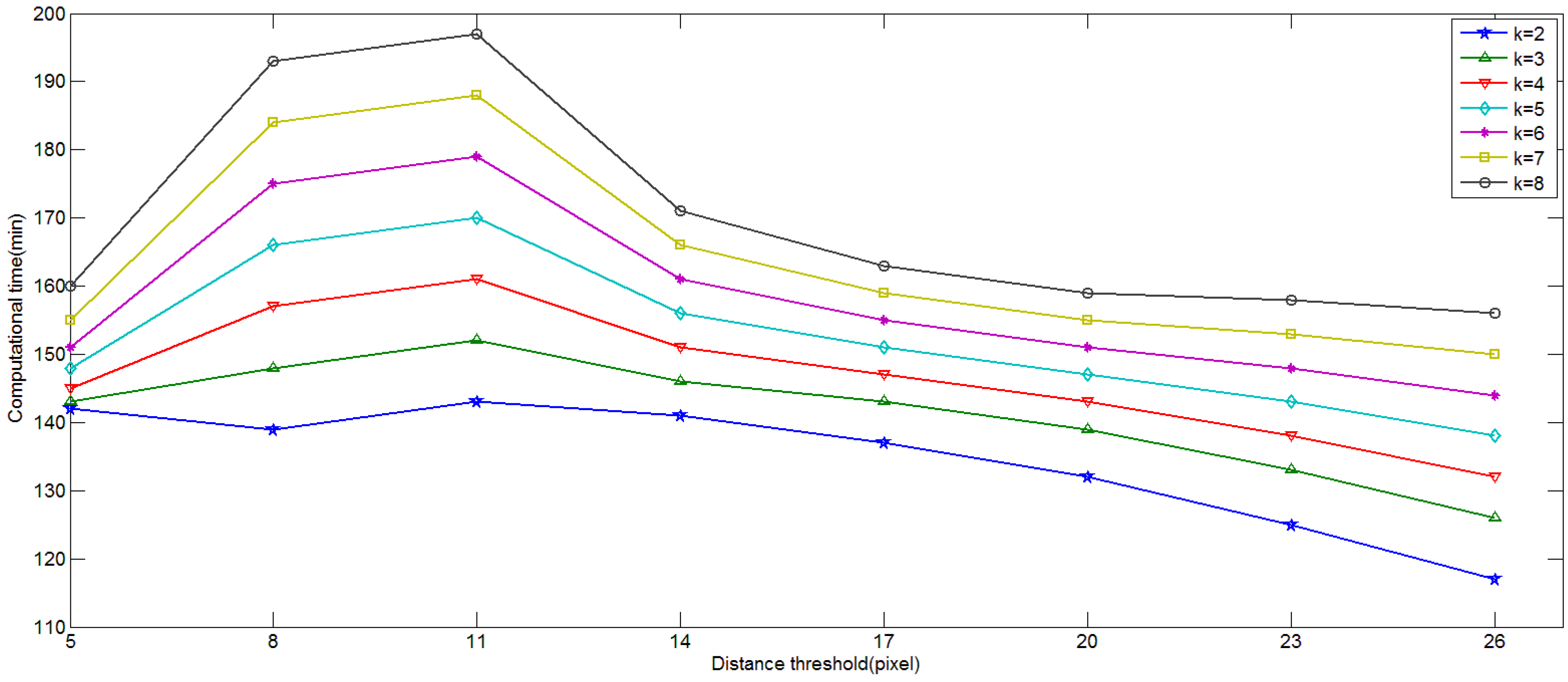
4.1. Influence of Parameters in Keypoint Selection Algorithm

Three parameter settings, threshold of response value, distance threshold and the number of clusters k in “k-means”, will all have an effect on the computational time and classification accuracy. Therefore, contrasting experiments with different parameter settings have been made to find the optimal parameter settings. The main aim of the optimal parameter setting is to achieve higher classification accuracy with less computational time.

Figure 15, Figure 16, Figure 17, Figure 18, Figure 19 and Figure 20 show the computational time and classification accuracy obtained by different parameter settings in the proposed keypoint selection algorithm.

The response value of keypoints ranges from 0.02 to 0.065, so I chose a threshold of response value from 0.025 to 0.055 with an interval of 0.005. Figure 15 and Figure 16 show that, if threshold of response value is equal to 0.025, the computational time reaches the minimum while the best performances in classification accuracy are obtained when threshold is 0.04 in both datasets. However, as we can see in these two pictures, changes in classification accuracy are much more significant and drastic compared with those in computational time. Therefore, we only take classification accuracy into consideration. As can be seen in Figure 16, keypoints with a response value below 0.04 are unstable and not useful for image representation, so removing these key points can help to improve classification accuracy. In the later experiment, 0.04 is selected as the threshold of response value since it performs best in classification with the highest classification accuracy for SVM.

As can be seen in Figure 17 and Figure 18, with distance threshold from 5 to 26 with an interval of 3 since 26 is enough to remove redundant keypoints and number of clusters from 2 to 8, we get the average computational time and classification accuracy. As we can see in Figure 17 and Figure 18, when the number of cluster k is equal to 4 and distance threshold is 14, we can get the highest classification accuracy from SVM while when k is equal to 2 and distance threshold is 26, computational time is the lowest. Similarly, in Figure 15 and Figure 16, the variation yields much more significant changes in classification accuracy than computational time and the threshold corresponding to the lowest computational time performs badly in terms of classification accuracy. Therefore, we choose 4 clusters and a distance threshold of 14, although they take 30 more minutes to achieve the highest classification accuracy for SVM.

Similarly, in Figure 19 and Figure 20, we can reach a similar conclusion to Figure 17 and Figure 18 according to the parameter setting achieving the highest classification accuracy, 4 clusters and distance threshold of 14, although 30 more minutes are spent for better performance in accuracy.

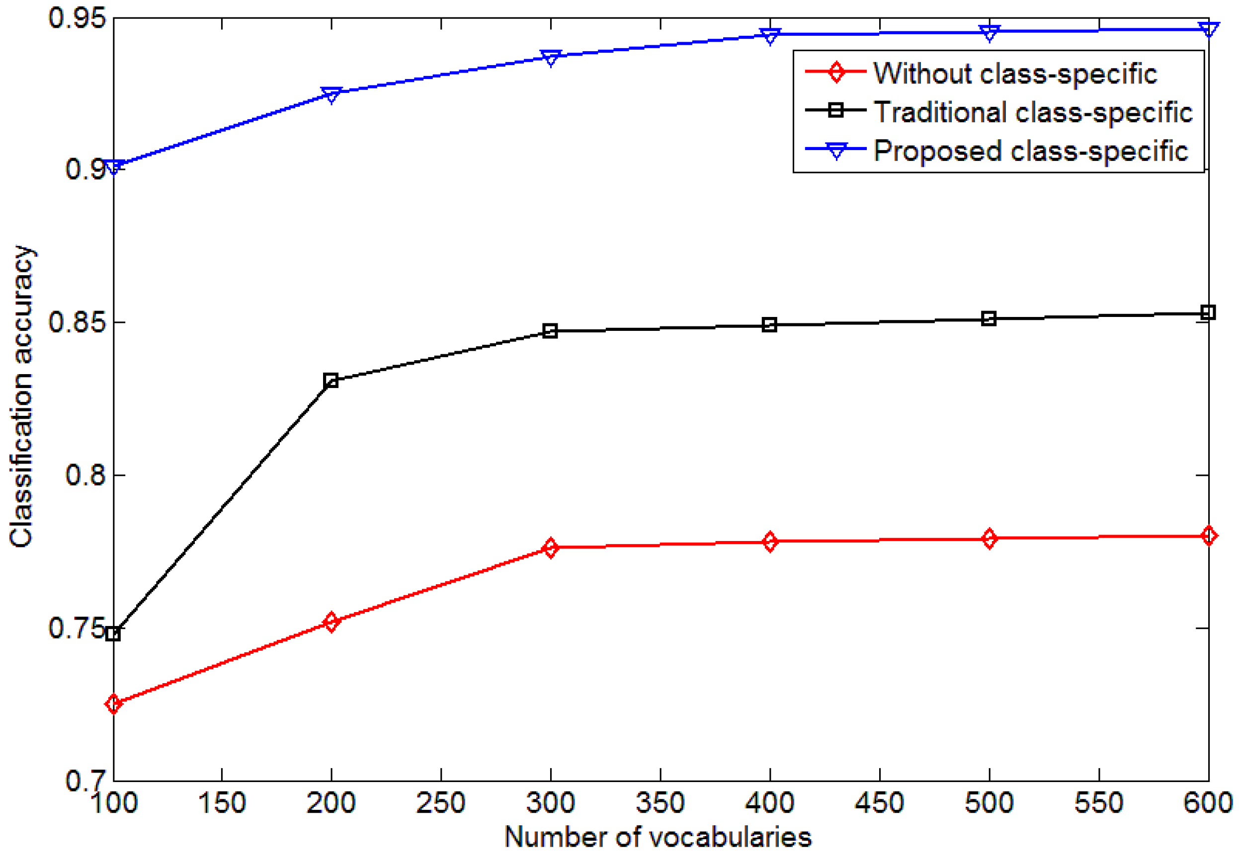
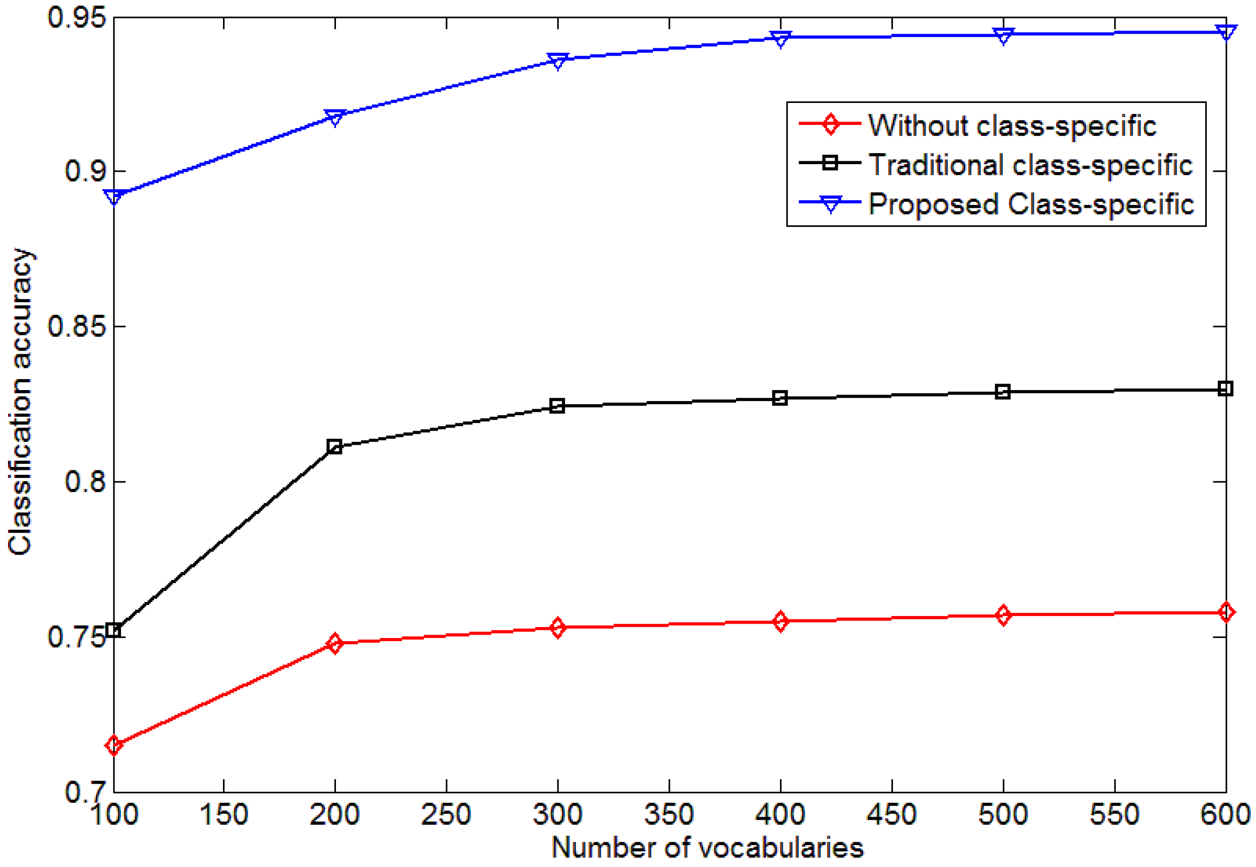
4.2. Influence of the Size of Vocabulary

Different sizes of visual vocabularies were tested on different sizes from 100 to 600 at intervals of 100 since the number of visual words has an effect on classification accuracy.

As can be seen in Figure 21 and Figure 22, the classification accuracy of different methods changes with different sizes of visual vocabularies. When the number of visual vocabularies in all methods increases, classification accuracy improves gradually since a larger class-specific codebook may lead to more detailed image representation. Our proposed algorithm demonstrates a relatively high classification accuracy over all codebook sizes since each category has its unique class-specific codebook, leading to significant difference. The overall accuracy is improved in our proposed algorithm by at least 8% more than for existing methods incorporating the traditional class-specific codebook mentioned in Section 3.1. As we can see, if the visual vocabulary size is over 300, the classification performance improves little, which means a visual vocabulary size of 300 is detailed enough for image representation. Therefore, we choose 400 as the optimal visual vocabulary size for our proposed method.

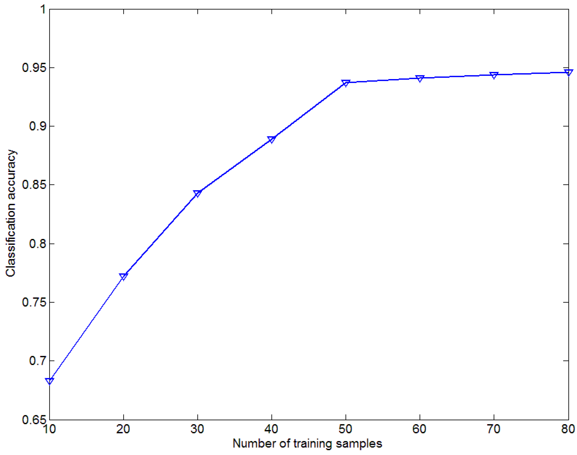
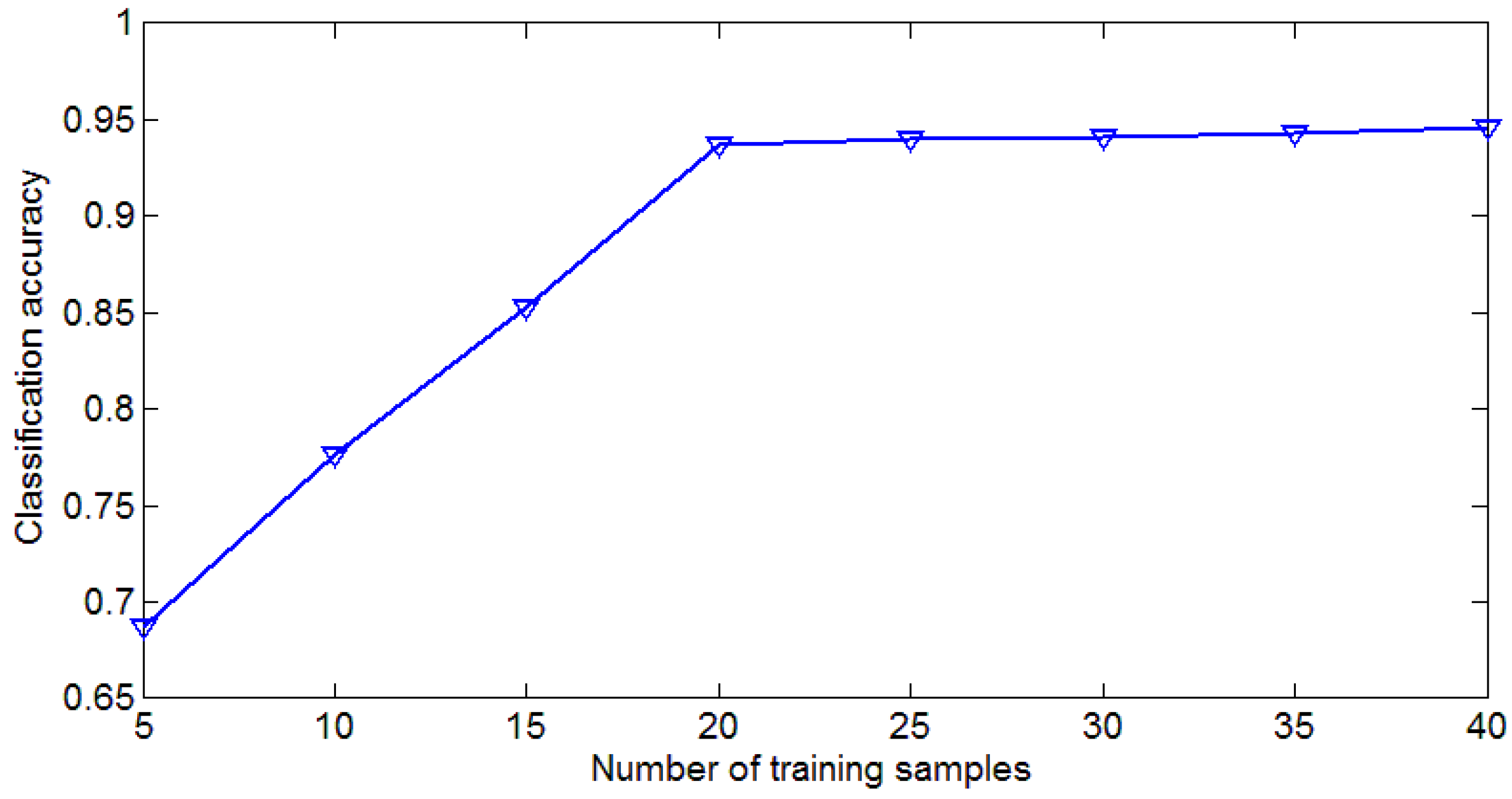
4.3. Influence of Number of Training Samples

A different number of training samples were tested from 10% to 80% of the size of training samples in one category at intervals of 10% since the number of training samples has an effect on classification accuracy.

As can be seen in Figure 23 and Figure 24, classification accuracy improves gradually with the increase of the number of training samples since a larger number of training samples may lead to more accurate caculated MI value. A smaller number of training samples may not fully represent the characteristic of the category, leading to inaccurate assignment of some vocabularies.Therefore, a small number of training samples may result in a relatively inaccurate class-specific codebook in those partly represented categories. As we can see, if the number of training samples is above 50, the classification accuracy improves a little but larger numbers may cost a lot more time. Therefore, we choose 50 training samples for the UC_MERCED dataset. Similarly, in Figure 24, if the number of visual words is below 20, the classification accuracy increases gradually and we choose 20 training samples for WHU-RS dataset.

4.4. Influence of Two-Step Classification

As shown in Figure 9 and Figure 10, testing samples for the KCRC method may misclassify one test sample into its most similar category. Our proposed method results in two labels in KCRC, one is the label with minimum residual and the other is the label with the second minimum residual.

It is more accurate to map universal histogram to class-specific codebooks in these two categories rather than map universal histogram to each category. Two class-specific histograms can be respectively put into the SVM classifier for confidence in each label. Then we do a decision-level fusion to obtain the final classification result. Categories achieving high confidence under both class-specific histograms will be more likely to be the classification result.

For example, the categories of forest and river may have similar backgrounds like trees, which occupy a comparatively large area in one image. Therefore, residuals of forest and river are very close, which may easily result in misclassification. Our proposed method output forest and river as two possible labels. Assuming the testing sample belongs to river, the confidence of river is high in the river class-specific histogram and relatively high in the forest class-specific histogram.

As can be seen in Figure 11, Figure 12, Figure 13 and Figure 14, the two-step classification method demonstrates a little lower accuracy in some categories. There may exist two reasons for this. On one hand, due to insufficient SIFT descriptors extracted from images in these categories, approximately below 100 descriptors, the number of existing visual vocabularies in training images of these two categories is smaller than that in other categories. Therefore, the number of visual words in the class-specific codebook of those two categories is limited and the descriptive ability of these class-specific codebooks is relatively low, thus leading to misclassification. On the other hand, these categories may be similar to at least two other categories. Therefore, both predicted labels are not the true label. Therefore, the output confidence by SVM in both predicted labels is relatively high while the confidence of the true label is relatively low, which may lead to inaccurate classification.

4.5. Strengths and Limitations

A two-step classification method based on a class-specific codebook is proposed in this study. This method has been successfully applied to two datasets of HRIs. The main advantage of the proposed approach is the improvement of computational efficiency in the vector quantization step and increased classification accuracy in the testing samples with similar backgrounds. Experimental results show that this method can achieve an overall classification accuracy of 93.7% and outperforms other state-of-the-art scene-level classification methods.

However, it is noted that some state-of-the-art methods outperform the proposed method in some categories. These categories are short of SIFT features or similar to at least two categories. In future works, we plan to fuse local and global features to decrease the effect of insufficient local descriptors and seek better decision-level fusion methods.

5. Conclusions

Compared with existing BOW methods based on class-specific codebook, our proposed method demonstrates higher classification accuracy than state-of-the-art methods and less computational time compared with methods without keypoint selection. Unlike previous studies that have focused on mapping a universal histogram to each class-specific codebook, we propose a method that classifies the testing image in two steps, predicting two labels of one testing image, and maps the universal histogram to the class-specific codebook in these predicted categories. According to the largest sum of confidence output by the SVM classifier, we can get the final classification results.

The experiments showed the following:

(1)

Modified keypoint selection method is a useful and efficient way to select the discriminative keypoints from extracted descriptors. This method demonstrates lower computational cost and higher classification accuracy.

(2)

We proposed a method for generating class-specific codebook using MI. Vocabularies in the universal codebook will exist in only one specific class-specific codebook. This class-specific codebook will better reflect the information of a specific category.

(3)

By classifying the testing image in two steps, we can decrease the error caused by KCRC. Mapping universal histograms to relatively true labels can help to enlarge the differences between different categories. The proposed two-step classification method outperforms the state-of-the-art methods, in terms of the classification accuracy.

The following research can be taken into consideration in the future. First, descriptors extracted from some images are insufficient for generation of a descriptive class-specific codebook. Therefore, we need to increase the number of visual vocabularies in the class-specific codebook in these categories to enhance descriptive ability. Second, in order to better characterize both local fine details and global structures in images, experiments can be made on fusion of local and global features. Last but not least, we need to seek for better decision-level methods in order to classify testing samples with several similar categories.

References

1. Zhou, V.; Troy, A. An object-oriented approach for analyzing and characterizing urban landscape at the parcel level. Int. J. Remote Sens. 2008, 29, 3119–3135. [Google Scholar] [CrossRef]
2. Zhao, B.; Zhong, Y.; Xia, G.-S.; Zhang, L. Dirichlet-derived multiple topic scene classification model fusing heterogeneous features for high spatial resolution remote sensing imagery. IEEE Trans. Geosci. Remote Sens. 2016, 54, 2108–2123. [Google Scholar] [CrossRef]
3. Zhao, B.; Zhong, Y.; Zhang, L.; Huang, B. The fisher kernel coding framework for high spatial resolution scene classification. Remote Sens. 2016, 8, 157. [Google Scholar] [CrossRef]
4. Akçay, H.G.; Aksoy, S. Automatic detection of geospatial objects using multiple hierarchical segmentations. IEEE Trans. Geosci. Remote Sens. 2008, 46, 2097–2111. [Google Scholar] [CrossRef] [Green Version]
5. Xia, G.S.; Hu, J.; Hu, F.; Shi, B.; Bai, X.; Zhong, Y.; Zhang, L. AID: A benchmark dataset for performance evaluation of aerial scene classification. ArXiv preprint 2016. [Google Scholar]
6. Lowe, D.G. Distinctive image features from scale-invariant keypoints. Int. J. Comput. Vis. 2004, 60, 91–110. [Google Scholar] [CrossRef]
7. Ojala, T.; Pietikainen, M.; Maenpaa, T. Multi-resolution gray-scale and rotation invariant texture classification with local binary patterns. IEEE Trans. Pattern Anal. Mach. Intell. 2002, 24, 971–987. [Google Scholar] [CrossRef]
8. Swain, M.J.; Ballard, D.H. Color indexing. Int. J. Comput. Vis. 1991, 7, 11–32. [Google Scholar] [CrossRef]
9. Oliva, A.; Torralba, A. Building the gist of a scene: The role of global image features in recognition. Prog. Brain Res. 2006, 155, 23–36. [Google Scholar] [PubMed]
10. Csurka, G.; Dance, C.; Fan, L.; Willamowski, J.; Bray, C. Visual categorization with bags of keypoints. In Proceedings of the Workshop on Statistical Learning in Computer Vision, Washington, DC, USA, 28 June 2004.
11. Blei, D.M.; Ng, A.Y.; Jordan, M.I. Latent dirichlet allocation. J. Mach. Learn. Res. 2003, 3, 993–1022. [Google Scholar]
12. Bosch, A.; Zisserman, A.; Muñoz, X. Scene classification via pLSA. In Proceedings of the European Conference on Computer Vision, Graz, Austria, 7–13 May 2006; pp. 517–530.
13. Russakovsky, O.; Deng, J.; Su, H.; Krause, J.; Satheesh, S.; Ma, S.; Huang, Z.; Karpathy, A.; Khosla, A.; Bernstein, M.S.; et al. ImageNet large scale visual recognition challenge. Int. J. Comput. Vis. 2015, 115, 211–252. [Google Scholar] [CrossRef]
14. Luus, F.P.S.; Salmon, B.P.; Van Den Bergh, F.; Maharaj, B.T.J. Multiview deep learning for land-use classification. IEEE Geosci. Remote Sens. Lett. 2015, 12, 2448–2452. [Google Scholar] [CrossRef]
15. Sermanet, P.; Eigen, D.; Zhang, X.; Mathieu, M.; Fergus, R.; Lecun, Y. Overfeat: Integrated recognition, localization and detection using convolutional networks. ArXiv preprint 2013. [Google Scholar]
16. Jia, Y.; Shelhamer, E.; Donahue, J.; Karayev, S.; Long, J.; Girshick, R.; Guadarrama, S.; Darrell, T. Caffe: Convolutional architecture for fast feature embedding. In Proceedings of the 22nd ACM international conference on Multimedia, Orlando, FL, USA, 3–7 November 2014; pp. 675–678.
17. Szegedy, C.; Liu, W.; Jia, Y.; Sermanet, Y.; Reed, S.; Anguelov, D.; Dumitru, E.; Vanhoucke, V.; Rabinovich, A. Going deeper with convolutions. In Proceedings of the IEEE Conference on Computer Vision and Pattern Recognition, Boston, MA, USA, 7–12 June 2015; pp. 1–9.
18. Yang, Y.; Newsam, S. Bag-of-visual-words and spatial extensions for land-use classification. In Proceedings of the 18th SIGSPATIAL International Conference on Advances in Geographic Information Systems, San Jose, CA, USA, 3–5 November 2010; pp. 270–279.
19. Cheng, G.; Guo, L.; Zhao, T.; Han, J.; Li, H.; Fang, J. Automatic landslide detection from remote-sensing imagery using a scene classification method based on BoVW and pLSA. Int. J. Remote Sens. 2013, 34, 45–59. [Google Scholar] [CrossRef]
20. Turcot, P.; Lowe, D. Better matching with fewer features: The selection of useful features in large database recognition problems. In Proceedings of the ICCV Workshop on Emergent Issues in Large Amounts of Visual Data (WS-LAVD), Kyoto, Japan, 4 October 2009.
21. Perronnin, F. Universal and adapted vocabularies for generic visual categorization. IEEE Trans. Pattern Anal. Mach. Intell. 2008, 30, 1243–1256. [Google Scholar] [CrossRef] [PubMed]
22. Dorko, G.; Schmid, C. Selection of scale-invariant parts for object class recognition. In Proceedings of the IEEE International Conference on Computer Vision, Nice, France, 13–16 October 2003; pp. 634–639.
23. Vidal-Naquet, M.; Ullman, S. Object recognition with informative features and linear classification. In Proceedings of the IEEE International Conference on Computer Vision, Nice, France, 13–16 October 2003; pp. 281–288.
24. Agarwal, S.; Roth, D. Learning a sparse representation for object detection. In Proceedings of the European Conference on Computer Vision, Copenhagen, Denmark, 28–31 May 2002; pp. 113–130.
25. Chin, T.-J.; Suter, D.; Wang, H. Boosting histograms of descriptor distances for scalable multiclass specific scene recognition. Image Vis. Comput. 2011, 29, 2. [Google Scholar] [CrossRef]
26. Opelt, A.; Pinz, M.; Fussenegger, P. Auer, Generic object recognition with boosting. IEEE Trans. Pattern Anal. Mach. Intell. 2006, 28, 416–431. [Google Scholar] [CrossRef] [PubMed]
27. Lin, W.C.; Tsai, C.F.L.; Chen, Z.Y.; Ke, S. Keypoint selection for efficient bag-of-words feature generation and effective image classification. Inf. Sci. 2016, 329, 33–51. [Google Scholar] [CrossRef]
28. Altintakan, U.L.; Yazici, A. Towards effective image classification using class-specific codebooks and distinctive local features. IEEE Trans. Multimed. 2015, 17, 323–332. [Google Scholar] [CrossRef]
29. Li, H.; Yang, L.; Guo, C. Improved piecewise vector quantized approximation based on normalized time subsequences. Measurement 2013, 46, 3429–3439. [Google Scholar] [CrossRef]
30. Wright, J.; Yang, A.; Sastry, S.; Ma, Y. Robust face recognition via sparse representation. IEEE Trans. Pattern Anal. Mach. Intell. 2009, 31, 210–227. [Google Scholar] [CrossRef] [PubMed]
31. Suykens, J.A.K.; Vandewalle, J. Least squares support vector machine classifiers. Neural Process. Lett. 1999, 9, 293–300. [Google Scholar] [CrossRef]
32. Lazebnik, S.; Schmid, C.; Ponce, J. Beyond bags of features: Spatial pyramid matching for recognizing natural scene categories. In Proceedings of the 2006 IEEE Computer Society Conference on Computer Vision and Pattern Recognition, Washington, DC, USA, 17–22 June 2006; Volume 2, pp. 2169–2178.
33. Wang, J.; Yang, J.; Yu, K.; Lv, F.; Huang, T.; Gong, T. Locality-constrained linear coding for image classification. In Proceedings of the IEEE Computer Society Conference on Computer Vision and Pattern Recognition, San Francisco, CA, USA, 13–18 June 2010; pp. 3360–3367.
34. Yang, J.; Yu, K.; Gong, Y.; Huang, T. Linear spatial pyramid matching using sparse coding for image classification. In Proceedings of the IEEE Computer Society Conference on Computer Vision and Pattern Recognition, Miami, FL, USA, 20–25 June 2009.
35. Yuan, Q.; Zhang, L.; Shen, H. Hyperspectral image denoising employing a spectral-spatial adaptive total variation model. IEEE Trans. Geosci. Remote Sens. 2012, 50, 3660–3677. [Google Scholar] [CrossRef]
36. Zhang, L.; Yang, M.; Feng, X. Sparse representation or collaborative representation: Which helps face recognition? In Proceedings of the IEEE 2011 International Conference on Computer Vision, Colorado Springs, CO, USA, 20–25 June 2011; pp. 471–478.
37. Sheng, G.; Yang, W.; Xu, T.; Sun, H. High-resolution satellite scene classification using a sparse coding based multiple feature combination. Int. J. Remote Sens. 2011, 33, 2395–2412. [Google Scholar] [CrossRef]
38. Chang, C.C.; Lin, C.J. LIBSVM: A Library for Support Vector Machines. 2001. Available online: http://www.csie.ntu.edu.tw/~cjlin/libsvm (accessed on 30 May 2013).
39. Hsu, C.W.; Lin, C.J. A comparison of methods for multiclass support vector machines. IEEE Trans. Neural Netw. 2002, 13, 415–425. [Google Scholar] [PubMed]
40. Aha, D.W.; Kibler, D.; Albert, M.K. Instance-based learning algorithms. Mach. Learn. 1991, 6, 37–66. [Google Scholar] [CrossRef]
41. Wilson, D.R.; Martinez, T.R. Reduction techniques for instance-based learning algorithms. Mach. Learn. 2000, 38, 257–286. [Google Scholar] [CrossRef]
42. Brighton, H.; Mellish, C. Advances in instance selection for instance-based learning algorithms. Data Min. Knowl. Discov. 2002, 6, 153–172. [Google Scholar] [CrossRef]
43. Perronnin, F.; Sánchez, J.; Mensink, T. Improving the fisher kernel for large-scale image classification. In Proceedings of the European Conference on Computer Vision, Crete, Greece, 5–11 September 2010; pp. 143–156.
44. Negrel, R.; Picard, D.; Gosselin, P.H. Evaluation of second-order visual features for land-use classification. In Proceedings of the 2014 12th International Workshop on Content-Based Multimedia Indexing (CBMI), Klagenfurt, Austria, 18–20 June 2014; pp. 1–5.
Figure 1. (a) Original Scale-Invariant Feature Transform (SIFT) features extracted from images (b) keypoint selection results using modified keypoint selection method presented in this text.
Remotesensing 09 00223 g001
Figure 2. Similar categories that traditional bag-of-words (BOW) may misclassify (a) Forest and river (b) Forest and chaparral (c) Freeway and airport.
Remotesensing 09 00223 g002
Figure 3. Differences between error terms of existing methods incorporating scene labels and our proposed method.
Remotesensing 09 00223 g003
Figure 4. Overview of the improved class-specific BOW model for land-use scene classification.
Remotesensing 09 00223 g004
Figure 5. Central idea of removing keypoints (a) Clustered keypoints with “k-means” in SIFT feature space. (b) Original keypoints in one cluster (c) Selected keypoints with a distance threshold.
Remotesensing 09 00223 g005
Figure 6. Procedure of generating class-specific histogram.
Remotesensing 09 00223 g006
Figure 7. Examples of ground truth data in the UC_MERCED dataset.
Remotesensing 09 00223 g007
Figure 8. Examples of ground truth data in the WHU-RS dataset.
Remotesensing 09 00223 g008
Figure 9. Two Example images of categories misclassified with KCRC method but classified accurately with two-step classification method in WHU-RS dataset.
Remotesensing 09 00223 g009
Figure 10. Two Example images of categories misclassified with KCRC method but classified accurately with two-step classification method in UC_MERCED dataset.
Remotesensing 09 00223 g010
Figure 11. Classification accuracy per class for classifiers using UC_MERCE dataset. The class labels are assigned as follows: 1 = Agricultural, 2 =airplane, 3 = baseball diamond, 4 = beach, 5 = buildings, 6 = chaparral, 7 =dense residential, 8 = forest, 9 = freeway, 10 = golf course, 11 = harbor, 12 = intersection, 13 = medium residential, 14 = mobile home park, 15 =overpass, 16 = parking lot, 17 = river, 18 = runway, 19 = sparseresidential,20 = storage tanks, and 21 = tennis court.
Remotesensing 09 00223 g011
Figure 12. Classification accuracy per class for classifiers using WHU-RS dataset. The rows and columns of the matrix denote the actual and predicted classes, respectively. The class labels are assigned as follows: 1 = airport, 2 = beach, 3 = bridge, 4 = commercial, 5 = desert, 6 = farmland, 7 = football field, 8 = forest, 9 = industrial, 10 = meadow, 11 = mountain, 12 = park, 13 = parking, 14 = pond, 15 = port, 16= railway station, 17 = residential, 18 = river, 19 = viaduct.
Remotesensing 09 00223 g012
Figure 13. Confusion matrix for the proposed algorithm using WHU-RS land-use dataset.
Remotesensing 09 00223 g013
Figure 14. Confusion matrix for the proposed algorithm using UC_MERCED land-use dataset.
Remotesensing 09 00223 g014
Figure 15. Computational time for vector quantization with different thresholds of response value.
Remotesensing 09 00223 g015
Figure 16. Classification accuracy with different thresholds of response value.
Remotesensing 09 00223 g016
Figure 17. Classification accuracy with different distance thresholds and number of clusters over WHU-RS dataset.
Remotesensing 09 00223 g017
Figure 18. Computational time for generating BOW features with different distance thresholds and number of clusters over WHU-RS dataset.
Remotesensing 09 00223 g018
Figure 19. Computational time for generating BOW features with different distance thresholds and the number of clusters over UC_MERCED dataset.
Remotesensing 09 00223 g019
Figure 20. Classification accuracy with different distance thresholds and number of clusters over UC_MERCED dataset.
Remotesensing 09 00223 g020
Figure 21. Classification accuracy with a different number of visual words in WHU-RS datasets.
Remotesensing 09 00223 g021
Figure 22. Classification accuracy with a different number of visual words in UC_MERCED land-use dataset.
Remotesensing 09 00223 g022
Figure 23. Overall accuracies using different number of training samples in UC_MERCED dataset.
Remotesensing 09 00223 g023
Figure 24. Overall accuracies using different number of training samples in WHU-RS dataset.
Remotesensing 09 00223 g024