Transferring Pre-Trained Deep CNNs for Remote Scene Classification with General Features Learned from Linear PCA Network

Abstract

Deep convolutional neural networks (CNNs) have been widely used to obtain high-level representation in various computer vision tasks. However, in the field of remote sensing, there are not sufficient images to train a useful deep CNN. Instead, we tend to transfer successful pre-trained deep CNNs to remote sensing tasks. In the transferring process, generalization power of features in pre-trained deep CNNs plays the key role. In this paper, we propose two promising architectures to extract general features from pre-trained deep CNNs for remote scene classification. These two architectures suggest two directions for improvement. First, before the pre-trained deep CNNs, we design a linear PCA network (LPCANet) to synthesize spatial information of remote sensing images in each spectral channel. This design shortens the spatial “distance” of target and source datasets for pre-trained deep CNNs. Second, we introduce quaternion algebra to LPCANet, which further shortens the spectral “distance” between remote sensing images and images used to pre-train deep CNNs. With five well-known pre-trained deep CNNs, experimental results on three independent remote sensing datasets demonstrate that our proposed framework obtains state-of-the-art results without fine-tuning and feature fusing. This paper also provides baseline for transferring fresh pre-trained deep CNNs to other remote sensing tasks.

1. Introduction

Remote sensing image processing achieves great advances in recent years, from low-level tasks, such as segmentation, to high-level ones, such as classification [1,2,3,4,5,6,7]. However, the task becomes incrementally more difficult as the level of abstraction increases, going from pixels, to objects, and then scenes. Classifying remote sensing images according to a set of semantic categories is a very challenging problem, because of high intra-class variability and low inter-class distance [5,6,7,8,9]. Different objects may appear at different scales and orientations in a given class, and the same objects may be found in images belonging to different classes. By constructing a holistic scene representation, the bag-of-visual-words (BOW) model becomes one of the most popular approaches for solving the scene classification problem in the remote sensing community [10]. In addition, many variant methods based on the BOW model have been developed for improving the discriminative ability of the “visual words” [11,12,13]. Nevertheless, the representations generated from BOW are still in mid-level form and not sufficiently powerful for scene classification. Therefore, more representative and higher-level representations are desirable and will certainly play a dominant role in scene-level tasks.

Deep learning algorithm attempts to learn high-level features corresponding to high level of abstraction. The deep convolutional neural network (CNN) [14], which is acknowledged as the most successful and widely used deep learning model, is now the dominant method in the majority of recognition and detection tasks. Its recent impressive results for computer vision applications bring dramatic improvements beyond the state-of-the-art records on a number of benchmarks [15,16,17,18]. In remote sensing field, the use of deep learning is rapidly growing. A considerable number of works propose deep strategies for spatial and spectral feature learning [3,19,20,21]. Vakalopoulou et al. [3] propose an automated building detection framework from very high resolution remote sensing data based on deep convolutional neural networks. In [19], deep convolutional neural networks are employed to classify hyperspectral images directly in spectral domain. In addition, Makantasis et al. [20] propose a deep learning based method that exploits a CNN to encode pixels’ spectral and spatial information and constructs high-level features of hyperspectral data in an automated way. Furthermore, Hamida et al. [21] design a lightweight CNN architecture to process spectral and spatial information of hyperspectral data, and provide a less costing solution while ensuring an accurate classification of the hyperspectral data. In theory, considering the subtle differences among categories in remote scene classification, we may attempt to form high-level representations for remote sensing images from CNN activations. However, the acquisition of large-scale well-annotated remote sensing image datasets is costly, and it is easy to over-fit when we try to train a high-powered deep CNN with small datasets in practice [22]. On the other hand, even though we have obtained large enough remote sensing datasets, learning billions parameters in these deep CNNs is very time-consuming.

ImageNet (http://www.image-net.org/challenges/LSVRC/) is a large-scale dataset, which offers a very comprehensive database of more than 1.2 million categorized natural images of 1000+ classes [23]. Deep CNN models trained upon this dataset serve as the backbone for many segmentation, detection and classification tasks on other datasets. Moreover, some very recent works have demonstrated that the representations learned from deep CNNs pre-trained on large datasets such as ImageNet can be transferable to image classification task [24]. Some works also start to apply them to remote sensing field, and obtain state-of-the-art results for some specific datasets [22,25,26]. Penatti et al. [25] evaluate the generalization power of experimentally CNNs trained for recognizing everyday objects for the classification of remote sensing images. Castelluccio et al. [22] explore the use of pre-trained deep CNNs for the classification of remote scenes. The pre-trained networks are fine-tuned on the target data, to avoid overfitting problems and reduce design time. In [26], features from various successfully pre-trained deep CNNs are transferred for remote scene classification. Via extracting CNN features from different layers, the proposed framework results in remarkable performance even with a simple linear classifier. However, the generalization power of deep features learned from deep CNNs fades evidently when the features of remote sensing images become different in space and spectrum with that of natural images in the ImageNet dataset [22,25]. Therefore, a foreseeable question is that how can we further enhance the generalization power of pre-trained deep CNNs for remote sensing imagery.

PCA network (PCANet) is a simple but effective neural network, which mainly comprises three components: cascaded principal component analysis (PCA), binary hashing, and block-wise histograms [27]. In the PCANet model, there are no nonlinear operations in its early stages, until the very last output layer. Moreover, filters learning in the PCANet does not involve regularized parameters or require numerical optimization solvers. Namely, it is unsupervised. In our experiments, we apply a simple and shallow linear PCANet to the remote sensing images before transferring the pre-trained deep CNNs to them. We find that features learned from this framework improve the remote scene classification performance. To our surprise, this framework works well even in the condition that the remote sensing images are very different in space and spectrum with the natural images from ImageNet dataset that is used to pre-train the deep CNNs. Inspired by this, we evaluate the performance of this framework for remote scene classification in different conditions, and explore the way in which the LPCANet synthesizes spatial and spectral information of remote sensing images and enhances the generalization power of pre-trained deep CNNs.

Therefore, in our work, we propose a framework to obtain general features from the pre-trained deep CNNs for remote scene classification and attempt to form a baseline for transferring pre-trained deep CNNs to remote sensing images with various spatial and spectral information. By applying a shallow LPCANet to the remote sensing images, we generate features with particular spatial and spectral form, which serve as inputs of the pre-trained deep CNN. Then, we remove the output layer of the pre-trained deep CNN and see the remainder of it as a fixed feature extractor. The obtained features of the image scenes are fed into a simple classifier for the scene classification task. We propose two scenarios to test the performance of the LPCANet on extracting general features for pre-trained deep CNNs in space and spectrum, respectively:

(1)

By applying a shallow LPCANet to each spectral channel of the remote sensing images, we test the performance of LPCANet on extracting general features for pre-trained CNNs in spatial information.

(2)

Furthermore, we introduce quaternion algebra to LPCANet and design the linear quaternion PCANet (LQPCANet) to further extract general features for pre-trained CNNs from spectral information and test its performance for different remote sensing images.

We conduct extensive experiments with different pre-trained deep CNNs such as CaffeNet [17], GoogLeNet [28] and ResNet [29]. Based on various pre-trained deep CNNs, we evaluate our proposed framework on different remote sensing datasets that vary in space and spectrum. The results show that our proposed framework can enhance the generalization power of pre-trained deep CNNs and learn better features for remote scenes. With “unsupervised settings”, our proposed framework achieves state-of-the-art performance on some public remote scene datasets.

Our proposed framework hardly contains any deep or new techniques, and our study so far is mainly empirical. However, a thorough report on such a baseline system has tremendous value for transferring pre-trained deep CNNs to remote sensing images that vary in space and spectrum. Our main contributions are summarized as follows:

(1)

We thoroughly investigate how the LPCANet and LQPCANet synthesize spatial and spectral information of the remote sensing imagery and how can them enhance generalization power of pre-trained deep CNNs for remote scene classification.

(2)

For future study, our proposed framework can serve as a simple but surprisingly effective baseline for empirically justifying advanced designs of transferring pre-trained deep CNNs to remote sensing images. We can take any pre-trained deep CNN as a starting point and improve the network further with our proposed method.

(3)

Our proposed features learning framework is under the “unsupervised settings”, which is an encouraging orientation in deep learning, and is more promising for remote sensing tasks compared with supervised or semi-supervised method.

The rest of the paper is organized as follows. Section 2 provides the whole framework of our proposed method. Section 2.1 presents successful pre-trained deep CNNs nowadays and the development of them. Section 2.2 introduces LPCANet and its quaternion representation, which form the foundation of our proposed two architectures explained in Section 2.3. Experiments are presented in Section 3 and we conclude the paper in Section 4 with some remarks in Section 5.

2. Enhancing the Generalization Power of Pre-Trained Deep CNNs for Remote Scene Classification

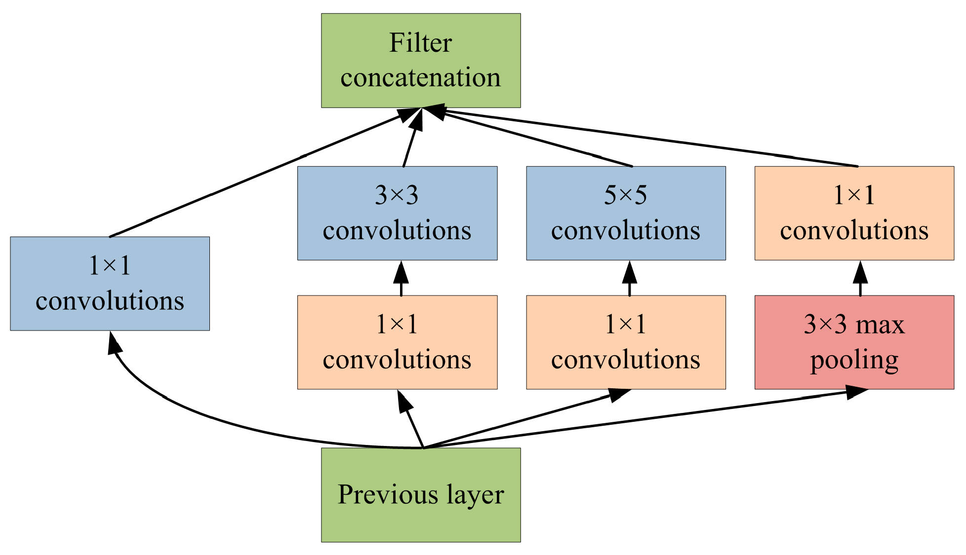
2.1. Pre-Trained Deep Convolutional Neural Networks

According to the biological template discovered by Hubel and Wiesel in 1959, the visual cortex of our brain is organized in layers [30]. The lower layers extract basic features of images, such as spots, lines, and corners. The higher layers combine these basic features to form templates that are more complex. Inspired by this, Fukushima [31] first proposed the convolutional neural networks in 1980, which was then refined by LeCun in 1989 [32]. Thanks to fast growth of affordable computing power, especially graphical processing units (GPUs), and the diffusion of large datasets of labeled images for training, a seminal deep convolutional neural network called AlexNet won the 2012 ImageNet Large Scale Visual Recognition Challenge (ILSVRC-2012) [33], and brought increasing interest for deep CNNs in the last few years. The typical architecture of a deep CNN is composed of multiple cascaded layers with various types. The convolutional layers convolve input feature maps with a set of weights (also called kernels or filters) to generate new feature maps. The deeper convolutional layers are able to learn features that are more abstract by combining lower-level ones learned in former layers. After convolutional layer, a non-linear activation function, such as sigmoid unit, is applied to improve generalization of learned feature maps. The pooling layers perform downsampling operation on local regions of feature maps to reduce the dimension of input feature maps and provide translation invariance at the same time. The fully-connected layers finally follow several stacked convolutional and pooling layers, and the last fully-connected layer is a Softmax layer that computes the scores for each defined class. The parameters of CNNs are typically trained with classic stochastic gradient descent based on the backpropagation algorithm. With well trained parameters, CNNs transform the input images to high-level feature maps in a feedforward manner.

Based on the typical deep CNN, AlexNet replaces the sigmoid unit with the rectified linear unit (ReLU), which allows much faster training. On the other hand, it uses dropout technique to alleviate the effect of over-fitting [15]. Moreover, CaffeNet further places the non-linear activation functions after pooling layers [17]. Very recently, there are two major directions, in which a lot of efforts are made to update the typical deep CNN, and drive it to achieve better performance in computer vision tasks.

The first direction is to make CNNs deeper. VGG-VD networks developed by Simonyan et al. [18] are very deep CNN models, which won the runner-up in ILSVRC-2014. Known as two successful very deep CNN models, VGG-VD16 and VGG-VD19 demonstrate that the depth of the network plays a significant role in improving classification accuracy. Furthermore, MSRA-Net is designed deeper by replacing the 5 × 5 filters with two series 3 × 3 filters [34]. It achieves better performance and reduces computational complex at the same time.

The other direction is to renovate the typical layers in deep CNNs. Network in Network (NIN) [35] replaces the linear convolutional layer with multilayer perceptron called MLPconv layer. In addition, instead of fully-connected layers, it uses global average pooling to obtain output features. GoogLeNet is the CNN architecture that won the ILSVRC-2014 competition, which contains 24 layers [28]. Inspired by “Network in Network” idea, it uses the inception modules as shown in Figure 1, which employs filters of different sizes at each layer and reduces the number of parameters at the same time. Furthermore, the inception module is modulated in the CNN architecture of Inception V3 [36], in which two series 3 × 3 filters are used to take place of the 5 × 5 filters. Moreover, 1 × n and n × 1 convolutional kernels derived from n × n operation reduce parameters in the network and economize the computational cost. Figure 2 depicts the changes of inception module in the architecture of Inception V3. Derived from the architecture of Inception V3, Inception V4 network benefits from new inception module, which is more complex and deeper [37].

By integrating the two directions discussed above, deep residual network (ResNet) [29] that won the 1st place in the ILSVRC-2015 reformulates the layers in it as learning residual functions with reference to layer inputs, instead of learning unreferenced functions such as convolutional operation. At the same time, it is easy to optimize, and can gain accuracy from increased depth. ResNet achieves great success on the ImageNet dataset with a depth of up to 152 layers—8× deeper than VGG nets. Based on ResNet, identity mapping residual net further optimizes the residual learning framework, and achieves better performance with considerable margin [37].

In summary, Figure 3 briefly demonstrates the evolution of CNNs’ structure. Not strictly separated, the two channels in Figure 3 are used to depict the two mainstream ideas in which typical deep CNN is updated to achieve successful performance.

However, these successful deep CNNs discussed above do not achieve good performance as we expected, when we directly apply them to remote sensing images. In fact, almost all successful deep CNNs are trained on daily natural image datasets, such as ImageNet [23], because huge amounts of labeled daily images are available online. In the field of remote sensing, limited training data in remote sensing datasets brings overfitting when we attempt to train a deep CNN, and the deep CNN trained by limited training data dose not generalize well to test data.

An effective solution, recently explored in [22,25,26], is to transfer deep features trained on ImageNet dataset to remote sensing images. This solution derives from that, in the lower layers of a deep CNN, features learned from both the daily nature images and remote sensing images are alike, such as blobs and edges. These features are general enough to be useful in both the two kinds of datasets, and thus the high-level features in deep CNNs computed from daily nature images may be powerful representations for remote sensing images. However, this transferring operation depends on an important principle: the “distance” of the source dataset on which the deep CNN is trained and the target dataset to which the deep features are transferred should be small enough. In this paper, we define “distance” as the degree of difference in spatial and spectral information between source and target datasets. In order to reduce the “distance” between remote sensing images and daily nature images, we design LPCANet and LQPCANet to synthesize the spatial and spectral information of remote sensing images respectively. By doing this, the generalization power of CNN pre-trained on ImageNet is enhanced for remote scene classification.

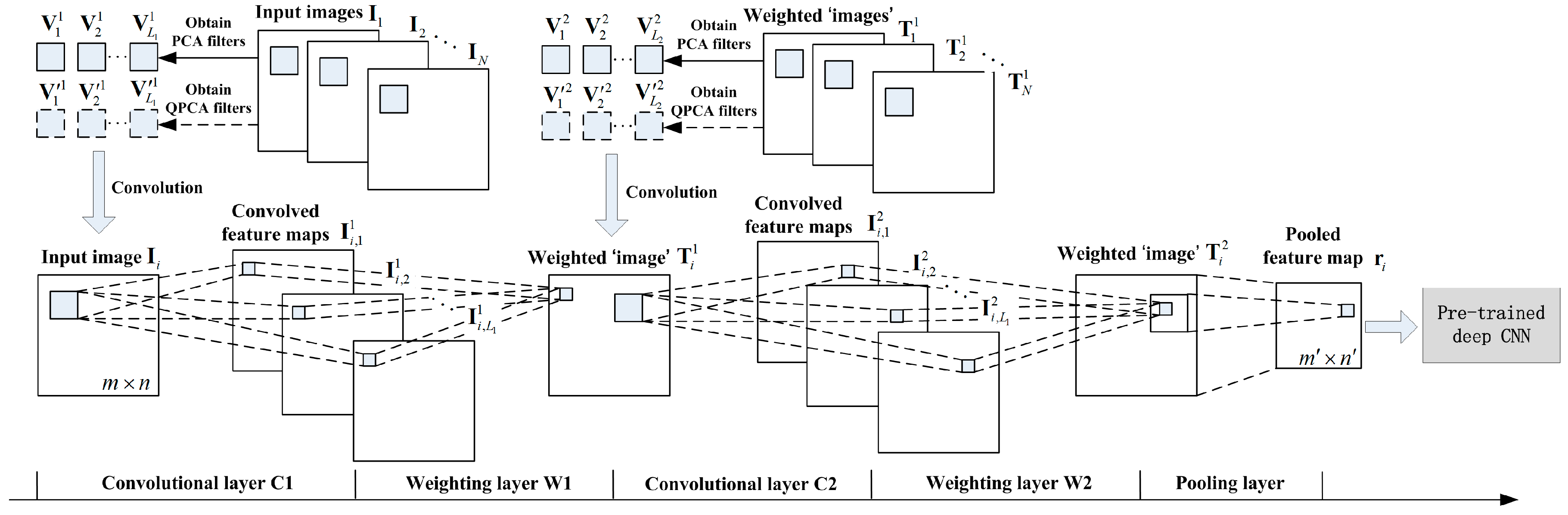
2.2. LPCANet and Its Quaternion Representation

In this section, we design the structure of LPCANet, which derives from the PCANet [27]. We try to synthesize spatial information of remote sensing images through it. On the other hand, we introduce the quaternion algebra into LPCANet, and further synthesize spectral information of remote sensing images. Stage of hashing and histograms in PCANet is replaced by stages of weighting and hashing in LPCANet and LQPCANet to guarantee the linear property throughout all the operations in them. By doing this, the principle features of remote sensing images are learned and then sent to deep CNNs, which are pre-trained on large-scale datasets such as ImageNet [23]. The structure of LPCANet (LQPCANet) is depicted in Figure 4, within which the quaternion PCA filters are shown in broken lines. Suppose that we have N input remote sensing images ${\left\{I_i\right\}}_{i=1}^N$ of size m × n × 3 and corresponding labels for training. Then, the input images ${\left\{I_i\in {ℝ}^{m\times n\times 3}\right\}}_{i=1}^N$ can be concatenated as follows:

$$I=[I_1,I_2,\cdots ,I_N]\in {ℝ}^{m\times Nn\times 3}$$

(1)

In the following, we describe the structure of LPCANet in detail.

2.2.1. Learning PCA and QPCA Filters Bank from Remote Sensing Images

A. Learning PCA Filters Bank from Each Spectral Channel of Remote Sensing Images

Assuming that the patch size (or two-dimensional filter size) is k₁ × k₂, where k₁ and k₂ are odd integers and satisfy 1 ≤ k₁ ≤ m, 1 ≤ k₂ ≤ n. With zero-padded boundary, we use a patch of size k₁ × k₂ to slide each pixel of the ith remote sensing image $I_i\in {ℝ}^{m\times n\times 3}$ in each spectral channel respectively, and collect all overlapping patches of the ith image in each spectral channel. Then, we subtract patch mean from each patch and reshape each k₁ × k₂ matrix into a column vector, which is then concatenated to obtain matrix ${\overline{P}}_i^j=\left[{\overline{p}}_{i,1}^j,{\overline{p}}_{i,2}^j,\cdots ,{\overline{p}}_{i,mn}^j\right]\in {ℝ}^{k_1{k}_2\times mn}$, where $j=1,2,3$ denotes the distinct spectral channel. Repeating the above process, we can construct the same matrix for all input images. Putting them together, we obtain

$${\overline{P}}^j=\left[{\overline{P}}_1^j,{\overline{P}}_2^j,\cdots ,{\overline{P}}_N^j\right]\in {ℝ}^{k_1{k}_2\times Nmn},j=1,2,3$$

(2)

Assuming that the number of PCA filters is L, the PCA algorithm minimizes the reconstruction error of ${\overline{P}}^j$ in Frobenius norm as follows:

$$\underset{U\in {ℝ}^{k_1{k}_2\times L}}{\min }{\Vert {\overline{P}}^j-U^j{\left(U^j\right)}^T{\overline{P}}^j\Vert }_F^2,\mathrm{s}.\mathrm{t}.{\left(U^j\right)}^T{U}^j=I_L,j=1,2,3$$

(3)

where $I_L$ is an identity matrix of size L × L. By using eigenvalue decomposition method, the solution of Equation (3) is the L leading principal eigenvectors of ${\overline{P}}^j{\left({\overline{P}}^j\right)}^T$, which are arranged in decreasing magnitude order and can be shown as $U^j=\left[u_1^j,u_2^j,\cdots ,u_L^j\right]\in {ℝ}^{k_1{k}_2\times L},j=1,2,3$. Therefore, the PCA filters learned from each spectral channel of remote sensing images can be obtained by

$$V_l^j={\mathrm{mat}}_{k_1,k_2}\left(u_l^j\right)\in {ℝ}^{k_1\times k_2},l=1,2,\cdots ,L,j=1,2,3$$

(4)

where ${\mathrm{mat}}_{k_1,k_2}\left(u_l^j\right)$ is a function that maps $u_l^j\in {ℝ}^{k_1{k}_2}$ to a matrix $V_l^j\in {ℝ}^{k_1\times k_2}$. This filters bank captures the main variation of all of the mean-removed training patches. In Section 2.2.2, we will use the learned filters bank to extract the feature maps from each spectral channel of remote sensing images by convolutional operation.

B. Learning QPCA Filters Bank from Remote Sensing Images.

By applying quaternion algebra to the input remote sensing images ${\left\{I_i\in {ℝ}^{m\times n\times 3}\right\}}_{i=1}^N$, we can obtain the representation of remote sensing images in quaternion domain. As to the ith remote sensing image $I_i\in {ℝ}^{m\times n\times 3}$, it can be represented as follows:

$$I_i\left(x,y\right)=R_i\left(x,y\right)+C_{1,i}\left(x,y\right)i+C_{2,i}\left(x,y\right)j+C_{3,i}\left(x,y\right)k$$

(5)

where $R_i\left(x,y\right)$, $C_{1,i}\left(x,y\right)$, $C_{2,i}\left(x,y\right)$ and $C_{3,i}\left(x,y\right)$ are real values of the pixel at position $\left(x,y\right)$, and 1 ≤ x ≤ m, 1 ≤ y ≤ n. i, j and k are three imaginary units, which represent the spectral channels and obey the following rules:

$$i^2=j^2=k^2=ijk=-1,ij=-ji=k,jk=-kj=i,ki=-ik=j$$

(6)

Furthermore, we set $R_i\left(x,y\right)\equiv 0$. Then, the ith remote sensing image can be further represented as a pure quaternion:

$$I_i\left(x,y\right)=C_{1,i}\left(x,y\right)i+C_{2,i}\left(x,y\right)j+C_{3,i}\left(x,y\right)k$$

(7)

In addition, we set the patch size as k₁ × k₂, and collect all the quaternion patches around each pixel of the ith remote sensing image. Then we subtract patch mean from each quaternion patch and reshape each k₁ × k₂ matrix into a column vector, which is a hypercomplex vector and belongs to ${\mathrm{H}}^{k_1{k}_2}$. $\mathrm{H}$ denotes the field of quaternion numbers. Then we concatenate these column vectors to obtain matrix ${\overline{Q}}_i=\left[{\overline{q}}_{i,1},{\overline{q}}_{i,2},\cdots ,{\overline{q}}_{i,mn}\right]\in {\mathrm{H}}^{k_1{k}_2\times mn}$. Thus, for all input remote sensing images, we obtain:

$$\overline{Q}=\left[{\overline{Q}}_1,{\overline{Q}}_2,\cdots ,{\overline{Q}}_N\right]\in {\mathrm{H}}^{k_1{k}_2\times Nmn}$$

(8)

Assume that the number of QPCA filters is L. We can obtain the L leading principal eigenvectors of $\overline{Q}{\overline{Q}}^T$ by conducting the quaternion eigenvalue decomposition method for covariance matrix of $\overline{Q}$. The L leading principal eigenvectors can be then mapped as the L QPCA filters:

$$V_l^{\prime }\in {\mathrm{H}}^{k_1\times k_2},l=1,2,\cdots ,L$$

(9)

By using the QPCA filters bank to convolve the remote sensing images, we not only synthesize the special information of them, but also their spectral information. Moreover, Non-commutatively under multiplication is an important characteristic of the quaternion algebra. After the QPCA operation, the relative relationship of spectral channels is enhanced, and the distinct meaning of each spectral channel is weakened.

2.2.2. Encoding Feature Maps by Convolutional Operation

By respectively convolving the learned PCA and QPCA filters bank with the ith input remote sensing image, we obtain the feature maps as denoted in Equations (10) and (11):

$$I_{i,l}^{1,j}=I_i^j\ast V_l^j,i=1,2,\cdots ,N,l=1,2,\cdots ,L,j=1,2,3$$

(10)

$$I_{i,l}^1=I_i\ast V_l^{\prime },i=1,2,\cdots ,N,l=1,2,\cdots ,L$$

(11)

where $\ast$ denotes two-dimensional (2-D) convolution, and the superscript 1 denotes the first layer of feature maps encoded by convolutional operation. The boundary of $I_i$ is zero-padded before convolving with $V_l$ or $V_l^{\prime }$ in order to ensure that $I_{i,l}^1$ and $I_i$ have the same size. Therefore, after convolving with PCA filters bank, the ith input remote sensing image $I_i$ is transformed into L feature maps in each spectral channel as $\left\{I_i^{1,j}\right\}={\left\{I_{i,l}^{1,j}\right\}}_{l=1}^L,j=1,2,3$. On the other hand, after convolving with QPCA filters bank, the ith input remote sensing image $I_i$ is transformed into L quaternion feature maps $\left\{I_i^1\right\}={\left\{I_{i,l}^1\right\}}_{l=1}^L$.

For the N input remote sensing images ${\left\{I_i\right\}}_{i=1}^N$, we can obtain the set of feature maps ${\left\{I_i^1\right\}}_{i=1}^N$ after convolutional operation above. Then, the feature maps ${\left\{I_i^1\right\}}_{i=1}^N$ can be concatenated as follows:

$$I^1=[I_{1,1}^1\cdots I_{1,L}^1,I_{2,1}^1\cdots I_{2,L}^1,\cdots \cdots ,I_{N,1}^1\cdots I_{N,L}^1]\in {ℝ}^{m\times NLn\times 3}$$

(12)

2.2.3. Feature Maps Weighing and Pooling

We weight the feature maps encoded by convolutional operation in order of importance that the principal features are arranged. Then, we pool the weighted feature maps to further enhance shift invariance of the features.

The weighting process can be depicted as follows:

$$T_i^1={\displaystyle \sum _{l=1}^L{2}^{L-l}{I}_{i,l}^1}$$

(13)

where L is the number of PCA or QPCA filters in Section 3.1, and the superscript 1 denotes the first weighting layer. When the value of l is smaller, the feature map $I_{i,l}^1$ is more important, and we attach it with a larger weight $2^{L-l}$. After weighting operation, the features in first weighting layer can be denoted as $T^1={\left\{T_i^1\in {ℝ}^{m\times n\times 3}\right\}}_{i=1}^N$.

Assume that the size of pooled feature map is $m^{\prime }\times n^{\prime }$, and we divide the ith “image” $T_i^1$ into $m^{\prime }{n}^{\prime }$ blocks. Let $R_i=\left\{R_{i,1,1},\cdots ,R_{i,x^{\prime },y^{\prime }},\cdots ,R_{i,m^{\prime },n^{\prime }}\right\}$ be the partition of “image” $T_i^1$, where $x^{\prime }$ and $y^{\prime }$ denote the location of corresponding pooling region and 1 ≤ x’ ≤ m’, 1 ≤ y’ ≤ n’. We perform mean pooling in each block as follows:

$$r_{i,x^{\prime },y^{\prime }}={\mathrm{mean}}_{s_i\in R_{i,x^{\prime },y^{\prime }}}{s}_i$$

(14)

where $r_{i,x^{\prime },y^{\prime }}$ denotes the pooled features at location $\left(x^{\prime },y^{\prime }\right)$, and $s_i$ is the features of “image” $T_i^1$ within pooling region $R_{i,x^{\prime },y^{\prime }}$. The pooled filter responses $r_i=\left\{r_{i,1,1},\cdots ,r_{i,x,y},\cdots ,r_{i,m^{\prime },n^{\prime }}\right\}$ generated from pooling regions $R_i=\left\{R_{i,1,1},\cdots ,R_{i,x^{\prime },y^{\prime }},\cdots ,R_{i,m^{\prime },n^{\prime }}\right\}$ reduce the variance of the non-pooled representation.

Finally, the pooled features $r={\left\{r_i\in {ℝ}^{m^{\prime }\times n^{\prime }\times 3}\right\}}_{i=1}^N$ can be seen as input images of the pre-trained deep CNNs.

2.2.4. Multi-Stage Architecture

If a deeper architecture is found to be beneficial for the specific task, we can stack the above process to build a multi-stage architecture of the LPCANet or LQPCANet. As depicted in Figure 4, the two-stage LPCANet or two-stage LQPCANet contains two convolution layers (C1 and C2), two weighting layers (W1 and W2) and a pooling layer. The output of the last layer is fed to pre-trained deep CNNs to obtain semantic features for classification.

In Figure 4, the PCA filters bank $V^1$ and the QPCA filters bank ${V^{\prime }}^1$, both of which contain $L_1$ filters, can be obtained from $I$. In layer C1, $V^1$ or ${V^{\prime }}^1$ is convolved with $I$ to get the sets of feature maps $I^1$. Further, these feature maps are weighted to obtain $T^1$ in layer W1, and the number of feature maps is decreased at the same time. The filters bank $V^2$ and ${V^{\prime }}^2$, both of which contain $L_2$ filters, are generated from $T^1$. Then, layer C2 executes convolutional operation, which uses kernel $V^2$ or ${V^{\prime }}^2$ to get the sets of feature maps $I^2$. $I^2$ is further weighted as described in Section 3.3 to obtain $T^2$ in layer W2. Finally, we pool the feature maps $T^2$ to obtain the final feature maps $r$, which are generated as the input “images” of pre-trained deep CNNs.

One or more additional stages can be stacked like C1-W1-C2-W2-C3…, which can also be depicted in form of feature maps as $I-I^1-T^1-I^2-T^2-\cdots -r$. What should be noted is that the whole process in the multi-stage architecture of LPCANet or LQPCANet is linear. That is to say, we do not change the basic structure of original images when we synthesize the spatial and spectral information of them.

2.3. Methodology of Enhancing the Generalization Power of Pre-Trained Deep CNNs for Remote Scene Classification

The difference between remote sensing images and daily nature images mainly lies in following two aspects. Firstly, they are usually different in spatial information. As shown in Figure 5, both of the two images denote airport and contain airplanes, runways and lawns. Nevertheless, the spatial information of them is very different in scale and direction. Moreover, compared with the daily optical image, there is more noise information in the remote sensing image that drawbacks the scene classification task. Secondly, they may be different in spectral information. Although the two images in Figure 6 both denote farmland, and they are almost same in spatial arrangement. The spectral channels of the left image are red-green-blue, and the spectral channels of the right image are green–red–infrared. As mentioned previously, to extract general features for CNNs pre-trained by ImageNet dataset, we should reduce the “distance” between daily nature images and remote sensing images. In this section, as illustrated in Figure 7, we propose two architectures to enhance the generalization power of pre-trained deep CNNs for remote scene classification. In the Experimental Section, we further evaluate their effectiveness.

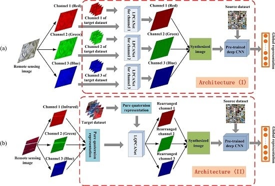
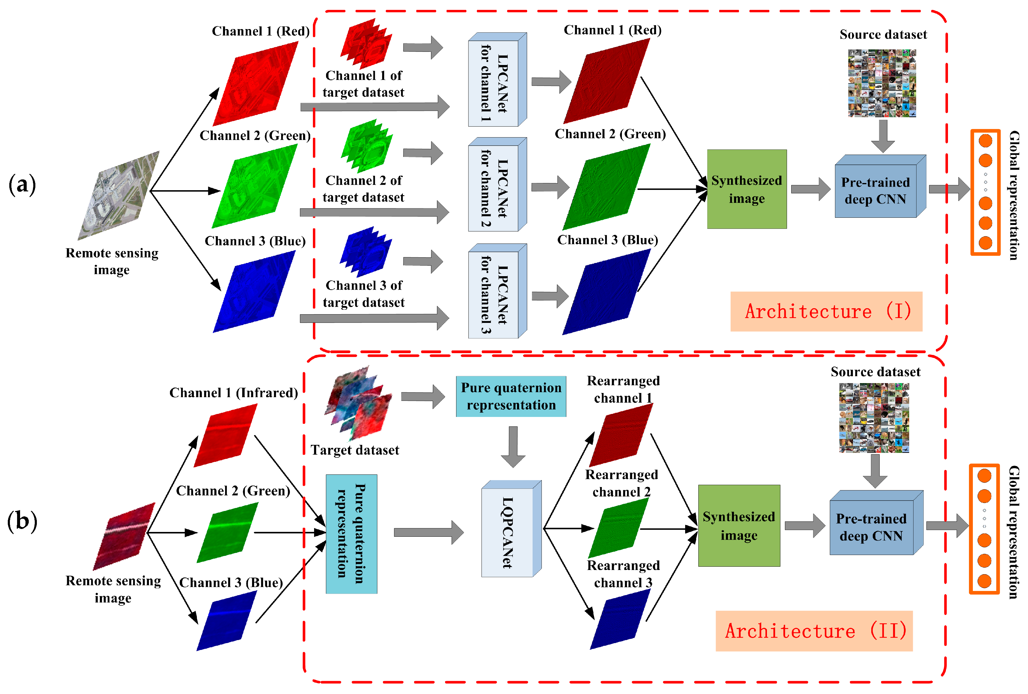
2.3.1. Architecture (I): Synthesizing Spatial Information of Remote Sensing Images to Extract General Features for Pre-Trained Deep CNNs

In Architecture (I), firstly, after dividing the remote sensing image into a series of spectral channels, we apply LPCANet to the “gray” image in each spectral channel. As mentioned in Section 2.2, for remote scene classification task, LPCANet filters out irrelevant details and noise in the remote sensing image, and preserves the main structure of it at the same time. Secondly, for all the spectral channels, the output images of the LPCANets are rearranged into a synthesized image, which is input of the pre-trained deep CNN. By synthesizing spatial information of the remote sensing image, the “distance” between the daily nature image and the remote sensing image is reduced. Then, the pre-trained deep CNN is treated as a fixed feature extractor. In a feedforward way, it extracts a global feature representation of the synthesized image. Finally, with the global representation, we implement remote scene classification by a linear SVM classifier. In addition, we should consider some practical details as following:

• Thus far, almost all successful pre-trained structures of deep CNNs are based on the ImageNet dataset. This results in the constraint that the number of spectral channels of input images should be and only be three when we use the pre-trained deep CNNs to extract global representation from them. This constraint limits the application range of pre-trained deep CNNs and causes inevitable information loss when the number of input images’ spectral channels is more than three.
• Data augmentation is a practical technique to improve the performance of deep CNNs by reducing overfitting in the training stage. However, in this paper, we use the pre-trained deep CNNs in a feedforward way without training on the remote sensing dataset. Because training a deep CNN on a small dataset helps little. Moreover, we usually cannot obtain the labels of remote sensing images in some case. Different from data augmentation, which enhances the generalization power of deep CNNs in supervised framework, LPCANet synthesizes the spatial information of remote sensing images and enhances the generalization power of pre-trained deep CNNs in an unsupervised manner.
• Compared with other remote sensing images such as SAR images, we prefer to apply Architecture (I) to optical remote sensing images. Because the spectral channels of daily natural images in the ImageNet dataset and optical remote sensing images in the target dataset are both red-green-blue, and the “distance” between them is relatively small.

2.3.2. Architecture (II): Further, Synthesizing Spectral Information of Remote Sensing Images to Extract General Features for Pre-Trained Deep CNNs

As discussed above, in the condition that the spectral information of remote sensing images is different from that of images in ImageNet dataset, the “distance” of spectral information between them is relatively large, and the performance of remote scene classification fades evidently when we directly transfer pre-trained deep CNNs to remote scene classification. LPCANet in Architecture (I) can only synthesize spatial information of remote sensing images in each spectral channel. It cannot handle the difference of spectral information between the source and target datasets. Therefore, inspired by quaternion algebra and the relationship of elements in quaternion representation, we represent remote sensing images in quaternion domain, and design the LQPCANet to synthesize spectral information of them. Derive from LPCANet, LQPCANet in Architecture (II) further reduces the “distance” between source dataset and target dataset, and enhances the generalization power of pre-trained deep CNNs for remote scene classification. Firstly, remote sensing images are represented in the form of pure quaternion. Secondly, they are pre-processed by LQPCANet. Then, the synthesized images are put into the pre-trained deep CNN to obtain global feature representation, which is finally used to perform the task of remote scene classification with a linear SVM classifier. The practical details of Architecture (II) are listed as following:

• Considering the constraint of the number of spectral channels that is discussed in Section 2.3.1, we should also obey this constraint in Architecture (II). Because the number of spectral channels of input images is fixed as three, in any case we apply pre-trained deep CNNs to extract global representation from them. Thus, the pure quaternion that contains three imaginary units is used to represent remote sensing images in practice.
• LQPCANet processes the pure quaternion representation of remote sensing images, rearranges the order of their spectral channels, and only maintains the relative relationship of them. Therefore, there is not some distinct spectral channel that we should represent it with some corresponding imaginary unit, when we transform the remote sensing images into pure quaternion form.

3. Experiments and Results

The main objective of this paper is to evaluate the two proposed architectures in enhancing the generalization power of deep pre-trained CNNs for remote scene classification. Therefore, we organize the experiments for Architecture (I) and Architecture (II), respectively, with various deep pre-trained CNNs and various remote sensing datasets.

3.1. Experimental Setup

In this section, we carry out a number of experiments based on Architecture (I) and Architecture (II) respectively. To evaluate their effectiveness in enhancing the generalization power of deep pre-trained CNNs for remote scene classification, we conduct experiments on three remote sensing datasets. These three datasets are different in spatial and spectral information. We compare the performance of our proposed framework with the state-of-the-art results in these three datasets. We must note that except learning the classifier, all the experiments based on Architecture (I) and Architecture (II) are unsupervised.

The three publicly available datasets used in our experiments are as follows:

1

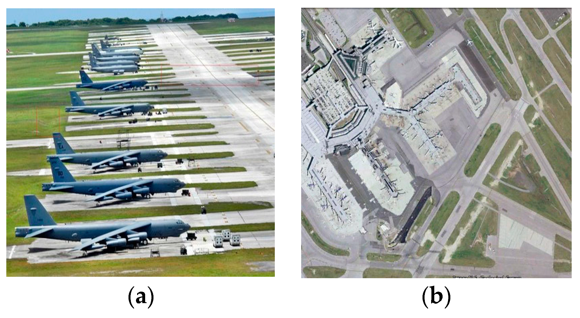
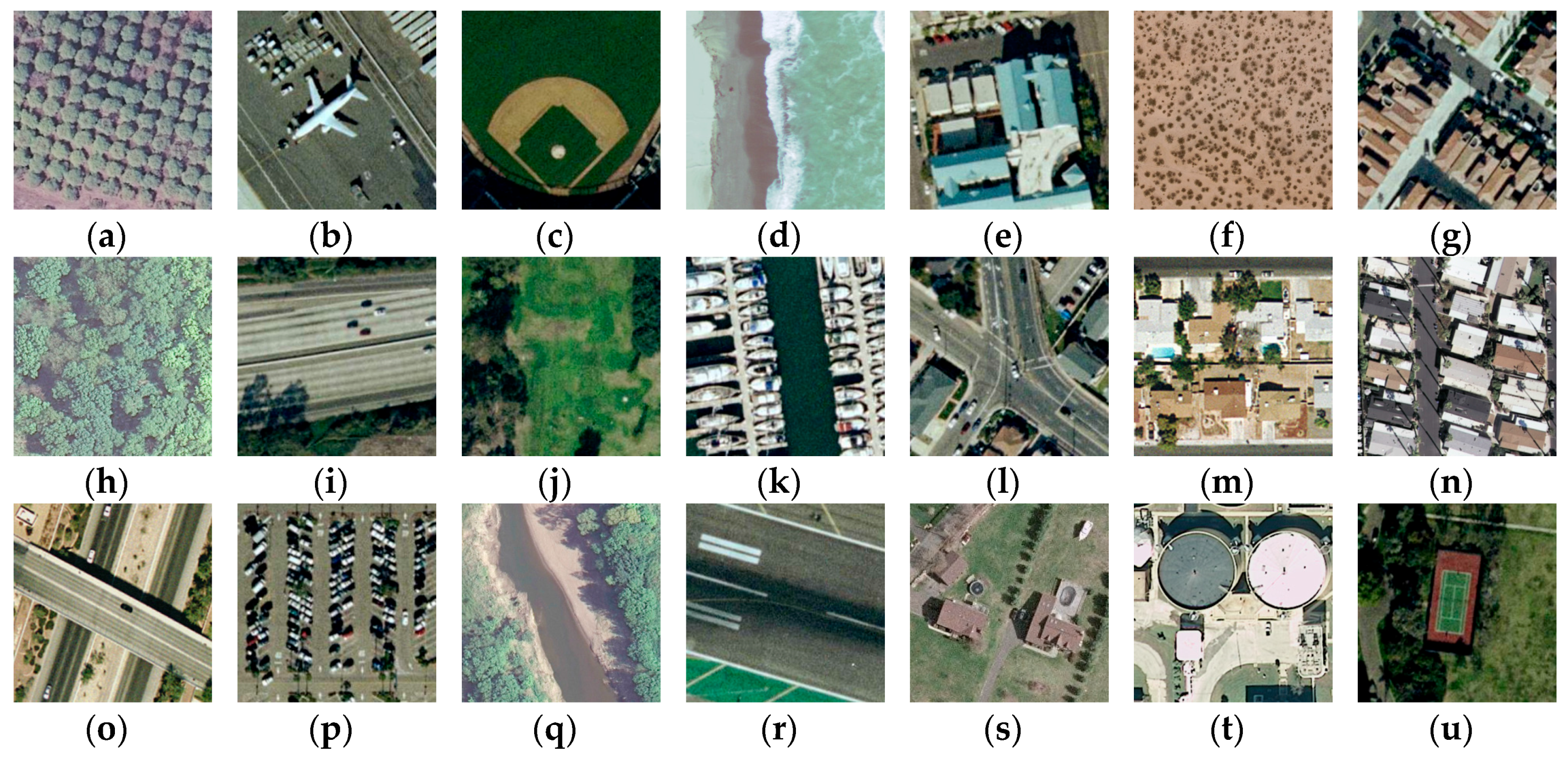
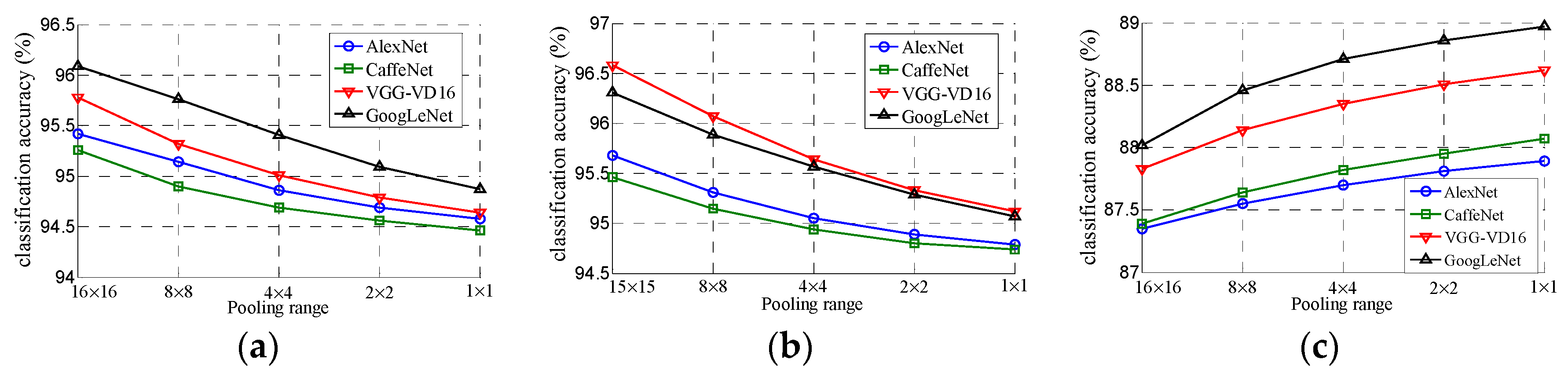
UC Merced Land Use Dataset (http://vision.ucmerced.edu/datasets/landuse.html). Derived from United States Geological Survey (USGS) National Map, this dataset contains 2100 aerial scene images with 256 × 256 pixels, which are manually labeled as 21 land use classes, 100 for each class. Figure 8 shows one example image for each class. As shown in Figure 8, this dataset presents very small inter-class diversity among some categories, such as “dense residential”, “medium residential” and “sparse residential”. More examples and more information are available in [38].

2

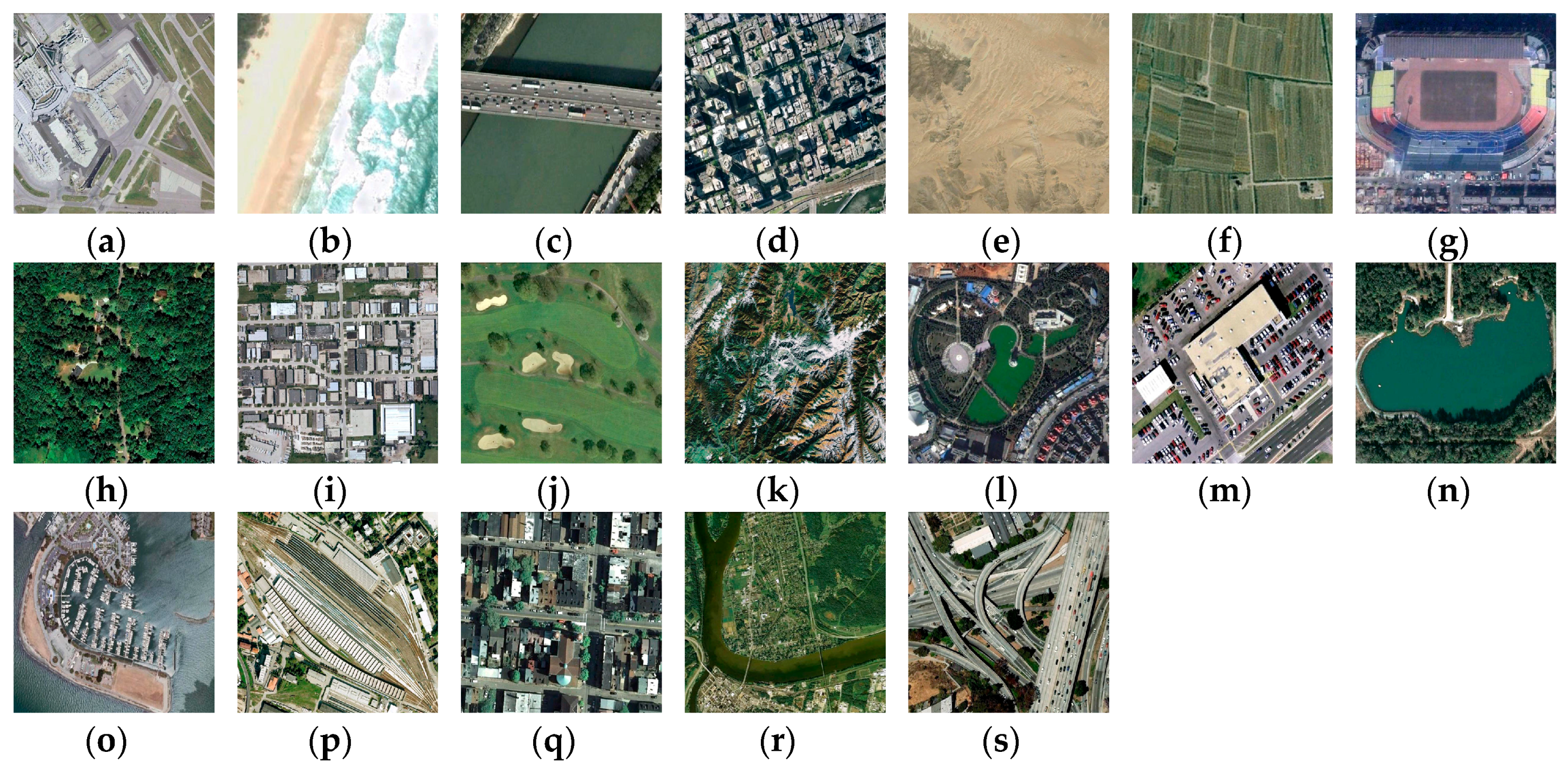
WHU-RS Dataset (http://www.tsi.enst.fr/~xia/satellite_image_project.html). Collected from Google Earth, this dataset is composed of 950 aerial scene images with 600 × 600 pixels, which are uniformly distributed in 19 scene classes, 50 for each class. The example images for each class are shown in Figure 9. We can see that images in both this dataset and UC Merced dataset are optical images (RGB color space). They are same in spectral information. However, compared with the images in UC Merced dataset, images in this dataset contain more detail information in space. The variation of scale and resolution of objects in a wide range within the images makes this dataset more complicated than the UC Merced dataset.

3

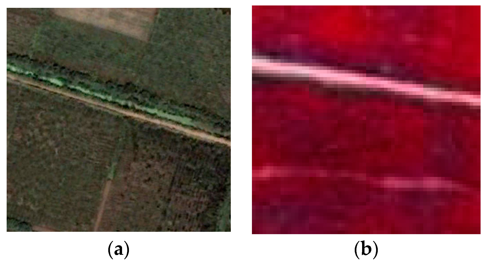
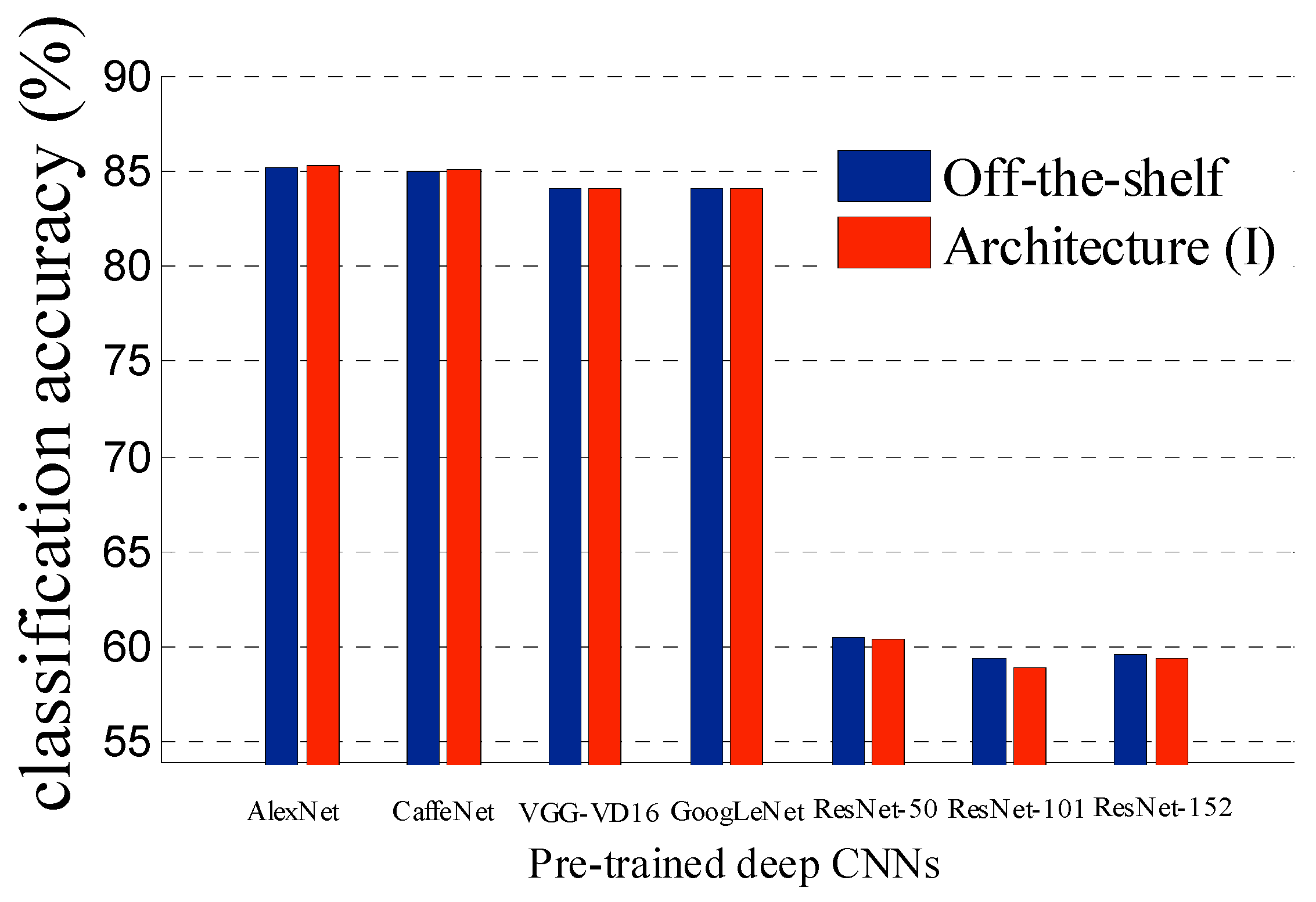
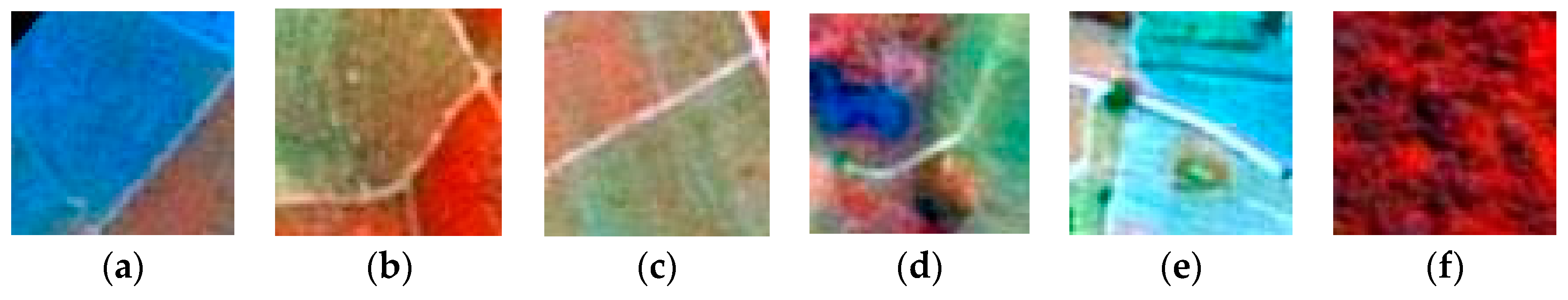
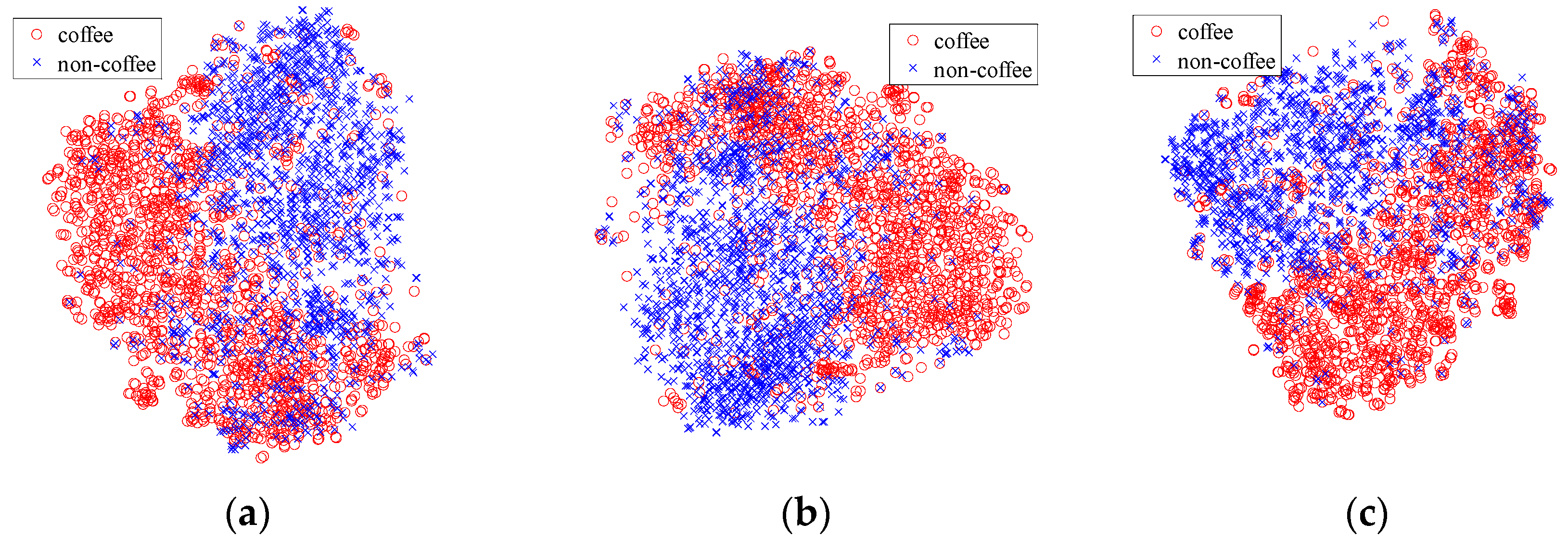
Brazilian Coffee Scenes Dataset (www.patreo.dcc.ufmg.br/downloads/brazilian-coffee-dataset/). Taken by the SPOT sensor in the green, red, and near-infrared bands, over four counties in the State of Minas Gerais, Brazil, this dataset is released in 2015, and includes over 50,000 remote sensing images with 64 × 64 pixels, which are labeled as coffee (1438) non-coffee (36577) or mixed (12989) [25]. Figure 10 shows three example images for each of the coffee and non-coffee classes in false colors. To provide a balanced dataset for the experiments, 1438 images of both coffee and non-coffee classes are picked out, while images of mixed class are all discarded. Note that this dataset is very different from the former two datasets. Images in this dataset are not optical (green–red–infrared instead of red–green–blue).

Following the same experimental protocol of very recent researches [22,25,26], we implement our experiments with five-fold cross-validation. Considering the UC Merced dataset, each of the five folds contains 420 images. As to the WHU-RS dataset, each of the five folds has 190 images. For the Brazilian Coffee Scenes dataset, four folds have 600 images each and the fifth has 476 images. Then, we carry out results in terms of average accuracy and standard deviation among the five folds. On the other hand, we use five well-known pre-trained deep CNNs (AlexNet [15], CaffeNet [17], VGG-VD16 [18], GoogLeNet [28], and ResNet [29]), described in Section 2.1, to test the effectiveness of our proposed Architecture (I) and Architecture (II) in the experiments. As we analyzed before, the operations in both LPCANet (as well as LQPCANet) and pre-trained deep CNN are unsupervised, and all the experiments are in unsupervised framework except learning the classifier.

3.2. Experimental Results of Architecture (I)

We evaluate Architecture (I) in enhancing the generalization power of the five well-known pre-trained deep CNNs for remote scene classification. In Architecture (I), we consider a shallow LPCANet that just has one-stage network. For the LPCANet, we set the PCA filter size as k₁ = k₂ = 8, the number of filters as L = 8, and the pooling range as 8 × 8 without overlapping for local features. The PCA filter banks require that k₁k₂ ≥ L. Note that a larger range for pooling operation provides greater translation invariance in the extracted features $r$. Then, with nearest-neighbor interpolation algorithm, we use the function of “imresize” in Matlab to resize the pooled features map $r$ to 227 × 227 for AlexNet and CaffeNet, and 224 × 224 for VGG-VD16, GoogLeNet and ResNet. Finally, we use a linear SVM as classifier, and implement experiments on the three former proposed remote sensing datasets. These datasets are different in spatial and spectral information in order to test the effectiveness of Architecture (I) in different conditions. Remote sensing images in UC Merced and WHU-RS datasets are both optical. Thus, they are same in spectral information with these images in ImageNet dataset that used to pre-train these deep CNNs. Architecture (I) is mainly designed for this case, and we carry out most experiments for this case. On the other hand, remote sensing images in the Brazilian Coffee Scenes dataset are not optical (green–red–infrared). In this case, the spectral information between source and target datasets is different. We briefly introduce the experiment results of Architecture (I) on this dataset. Architecture (II) is mainly designed for this case, and we will discuss it in Section 3.3 in detail.

With various pre-trained deep CNN models and remote sensing datasets, the remote scene classification performances are shown in

Table 1. Remote scene classification results of five well-known pre-trained deep CNNs on three different remote sensing datasets.

Pre-Trained Deep CNN	UC Merced				WHU-RS				Brazilian Coffee Scenes
	Off-the-Shelf		Architecture (I)		Off-the-Shelf		Architecture (I)		Off-the-Shelf		Architecture (I)
	Ac (%)	SD	Ac (%)	SD	Ac (%)	SD	Ac (%)	SD	Ac (%)	SD	Ac (%)	SD
AlexNet	94.51	0.94	95.43	0.79	94.57	0.61	95.53	0.36	85.14	1.26	85.23	1.13
CaffeNet	94.12	1.05	95.26	0.67	94.67	0.75	95.47	0.69	84.97	1.54	85.12	1.08
VGG-VD16	94.43	0.68	95.59	0.72	94.76	0.72	96.22	0.58	84.12	0.97	84.06	0.84
GoogLeNet	94.57	0.98	95.94	0.59	94.68	1.01	96.14	0.55	84.06	1.16	84.09	0.98
ResNet-50	74.14	5.89	78.32	5.26	75.12	5.36	80.35	5.19	60.54	7.22	60.37	6.93
ResNet-101	72.36	5.96	77.92	5.79	72.85	5.09	78.46	4.48	59.39	6.68	58.92	6.27
ResNet-152	72.48	4.35	77.78	4.13	72.81	4.42	78.52	4.21	59.62	6.81	59.42	6.14

. In Table 1, Ac and SD denote accuracy and standard deviation, respectively. For better comparison, we further show the accuracy of remote scene classification on UC Merced and WHU-RS datasets in Figure 11.

In the condition of Off-the-shelf, pre-trained deep CNNs are directly used as feature extractors in an unsupervised manner. By removing the last fully-connected layer, the rest parts of pre-trained deep CNNs extract high dimensional feature vectors of remote sensing images. These feature vectors are considered as final image representation that followed by a linear SVM classifier. In fact, this framework almost achieves the best performance to date on optical remote sensing datasets [26]. Compared with training deep CNNs with remote sensing images from scratch, transferring pre-trained deep CNNs for remote scene classification shows obvious advantages [22]. Because limited training data of remote sensing dataset brings overfitting seriously, and training from scratch cannot make full use of the deep architecture.

However, in Table 1 and Figure 11, we can see that the performances of AlexNet, CaffeNet, VGG-VD16 and GoogLeNet are almost same. There is obvious bottleneck for directly transferring pre-trained deep CNNs to optical remote scene classification. Moreover, the experiment results overturn our intuition that these CNNs with deeper structure or sophisticated units perform better. In fact, GoogLeNet takes no obvious advantage over AlexNet and CaffeNet, and VGG-VD16 even obtains worse performance than AlexNet. The reason may be that the parameters in deeper layers are more specific for the dataset (ImageNet dataset in this paper) used to pre-train the deep CNNs, and these parameters lack generalization power. In addition, to our surprise, the most successful deep CNNs to date, ResNets fail to obtain a good experiment result, no matter their layers are 50, 101 or 152. This phenomenon indicates that not all successful deep CNNs pre-trained on ImageNet dataset are suitable for transferring to remote scene classification. In ResNets, shortcut connections bring fewer parameters and make the network much easier to optimize. At the same time, the directly connection between input and output brings poor generalization ability when we transfer them for other tasks.

By extracting general features from LPCANet, we propose Architecture (I) to obtain better performance when transferring pre-trained deep CNNs for remote scene classification. As we can see in Table 1 and Figure 11, the remote scene classification accuracy breaks the bottleneck and increases in condition of Architecture (I). Taking a close look into the experiment results, we find that compared with Off-the-shelf, the margin increased by Architecture (I) becomes larger when we apply it to deeper or more sophisticated CNNs such as VGG-VD16 and GoogLeNet. This gives evidence to the conclusion that Architecture (I) can enhance the generalization power of pre-trained deep CNNs and make better use of them. In addition, smaller standard deviation of classification accuracy in condition of Architecture (I) suggests that Architecture (I) is more stable when transferring pre-trained deep CNNs for remote scene classification. Taking pre-trained CaffeNet for example, Figure 12 shows the detail changes of an optical remote sensing image in condition of Off-the-shelf and Architecture (I).

Abbreviated as “conv” and “fc”, reconstructions of convolutional feature maps in the former network layers and that of fully connected layers are shown in Figure 12. Figure 12a shows that the representations of convolutional layers are still photographically similar with the remote sensing image to some extent, although they becomes fuzzier and fuzzier from “conv1” to “conv5”. In addition, the fully connected layers rearrange the information from lower layers to generate representations that are more abstract. They compose of parts (e.g., the wings of airplanes) similar but not identical to the ones found in the original image. In Figure 12b, LPCANet filters out irrelevant details and noise in remote scenes, and preserve the main structure of them at the same time. Based on PCA filters, convolutional operation and weighting operation retain the mainly discrimination ability of remote scenes. On the other hand, the pooling operation enhances the inter-class invariance. As a result, the synthesized image maintains the semantic features of remote scenes with less noise, and become less different with daily optical images in spatial information. Comparing the reconstructed images in fully connected layers in Figure 12a,b, we find that there are more parts in various positions and scales in Figure 12b. Moreover, like wings of airplane, these parts are more discriminative with less blurs. This experiment result further confirms that Architecture (I) can enhance the generalization power of pre-trained deep CNNs and improve their performance for remote sensing images.

To intuitively reflect the distribution of global features learned in condition of Off-the-shelf and Architecture (I), we use the t-SNE algorithm [40,41] to visualize these high-dimensional global features by giving each datapoint a location in a 2-D map. For both conditions, the degree of perplexity and the number of training iterations in the t-SNE algorithm are set as 30 and 1000. We show these 2-D embedding points with different colors corresponding to their actual scene categories. Figure 13 reveals the separability of global features learned by pre-trained CaffeNet when we apply experiment on UC Merced dataset in above two conditions. Notably, the 2-D features from both of the two conditions naturally tend to form clusters. In addition, compared with Off-the shelf, Architecture (I) leads to better separability of global features.

Data augmentation is a practical technique for training an effective deep CNN. However, when we transfer a pre-trained deep CNN for remote scene classification, we treat the pre-trained deep CNN as a fixed feature extractor and do not change the parameters in it. Then, all the extracted features are used to train the classifier. Therefore, data augmentation just affects the classifier, and has no impact on the parameters in pre-trained deep CNNs. For two typical classifiers, we test data augmentation in framework of Architecture (I) on UC Merced dataset by simply rotating the original remote sensing images by 90 degrees, 180 degrees and 270 degrees. We find that the technique of data augmentation indeed works. However, it contributes little as shown in

Table 2. Classification accuracy (%) with and without data augmentation in framework of Architecture (I) on UC Merced dataset.

Pre-Trained Deep CNN	Linear SVM		Softmax
	With Aug	Without Aug	With Aug	Without Aug
AlexNet	95.85	95.43	96.01	95.78
CaffeNet	95.81	95.26	96.08	95.74
VGG-VD16	96.15	95.59	96.26	95.90
GoogLeNet	96.67	95.94	96.95	96.03
ResNet-50	79.22	78.32	79.54	78.58
ResNet-101	78.64	77.92	79.52	78.65
ResNet-152	78.83	77.78	79.30	78.59

.

To further verify the effectiveness of LPCANet in Architecture (I), in Figure 14, we directly apply PCA algorithm to every single image in UC Merced dataset before the block of pre-trained deep CNN. This simple architecture, called Architecture (S), is designed for comparison. Without augmentation,

Table 3. Classification accuracy (%) of Architecture (S), Architecture (I) and Off-the-shelf on UC Merced dataset.

Pre-Trained Deep CNN	Architecture (S)	Architecture (I)	off-the-Shelf
AlexNet	92.25	95.43	94.51
CaffeNet	92.37	95.26	94.12
VGG-VD16	92.71	95.59	94.43
GoogLeNet	93.16	95.94	94.57
ResNet-50	72.85	78.32	74.14
ResNet-101	70.79	77.92	72.36
ResNet-152	70.92	77.78	72.48

shows the experiment results on UC Merced dataset. We can see that the classification accuracy fades in condition of Architecture (S) compared with the conditions of Architecture (I) and Off-the-shelf. This gives evidence that simply applying PCA algorithm to remote sensing images may lose some discriminative spatial information, and cannot obtain general features for pre-trained deep CNNs. The experiment results further confirm the effectiveness of our proposed Architecture (I).

Various state-of-the-art methods have been proposed recently for remote scene classification, and most of them have been tested on the UC Merced dataset, following the same experimental protocol, with five-fold cross validation. Thus, in

Table 4. Classification accuracy (%) of reference and proposed methods on the UC Merced dataset.

Method	Year	Reference	Accuracy
SCK	2010	[38]	72.52
SPCK++	2011	[42]	77.38
BRSP	2012	[43]	77.80
UFL	2014	[5]	81.67
CCM-BOVW	2014	[11]	86.64
mCENTRIST	2014	[44]	89.90
MSIFT	2014	[45]	90.97
COPD	2014	[46]	91.33
Dirichlet	2014	[47]	92.80
VLAT	2014	[13]	94.30
MCMI-based	2015	[48]	88.20
PSR	2015	[12]	89.10
UFL-SC	2015	[49]	90.26
Partlets	2015	[50]	91.33
Sparselets	2015	[51]	91.46
Pre-trained CaffeNet	2015	[25]	93.42
FBC	2016	[52]	85.53
LPCNN	2016	[53]	89.90
MTJSLRC	2016	[54]	91.07
SSBFC	2016	[55]	91.67
CTS	2016	[56]	93.08
SRSCNN	2016	[57]	95.10
LGF	2016	[58]	95.48
Architecture (I)	—	—	96.95

we compare our best result achieved via Architecture (I) with these methods on the UC Merced dataset. With straightforward and simple framework, our proposed Architecture (I) outperforms all the methods with a minimum gap of almost 1.5%. We must note that our proposed method just provides basic framework to directly transfer pre-trained deep CNNs for remote scene classification in an unsupervised manner, and do not use target dataset to train the parameters in the pre-trained CNNs. Therefore, our proposed method achieves no better result than the GoogLeNet + Fine-tune approach in [22]. The effectiveness of fine-tuning approach is much dependent on the amount of images in remote sensing dataset, and the computation time of it is more demanding compared with our proposed Architecture (I). In fact, in Table 1, we can see that, with pre-trained CaffeNet in Architecture (I), the experiment result on UC Merced dataset has almost achieved the performance of fine-tuning approach in [22]. In addition, if the task of remote scene classification permits sufficient computation time, with sufficient remote sensing images, we can further fine-tune the parameters of pre-trained deep CNNs in Architecture (I).

In the Brazilian Coffee Scenes dataset, remote sensing images are not optical (green–red–infrared). In addition, as shown in Figure 10, the spatial information of these images is very simple. In Table 1, the relatively poor performance comes from the difference in spectral information when we transferring pre-trained deep CNNs to remote scene classification on this dataset. As we analyzed before, LPCANet in Architecture (I) changes no spectral information of remote sensing images. In addition, when spatial information of remote sensing images is simple, the effect of LPCANet in Architecture (I) is weakened in decreasing the “distance” between target dataset and source dataset. For this dataset, experiment results in Figure 15 indicate that Architecture (I) helps little and even make things worse when the spectral information of remote sensing images is very different from these images in source dataset.

3.3. Experimental Results of Architecture (II)

As discussed before, Architecture (I) obtains poor performance on Brazilian Coffee Scenes dataset, in which the spectral information of remote sensing images is very different from that of images in ImageNet dataset used to pre-train the deep CNNs. Therefore, we propose Architecture (II) to handle the difference of spectral information between source and target datasets, and further enhance the generalization power of pre-trained deep CNNs for remote scene classification. With the same experiment parameters in Section 3.2, we report remote scene classification results in

Table 5. Classification accuracy (%) of Architecture (II), Architecture (I) and Off-the-shelf on different remote sensing datasets.

Pre-Trained Deep CNN	UC Merced			WHU-RS			Brazilian Coffee Scenes
	Ar(II)	Ar(I)	OTS	Ar(II)	Ar(I)	OTS	Ar(II)	Ar(I)	OTS
AlexNet	95.14	95.43	94.51	95.31	95.53	94.57	87.55	85.23	85.14
CaffeNet	94.90	95.26	94.12	95.15	95.47	94.67	87.64	85.12	84.97
VGG-VD16	95.32	95.59	94.43	96.07	96.22	94.76	88.14	84.06	84.12
GoogLeNet	95.76	95.94	94.57	95.89	96.14	94.68	88.46	84.09	84.06
ResNet-50	77.06	78.32	74.14	79.15	80.35	75.12	68.85	60.37	60.54
ResNet-101	76.65	77.92	72.36	78.38	78.46	72.85	68.26	58.92	59.39
ResNet-152	76.89	77.78	72.48	78.10	78.52	72.81	68.44	59.42	59.62

for Architecture (II), Architecture (I) and Off-the-shelf on the three proposed remote sensing datasets.

In Table 5, Ar(II), Ar(I) and OTS denote Architecture (II), Architecture (I) and Off-the-shelf respectively. From the experiment results, we find that Architecture (II) is superior to Architecture (I) and Off-the-shelf with a substantial gain on Brazilian Coffee Scenes dataset for all the pre-trained deep CNNs. On the other hand, Architecture (II) is slightly inferior to Architecture (I) on the UC Merced and WHU-RS datasets. Nevertheless, the remote scene classification accuracy of Architecture (II) is higher than that of Off-the-shelf in any case. These experiment results confirm what we discussed in Section 2.3.2. LQPCANet in Architecture (II) rearranges the spectral information of remote sensing images in Brazilian Coffee Scenes dataset and reduce the “distance” between source dataset and target dataset in the transferring process. As a result, Architecture (II) makes better use of the high-level features in pre-trained deep CNNs and enhances their generalization power when the spectral information is different between source and target datasets.

Taking a close look into Figure 10, we observe that remote sensing images in Brazilian Coffee Scenes dataset are composed of simple edges. Namely, the spatial information of these images is very simple, and we should pay more attention to the discrimination of inter-class variability instead of the invariance of intra-class variability. On the contrary, as shown in Figure 8 and Figure 9, the invariance of intra-class variability is more important for remote scene classification on UC Merced and WHU-RS datasets. Therefore, we further test the effectiveness of pooling operation in LQPCANet in Architecture (II). With different pooling ranges in Architecture (II), the remote scene classification accuracies on different datasets are reported in Figure 16. These pooling ranges are set according to the size of images in specific remote sensing dataset to guarantee the non-overlapping pooling operation. In addition, when we apply different pooling ranges in the experiments, the difference of classification accuracies is not obvious. Thus, in the condition of each pooling range, we iterate the experiment 10 times and show the average result in Figure 16.

Figure 16 shows that the pooling range in LQPCANet may affect the performance of Architecture (II). When the remote sensing images are composed of sophisticated objects, a relatively larger pooling range in Architecture (II) enhances the invariance of intra-class variability and brings better performance in remote scene classification. On the contrary, a relatively smaller pooling range contributes more when the remote sensing images consist of simple edges or blobs such as images in Brazilian Coffee Scenes dataset. Moreover, inspired by Figure 16, we may prefer to design a relatively larger pooling range in the LPCANet when we apply Architecture (I) to UC Merced and WHU-RS datasets in Section 3.2.

Furthermore, we visualize the global representations of remote sensing images in Brazilian Coffee Scenes dataset. These global representations are encoded via pre-trained CaffeNet in Architecture (II), Architecture (I) and Off-the-shelf respectively. High-dimensional image features are embedded on a 2-D space by using the t-SNE algorithm [40,41]. For all conditions, the degree of perplexity and the number of training iterations in t-SNE algorithm are set as 30 and 1000. As shown in Figure 17, with same pre-trained deep CNN, Architecture (II) leads to the best separability of global representations in the case that spectral information is different between source and target datasets. As a result, Architecture (II) enhances the generalization power of pre-trained deep CNN and brings better performance for remote scene classification on Brazilian Coffee Scenes dataset.

On the Brazilian Coffee Scenes dataset, we further compare the performance of Architecture (II) with several well-known methods. The comparison is relatively insufficient as shown in

Table 6. Classification accuracy (%) of reference and proposed methods on the Brazilian Coffee Scenes dataset.

Method	Year	Reference	Accuracy
BIC	2015	[25]	87.03
BOVW	2015	[22]	80.50
Pre-trained CaffeNet	2015	[22]	85.02
Pre-trained GoogLeNet	2015	[22]	84.02
Architecture (II)	—	—	88.46

. Because this dataset is newly released in 2015 [25], and there are not sufficient researches on it. We find that our proposed Architecture (II) performs well without training or fine-tuning the parameters in pre-trained CNNs. In [22], training deep CNNs from scratch with Brazilian Coffee Scenes dataset achieves classification accuracy up to 91.83%. However, training a deep CNN from scratch is very time-consuming and this depend much on the scale of target dataset. Comparing the method of directly transferring pre-trained GoogLeNet for remote scene classification (84.02%) with Architecture (II) that contains the same pre-trained GoogLeNet (88.46%), we give evidence that Architecture (II) indeed enhances the generalization power of pre-trained CNNs for remote scene classification when the spectral information is different between source and target datasets.

4. Discussion

From the extensive experiments above, our two proposed architectures, which contain LPCANet and LQPCANet, respectively, have been proven to be effective for remote scene classification. As discussed in [22,25,26], deep CNNs pre-trained on everyday objects can be successfully transferred to remote sensing domain. To some degree, this transferring strategy achieves the state-of-the-art performance for remote scene classification. The major factor that affects this transferring process is proven to be the generalization power of pre-trained deep CNNs [59,60,61]. However, the difference of spatial and spectral information between source and target datasets brings bottleneck for the generalization power of pre-trained deep CNNs as shown in our experiments. Based on transferring pre-trained deep CNNs, Castelluccio et al. [22,25] further improve the performance of remote scene classification by fine-tuning and feature fusing respectively. Nevertheless, they do no efforts about the remote sensing images for the transferring process. In our proposed Architecture (I), the LPCANet is used to filter out noise and enhance the edges in remote sensing images. On the other hand, LQPCANet in Architecture (II) further rearranges the relative relationship of spectral channels for remote sensing images. The two proposed architectures in our paper enhance the generalization power of pre-trained deep CNNs for remote scene classification and break the bottleneck mentioned above. Moreover, our method can be seen as a starting point, and be further improved by fine-tuning or feature fusing. Specifically, several practical observations from the experiments and some limitations of our study are summarized as follows:

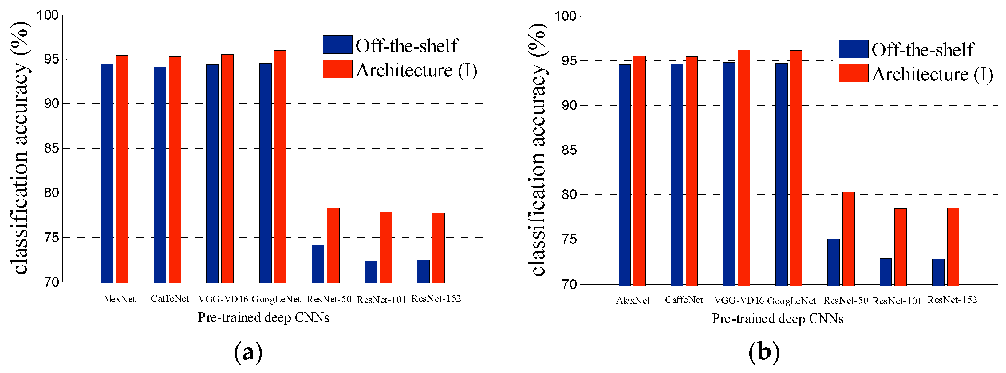
• In Table 1 and Table 5, we can see that the performances of pre-trained AlexNet, CaffeNet, VGG-VD16 and GoogLeNet are almost same in remote scene classification in condition of Off-the-shelf. There is obvious bottleneck for directly transferring pre-trained deep CNNs to the task of remote scene classification. Our proposed two architectures improve the performance of pre-trained CNNs in an unsupervised manner and provide a better starting point for further method (such as fine-tuning and feature fusing) to get better performance for remote scene classification.
• To our surprise, the most successful deep CNNs to date, ResNets, fail to obtain good experiment result when we transfer it for remote scene classification, no matter their layers are 50, 101 or 152. This phenomenon indicates that not all successful deep CNNs are suitable for transferring to the task of remote scene classification.
• The selection of our two proposed architectures depends on the target dataset in the transferring process, namely the remote sensing dataset when we transfer pre-trained deep CNNs for remote scene classification. When the spectral information of source and target datasets are the same, we use Architecture (I), and we prefer to Architecture (II) when their spectral information is different.
• Compared with directly transferring pre-trained deep CNNs for remote scene classification, our method provides a new way to optimize the transferring process. When we transfer any successful deep CNN explored in future for remote scene classification, we can make it a step further with our proposed method.
• The transferring strategy in our paper is limited by the spectral channels of input images for the deep CNNs pre-trained by everyday optical images. For remote sensing images whose spectral channels are more than three, their spectral dimensions must be reduces to three to fit the pre-trained deep CNNs transferred to them. With no doubt, this operation brings spectral information loss.
• In the remote sensing field, the scale of remote sensing datasets will be larger and larger. On the other hand, the structure of deep CNN will be optimized, and the parameters in it will be less and less. Therefore, in our proposed framework we could get more and more useful information from remote sensing datasets, obtain better generalization power of pre-trained deep CNNs and run into less overfitting.

Based on our study, the future research directions of transferring pre-trained deep CNNs for remote scene classification may be as follows. Firstly, different from empirically choosing parameters in LPCANet and LQPCANet in this paper, how to regulate their parameters to obtain better performance remains to be learned. Secondly, instead of placing LPCANet or LQPCANet before pre-trained deep CNNs, would replacing some convolutional layers in pre-trained deep CNNs with LPCANet or LQPCANet work? Finally, as we discussed above, when transferring the most successful ResNet for remote scene classification, it does not works as we expected. Thus, we should find the proper structure of deep CNNs that are more suitable to transfer to remote sensing field.

5. Conclusions

In this paper, we have presented a framework to enhance the generalization power of pre-trained deep CNNs for remote scene classification. To handle the difference of spatial and spectral information between remote sensing images and images in pre-training dataset, two promising architectures are proposed to reduce the “distance” between them.

The two main conclusions of this work are that: (1) For the difference in spatial information between remote sensing dataset and pre-training dataset, Architecture (I) enhances the generalization power of pre-trained deep CNNs in it and achieve better performance in remote scene classification. Linear PCA network in Architecture (I) synthesize spatial information of remote sensing images in each spectral channel, and reduces the spatial “distance” between source and target datasets; (2) When remote sensing dataset and the source dataset are different in spectral information, remote sensing images are represented as pure quaternion in linear quaternion PCA network, which further synthesizes spectral information of them. As a result, Architecture (II) enhances the generalization power of the pre-trained deep CNN in it, and improves the classification accuracy of remote scenes. Experiments on three datasets with different properties have provided insightful information. Architecture (I) outperforms the Off-the-shelf method with a gain up to 1.37% on UC Merced dataset and 1.46% on WHU-RS dataset. Architecture (II) outperforms the Off-the-shelf method with a gain up to 4.4% on Brazilian Coffee Scenes dataset. Moreover, the effect of our proposed architectures becomes more evident when the “distance” between source and target datasets becomes larger.

We believe our proposed method in this work can serve as a good baseline for people to transfer pre-trained deep CNNs to other remote sensing datasets with more advanced processing components or more sophisticated structures.

References

1. Wang, J.; Qin, Q.; Li, Z.; Ye, X.; Wang, J.; Yang, X.; Qin, X. Deep hierarchical representation and segmentation of high resolution remote sensing images. In Proceedings of the 2015 IEEE International Geoscience and Remote Sensing Symposium, Milan, Italy, 26–31 July 2015; pp. 4320–4323.
2. Nijim, M.; Chennuboyina, R.D.; Al Aqqad, W. A supervised learning data mining approach for object recognition and classification in high resolution satellite data. World Acad. Sci. Eng. Technol. Int. J. Comput. Electr. Autom. Control Inf. Eng. 2015, 9, 2472–2476. [Google Scholar]
3. Vakalopoulou, M.; Karantzalos, K.; Komodakis, N.; Paragios, N. Building detection in very high resolution multispectral data with deep learning features. In Proceedings of the 2015 IEEE International Geoscience and Remote Sensing Symposium, Milan, Italy, 26–31 July 2015; pp. 1873–1876.
4. Zhou, W.; Shao, Z.; Diao, C.; Cheng, Q. High-resolution remote-sensing imagery retrieval using sparse features by auto-encoder. Remote Sens. Lett. 2015, 6, 775–783. [Google Scholar] [CrossRef]
5. Cheriyadat, A.M. Unsupervised feature learning for aerial scene classification. IEEE Trans. Geosci. Remote Sens. 2014, 52, 439–451. [Google Scholar] [CrossRef]
6. Xu, Y.; Huang, B. Spatial and temporal classification of synthetic satellite imagery: Land cover mapping and accuracy validation. Geo-Spat. Inf. Sci. 2014, 17, 1–7. [Google Scholar] [CrossRef]
7. Yang, W.; Yin, X.; Xia, G.S. Learning high-level features for satellite image classification with limited labeled samples. IEEE Trans. Geosci. Remote Sens. 2015, 53, 4472–4482. [Google Scholar] [CrossRef]
8. Shao, W.; Yang, W.; Xia, G.S. Extreme value theory-based calibration for the fusion of multiple features in high-resolution satellite scene classification. Int. J. Remote Sens. 2013, 34, 8588–8602. [Google Scholar] [CrossRef]
9. Romero, A.; Gatta, C.; Camps-Valls, G. Unsupervised deep feature extraction for remote sensing image classification. IEEE Trans. Geosci. Remote Sens. 2016, 54, 1349–1362. [Google Scholar] [CrossRef]
10. Lazebnik, S.; Schmid, C.; Ponce, J. Beyond bags of features: Spatial pyramid matching for recognizing natural scene categories. In Proceedings of the 2006 IEEE Computer Society Conference on Computer Vision and Pattern Recognition, New York, NY, USA, 17–22 June 2006; Volume 2, pp. 2169–2178.
11. Zhao, L.J.; Tang, P.; Huo, L.Z. Land-use scene classification using a concentric circle-structured multiscale bag-of-visual-words model. IEEE J. Sel. Top. Appl. Earth Obs. Remote Sens. 2014, 7, 4620–4631. [Google Scholar] [CrossRef]
12. Chen, S.; Tian, Y.L. Pyramid of spatial relatons for scene-level land use classification. IEEE Trans. Geosci. Remote Sens. 2015, 53, 1947–1957. [Google Scholar] [CrossRef]
13. Negrel, R.; Picard, D.; Gosselin, P.H. Evaluation of second-order visual features for land-use classification. In Proceedings of the IEEE 12th International Workshop on Content-Based Multimedia Indexing, Klagenfurt, Austria, 18–20 June 2014; pp. 1–5.
14. LeCun, Y.; Bottou, L.; Bengio, Y.; Haffner, P. Gradient-based learning applied to document recognition. Proc. IEEE 1998, 86, 2278–2324. [Google Scholar] [CrossRef]
15. Krizhevsky, A.; Sutskever, I.; Hinton, G.E. Imagenet classification with deep convolutional neural networks. In Proceedings of the Advances in Neural Information Processing Systems, Lake Tahoe, NV, USA, 3–8 December 2012; pp. 1097–1105.
16. Sermanet, P.; Eigen, D.; Zhang, X.; Mathieu, M.; Fergus, R.; LeCun, Y. Overfeat: Integrated recognition, localization and detection using convolutional networks. arXiv, 2013; arXiv:1312.6229. [Google Scholar]
17. Jia, Y.; Shelhamer, E.; Donahue, J.; Karayev, S.; Long, J.; Girshick, R.; Darrell, T. Caffe: Convolutional architecture for fast feature embedding. In Proceedings of the 22nd ACM International Conference on Multimedia, Orlando, FL, USA, 3–7 November 2014; pp. 675–678.
18. Simonyan, K.; Zisserman, A. Very deep convolutional networks for large-scale image recognition. arXiv, 2014; arXiv:1409.1556. [Google Scholar]
19. Hu, W.; Huang, Y.; Wei, L.; Zhang, F.; Li, H. Deep convolutional neural networks for hyperspectral image classification. J. Sens. 2015. [Google Scholar] [CrossRef]
20. Makantasis, K.; Karantzalos, K.; Doulamis, A.; Doulamis, N. Deep supervised learning for hyperspectral data classification through convolutional neural networks. In Proceedings of the 2015 IEEE International Geoscience and Remote Sensing Symposium, Milan, Italy, 26–31 July 2015; pp. 4959–4962.
21. Hamida, A.B.; Benoit, A.; Lambert, P.; Ben, A.C. Deep learning approach for remote sensing image analysis. In Proceedings of the Big Data from Space, Santa Cruz De Tenerife, Spain, 15–17 March 2016; p. 133.
22. Castelluccio, M.; Poggi, G.; Sansone, C.; Verdoliva, L. Land use classification in remote sensing images by convolutional neural networks. arXiv, 2015; arXiv:1508.00092. [Google Scholar]
23. Deng, J.; Dong, W.; Socher, R.; Li, L.J.; Li, K.; Li, F.F. Imagenet: A large-scale hierarchical image database. In Proceedings of the 2009 IEEE Conference on Computer Vision and Pattern Recognition, Miami, FL, USA, 20–29 June 2009; pp. 248–255.
24. Nanni, L.; Ghidoni, S. How could a subcellular image, or a painting by Van Gogh, be similar to a great white shark or to a pizza? Pattern Recognit. Lett. 2017, 85, 1–7. [Google Scholar] [CrossRef]
25. Penatti, O.A.B.; Nogueira, K.; dos Santos, J.A. Do deep features generalize from everyday objects to remote sensing and aerial scenes domains? In Proceedings of the IEEE Conference on Computer Vision and Pattern Recognition Workshops, Boston, MA, USA, 7–12 July 2015; pp. 44–51.
26. Hu, F.; Xia, G.S.; Hu, J.; Zhang, L. Transferring deep convolutional neural networks for the scene classification of high-resolution remote sensing imagery. Remote Sens. 2015, 7, 14680–14707. [Google Scholar] [CrossRef]
27. Chan, T.H.; Jia, K.; Gao, S.; Lu, J.; Zeng, Z.; Ma, Y. PCANet: A simple deep learning baseline for image classification? IEEE Trans. Image Process. 2015, 24, 5017–5032. [Google Scholar] [CrossRef] [PubMed]
28. Szegedy, C.; Liu, W.; Jia, Y.; Sermanet, P.; Reed, S.; Anguelov, D.; Erhan, D.; Vanhoucke, A.; Rabinovich, A. Going deeper with convolutions. In Proceedings of the IEEE Conference on Computer Vision and Pattern Recognition, Boston, MA, USA, 7–12 July 2015; pp. 1–19.
29. He, K.; Zhang, X.; Ren, S.; Sun, J. Deep residual learning for image recognition. arXiv, 2015; arXiv:1512.03385. [Google Scholar]
30. Hubel, D.H.; Wiesel, T.N. Receptive fields of single neurones in the cat’s striate cortex. J. Physiol. 1959, 148, 574–591. [Google Scholar] [CrossRef] [PubMed]
31. Fukushima, K. Neocognitron: A self-organizing neural network model for a mechanism of pattern recognition unaffected by shift in position. Biol. Cybern. 1980, 36, 193–202. [Google Scholar] [CrossRef] [PubMed]
32. LeCun, Y.; Boser, B.; Denker, J.S.; Henderson, D.; Howard, R.E.; Hubbard, W.; Jackel, L.D. Backpropagation applied to handwritten zip code recognition. Neural Comput. 1989, 1, 541–551. [Google Scholar] [CrossRef]
33. Russakovsky, O.; Deng, J.; Su, H.; Krause, J.; Satheesh, S.; Ma, S.; Huang, Z.; Karpathy, A.; Khosla, A.; Bernstein, M.; et al. Imagenet large scale visual recognition challenge. Int. J. Comput. Vis. 2015, 115, 211–252. [Google Scholar] [CrossRef]
34. He, K.; Sun, J. Convolutional neural networks at constrained time cost. In Proceedings of the IEEE Conference on Computer Vision and Pattern Recognition, Boston, MA, USA, 7–12 July 2015; pp. 5353–5360.
35. Lin, M.; Chen, Q.; Yan, S. Network in network. arXiv, 2013; arXiv:1312.4400. [Google Scholar]
36. Szegedy, C.; Vanhoucke, V.; Ioffe, S.; Shlens, J.; Wojna, Z. Rethinking the inception architecture for computer vision. arXiv, 2015; arXiv:1512.00567. [Google Scholar]
37. Szegedy, C.; Ioffe, S.; Vanhoucke, V. Inception-v4, inception-resnet and the impact of residual connections on learning. arXiv, 2016; arXiv:1602.07261. [Google Scholar]
38. Yang, Y.; Newsam, S. Bag-of-visual-words and spatial extensions for land-use classification. In Proceedings of the 18th SIGSPATIAL International Conference on Advances in Geographic Information Systems, San Jose, CA, USA, 2–5 November 2010; pp. 270–279.
39. Mahendran, A.; Vedaldi, A. Understanding deep image representations by inverting them. In Proceedings of the 2015 IEEE Conference on Computer Vision and Pattern Recognition (CVPR), Boston, MA, USA, 7–12 July 2015; pp. 5188–5196.
40. Maaten, L.; Hinton, G. Visualizing data using t-SNE. J. Mach. Learn. Res. 2008, 9, 2579–2605. [Google Scholar]
41. Van der Maaten, L. Accelerating t-SNE using tree-based algorithms. J. Mach. Learn. Res. 2014, 15, 3221–3245. [Google Scholar]
42. Yang, Y.; Newsam, S. Spatial pyramid co-occurrence for image classification. In Proceedings of the IEEE 2011 International Conference on Computer Vision, Providence, RI, USA, 20–25 June 2011; pp. 1465–1472.
43. Jiang, Y.; Yuan, J.; Yu, G. Randomized spatial partition for scene recognition. In Computer Vision–ECCV 2012; Springer: Berlin/Heidelberg, Germany, 2012; pp. 730–743. [Google Scholar]
44. Xiao, Y.; Wu, J.; Yuan, J. mCENTRIST: A multi-channel feature generation mechanism for scene categorization. IEEE Trans. Image Process. 2014, 23, 823–836. [Google Scholar] [CrossRef] [PubMed]
45. Avramović, A.; Risojević, V. Block-based semantic classification of high-resolution multispectral aerial images. Signal Image Video Process. 2016, 10, 75–84. [Google Scholar] [CrossRef]
46. Cheng, G.; Han, J.; Zhou, P.; Guo, L. Multi-class geospatial object detection and geographic image classification based on collection of part detectors. ISPRS J. Photogramm. Remote Sens. 2014, 98, 119–132. [Google Scholar] [CrossRef]
47. Kobayashi, T. Dirichlet-based histogram feature transform for image classification. In Proceedings of the IEEE Conference on Computer Vision and Pattern Recognition, Columbus, OH, USA, 23–28 June 2014; pp. 3278–3285.
48. Ren, J.; Jiang, X.; Yuan, J. Learning LBP structure by maximizing the conditional mutual information. Pattern Recognit. 2015, 48, 3180–3190. [Google Scholar] [CrossRef]
49. Hu, F.; Xia, G.S.; Wang, Z.; Huang, X.; Zhang, L.; Sun, H. Unsupervised feature learning via spectral clustering of multidimensional patches for remotely sensed scene classification. IEEE J. Sel. Top. Appl. Earth Obs. Remote Sens. 2015, 8, 2015–2030. [Google Scholar] [CrossRef]
50. Cheng, G.; Han, J.; Guo, L.; Liu, Z.; Bu, S.; Ren, J. Effective and efficient midlevel visual elements-oriented land-use classification using VHR remote sensing images. IEEE Trans. Geosci. Remote Sens. 2015, 53, 4238–4249. [Google Scholar] [CrossRef]
51. Cheng, G.; Han, J.; Guo, L.; Liu, T. Learning coarse-to-fine sparselets for efficient object detection and scene classification. In Proceedings of the IEEE Conference on Computer Vision and Pattern Recognition, Boston, MA, USA, 7–12 June 2015; pp. 1173–1181.
52. Hu, F.; Xia, G.S.; Hu, J.; Zhong, Y.; Xu, K. Fast binary coding for the scene classification of high-resolution remote sensing imagery. Remote Sens. 2016, 8, 555. [Google Scholar] [CrossRef]
53. Zhong, Y.; Fei, F.; Zhang, L. Large patch convolutional neural networks for the scene classification of high spatial resolution imagery. J. Appl. Remote Sens. 2016, 10, 025006. [Google Scholar] [CrossRef]
54. Qi, K.; Liu, W.; Yang, C.; Guan, Q.; Wu, H. High Resolution Satellite Image Classification Using Multi-Task Joint Sparse and Low-Rank Representation; Preprints: Basel, Switzerland, 2016. [Google Scholar]
55. Zhao, B.; Zhong, Y.; Zhang, L. A spectral–structural bag-of-features scene classifier for very high spatial resolution remote sensing imagery. ISPRS J. Photogramm. Remote Sens. 2016, 116, 73–85. [Google Scholar] [CrossRef]
56. Yu, H.; Yang, W.; Xia, G.S.; Liu, G. A Color-Texture-structure descriptor for high-resolution satellite image classification. Remote Sens. 2016, 8, 259. [Google Scholar] [CrossRef]
57. Liu, Y.; Zhong, Y.; Fei, F.; Zhang, L. Scene semantic classification based on random-scale stretched convolutional neural network for high-spatial resolution remote sensing imagery. In Proceedings of the IEEE International Geoscience and Remote Sensing Symposium, Beijing, China, 10–15 July 2016; pp. 763–766.
58. Zou, J.; Li, W.; Chen, C.; Du, Q. Scene classification using local and global features with collaborative representation fusion. Inf. Sci. 2016, 348, 209–226. [Google Scholar] [CrossRef]
59. Sharif Razavian, A.; Azizpour, H.; Sullivan, J.; Carlsson, S. CNN features off-the-shelf: An astounding baseline for recognition. In Proceedings of the IEEE Conference on Computer Vision and Pattern Recognition Workshops, Columbus, OH, USA, 23–28 June 2014; pp. 806–813.
60. Girshick, R.; Donahue, J.; Darrell, T.; Malik, J. Rich feature hierarchies for accurate object detection and semantic segmentation. In Proceedings of the IEEE Conference on Computer Vision and Pattern Recognition, Columbus, OH, USA, 24–27 June 2014; pp. 580–587.
61. He, K.; Zhang, X.; Ren, S.; Sun, J. Spatial pyramid pooling in deep convolutional networks for visual recognition. IEEE Trans. Pattern Anal. Mach. Intell. 2015, 37, 1904–1916. [Google Scholar] [CrossRef] [PubMed]
Figure 1. Inception module in GoogLeNet.
Remotesensing 09 00225 g001
Figure 2. Changes of inception module in the architecture of Inception V3; n × n denotes the n × n convolutional operation.
Remotesensing 09 00225 g002
Figure 3. Evolution of the structure of convolutional neural networks.
Remotesensing 09 00225 g003
Figure 4. Structure of two-stage linear PCA network (linear quaternion PCA network).
Remotesensing 09 00225 g004
Figure 5. Airport in: (a) daily nature image; and (b) remote sensing image.
Remotesensing 09 00225 g005
Figure 6. Farmland in: (a) optical image (red-green-blue); and (b) remote sensing image (green–red–infrared).
Remotesensing 09 00225 g006
Figure 7. Illustration of the two proposed architectures to enhance the generalization power of pre-trained deep CNNs for remote scene classification. In (a) Architecture (I), we use linear PCA networkto synthesize the spatial information of remote sensing imagery in each spectral channel. In (b) Architecture (II), after represent the remote sensing imagery as pure quaternion, we use linear quaternion PCA network to further synthesize the spectral information of them.
Remotesensing 09 00225 g007
Figure 8. One example image for each class of the UC Merced Land Use Dataset: (a) Agricultural; (b) Airplane; (c) Baseball diamond; (d) Beach; (e) Buildings; (f) Chaparral; (g) Dense residential; (h) Forest; (i) Freeway; (j) Golf course; (k) Harbor; (l) Intersection; (m) Medium residential; (n) Mobile home park; (o) Overpass; (p) Parking lot; (q) River; (r) Runway; (s) Sparse residential; (t) Storage tanks; and (u) Tennis court.
Remotesensing 09 00225 g008
Figure 9. One example image for each class of the WHU-RS Dataset: (a) Airport; (b) Beach; (c) Bridge; (d) Commercial; (e) Desert; (f) Farmland; (g) Football field; (h) Forest; (i) Industrial; (j) Meadow; (k) Mountain; (l) Park; (m) Parking lot; (n) Pond; (o) Port; (p) Railway; (q) Residential; (r) river; and (s) Viaduct.
Remotesensing 09 00225 g009
Figure 10. Example images of the Brazilian Coffee Scenes dataset in false colors: (ac) coffee class; and (df) non-coffee class.
Remotesensing 09 00225 g010
Figure 11. Accuracy of remote scene classification on: (a) UC Merced dataset; and (b) WHU-RS dataset.
Remotesensing 09 00225 g011
Figure 12. Reconstruction of deep CNN activations from different layers of CaffeNet in condition of: (a) Off-the shelf; and (b) Architecture (I). The method presented in [39] is used for visualization.
Remotesensing 09 00225 g012
Figure 13. 2-D feature visualization of image global representations learned from UC Merced dataset in condition of: (a) Off-the-shelf; and (b) Architecture (I). The t-SNE algorithm proposed in [40,41] is used to visualize the high-dimensional representations.
Remotesensing 09 00225 g013
Figure 14. Illustration of the Architecture (S).
Remotesensing 09 00225 g014
Figure 15. Accuracy of remote scene classification on Brazilian Coffee Scenes dataset.
Remotesensing 09 00225 g015
Figure 16. Accuracy of remote scene classification on: (a) UC Merced dataset; (b) WHU-RS dataset; and (c) Brazilian Coffee Scenes dataset in condition of various pooling ranges in LQPCANet in Architecture (II).
Remotesensing 09 00225 g016
Figure 17. 2-D feature visualization of image global representations learned from Brazilian Coffee Scenes dataset in condition of: (a) Off-the-shelf; (b) Architecture (I); and (c) Architecture (II). The t-SNE algorithm proposed in [40,41] is used to visualize the high-dimensional representations.
Remotesensing 09 00225 g017