
Urban Change Analysis with Multi-Sensor Multispectral Imagery


1
School of Geosciences and Info-Physics, Central South University, Changsha 410083, China
2
Key Laboratory of Metallogenic Prediction of Nonferrous Metals and Geological Environment Monitoring (Central South University), Ministry of Education, Changsha 410083, China
3
State Key Laboratory of Information Engineering in Surveying, Mapping, and Remote Sensing and the Collaborative Innovation Center for Geospatial Technology, Wuhan University, Wuhan 430079, China
*
Authors to whom correspondence should be addressed.
Remote Sens. 2017, 9(3), 252; https://doi.org/10.3390/rs9030252
Submission received: 5 January 2017
/
Revised: 6 March 2017
/
Accepted: 6 March 2017
/
Published: 9 March 2017
(This article belongs to the Special Issue Learning to Understand Remote Sensing Images)
Abstract
:An object-based method is proposed in this paper for change detection in urban areas with multi-sensor multispectral (MS) images. The co-registered bi-temporal images are resampled to match each other. By mapping the segmentation of one image to the other, a change map is generated by characterizing the change probability of image objects based on the proposed change feature analysis. The map is then used to separate the changes from unchanged areas by two threshold selection methods and k-means clustering (k = 2). In order to consider the multi-scale characteristics of ground objects, multi-scale fusion is implemented. The experimental results obtained with QuickBird and IKONOS images show the superiority of the proposed method in detecting urban changes in multi-sensor MS images.

1. Introduction
Change detection involves identifying the changed ground objects between a given pair of multi-temporal (so-called bi-temporal) images observing the same scene at different times [1,2]. The existing change detection methods can be classified into two classes: supervised and unsupervised. Supervised change detection relies on prior information about the ground changes, but unsupervised change detection automatically generates the difference between bi-temporal images to locate [3,4,5,6], and even distinguish, changes [5,6,7,8].
Most of the unsupervised change detection methods are implemented pixel-wise [9,10], and the classic approach is differencing the bi-temporal images and regarding the pixels with a larger difference as changed [4]. Subsequently, a large number of pixel-based change detection methods have been proposed, including methods based on image transformation [11,12,13,14,15,16,17], soft clustering [18,19,20], and similarity measurement [21]. However, all of these methods presume spatial independence among the image pixels, which is not appropriate for high-resolution images. This is because, in high-resolution images, most of the ground objects cover sets of neighboring pixels, and some information reliance exists among these pixels. Aiming at this drawback of pixel-based change detection in high-resolution images, some researchers have attempted to use the spatial information in a fixed-size image unit, together with the spectrum, to detect ground changes. Examples of such methods include texture extraction [22,23,24], structural information extraction by Markov random fields (MRFs) [4,25,26], and morphological filtering [27,28].
In order to adapt to the irregular distribution of ground objects, object-based theory has been introduced into change detection for high-resolution images [29]. Object-based theory regards some of the spatially-neighboring and spectrally-similar pixels as a union (a so-called object) to detect whether they are changed. It makes use of the spatial information in the high-resolution image, together with the spectrum, and reduces the salt-and-pepper effect. In recent years, a large number of object-based unsupervised change detection methods [30,31,32,33] have been proposed and have improved the accuracy of change detection for high-resolution images. However, most of the existing object-based change detection methods focus on using bi-temporal images acquired by the same sensor. In the case of massive high-resolution images acquired by different sensors, it is necessary to utilize them simultaneously to improve the information extraction. In order to detect changes in multi-sensor remote sensing images, some researchers have addressed change measurement [34,35], and other researchers have focused on the classification of changed features [6,9,36]. Robust change vector analysis (RCVA) was proposed for multi-sensor change detection with very-high-resolution optical satellite data, and this approach improves the robustness of CVA to different viewing geometries or registration noise [37]. Unfortunately, these methods do not consider the incompatibility between different band widths in bi-temporal multispectral (MS) images (Table 1). Moreover, some of the object-based statistical features between bi-temporal images might be affected in the change detection, since changes always arise from ground objects’ expansion, reduction, or property variation.
In this paper, a novel object-based change detection method is proposed for multi-sensor MS imagery. The consistency of bi-temporal image objects is achieved by segmenting one image and mapping this segmentation to the other. Instead of comparing the objects’ spectral bands in the bi-temporal images, we summarize the possible distribution between any image object and its relevant changed areas, and we analyze the statistical feature variation of the change-related objects and define a change feature to represent the change probability of the image objects in the bi-temporal MS images. In order to locate the changed areas, binarization of the change map is implemented by thresholding or binary unsupervised classification. In addition, in view of the multi-scale characteristics of the ground objects, multi-scale fusion is carried out.
2. Object-Based Change Analysis
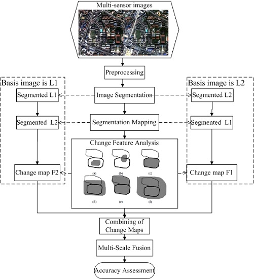
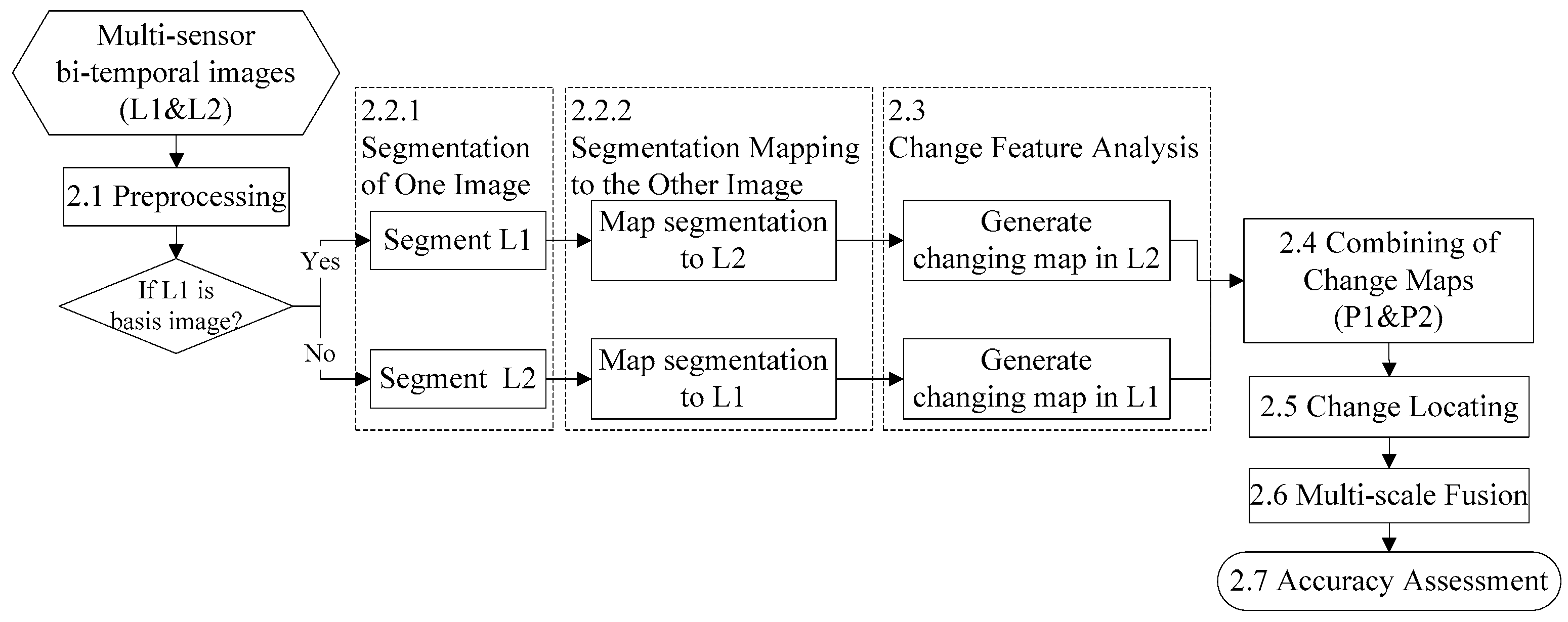
The processing flow of the proposed method is shown in Figure 1.
2.1. Preprocessing
In the preprocessing of the proposed method, image resampling is conducted to unify the size of the multi-sensor bi-temporal images. The bilinear resampling method is adopted to suppress the image heterogeneity, with a reasonable computation cost [38]. When the basis image is the one with a higher spatial resolution, the other image needs to be interpolated by up-sampling. Otherwise, the image is degraded by down-sampling to the lower resolution of the basis image.
2.2. Image Segmentation
Image segmentation is implemented to obtain image objects for the subsequent object-based processes. In this paper, there are three objectives for the image segmentation: (1) the bi-temporal image objects should be in one-to-one correspondence; (2) the spatial distribution between changed objects and their relevant changed areas needs to be preserved for the subsequent change feature analysis (Section 2.3); and (3) the objects obtained from slight under-segmentation are better able to fit the edges of the changed areas in the other image. Therefore, we propose to segment one of the bi-temporal images and map the segmentation to the other. These two segmentation processes are introduced below.
2.2.1. Segmentation of One Image
The segmentation of one image should take into account the spectral and spatial features of the ground objects. In addition, as mentioned above, the image objects should be slightly under-segmented to fit the edges of the changed areas in the other image. In this paper, we use the fractal net evolution approach (FNEA) [39] for the image segmentation. This approach involves calculating the heterogeneity () between each pair of neighboring objects according to Equation (1), which is a weighted sum of the spectral and spatial criteria:
where is the user-defined weight of the spectral feature. The sum of the weights of the spectral and spatial criteria equals 1. If the spectral feature is emphasized in the segmentation, the value of should be larger. Conversely, the value of , which is the weight of the spatial feature, should be larger when the spatial feature is more important. and are, respectively, the spectral and spatial heterogeneity, whose definition can be found in [39].
At the beginning of the segmentation, every pixel is regarded as an individual object. After calculating the heterogeneity () of each pair of neighboring objects, they are compared to the value of the scale, which can be regarded as the threshold of the heterogeneity:
- (1)
- If < scale, this pair of objects are merged;
- (2)
- Otherwise, the objects are preserved as two individual objects.
This procedure is repeated until no objects can be merged, and the object map is obtained. The scale is critical to the segmentation as it determines the size of the objects.
Using FNEA, only the scale parameter needs to be selected to adjust the size of the image objects. We can make use of Definiens software (Definiens, München, Germany) to simply implement this method. On the premise of efficiency, other segmentation methods [40,41] could also be adopted in the proposed method.
2.2.2. Segmentation Mapping to the Other Image
In this paper, we simply map the segmentation of one image to the other. In this way, the bi-temporal image objects are in one-to-one correspondence. In addition, the spatial distribution between changed objects and their relevant changed areas are also preserved, which is critical for the following change feature analysis.
2.3. Change Feature Analysis
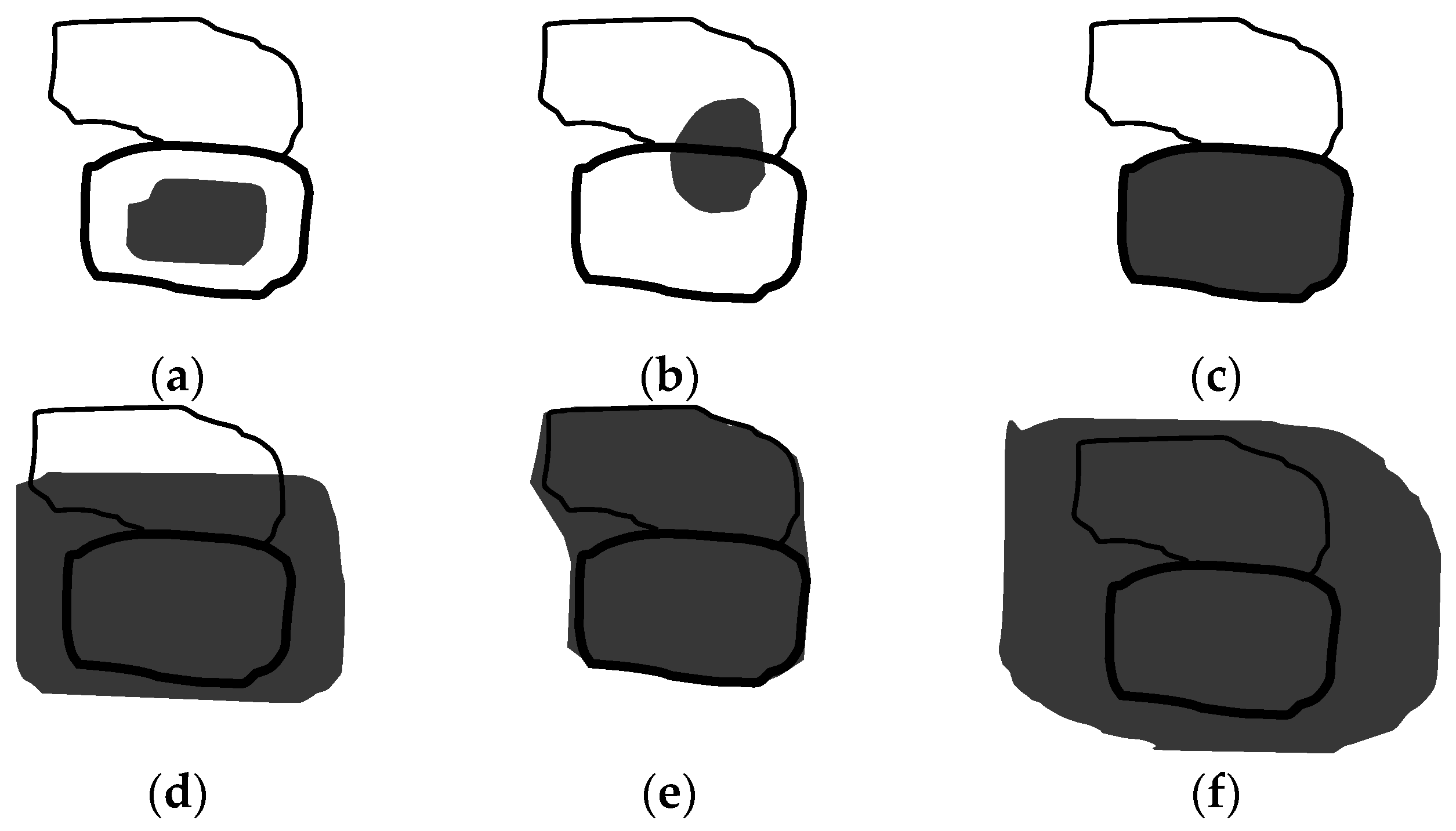
After mapping the segmentation of one image to the other, there will be different spatial distributions between a changed object and its relevant changed area. Figure 2 shows the possible distributions of a changed object and its relevant changed area, in which the bold object represents a changed object, and the object above it is one of its neighboring objects. The shadow area represents the relevant changed area. Through analyzing the six possible distributions in Figure 2, we can deduce the statistical feature variation of the changed objects as follows:
Denoting the bi-temporal images as L1 and L2 and mapping the segmentation of L1 to L2,
- (a)
- if the relevant changed area is contained in the changed object, the standard deviation of the changed object in L2 is larger than L1 (Figure 2a);
- (b)
- if the relevant changed area covers parts of the changed object and its neighborhood, the contrast between the changed object and its neighboring pixels in L2 is less than L1 (Figure 2b);
- (c)
- if the relevant changed area exactly covers the changed object, the ratio of contrast between the changed object and its neighboring pixels in L1 and L2 is not equal to 1 (Figure 2c);
- (d)
- if the relevant changed area covers the whole changed object and parts of its neighborhood, the contrast between the changed object and its neighboring pixels in L2 is less than L1 (Figure 2d);
- (e)
- if the relevant changed area exactly covers the changed object and its neighboring object, the contrast between the changed object and its neighboring pixels in L2 is less than L1 (Figure 2e); and
- (f)
- if the relevant changed area exceeds the changed object and its neighboring object, the contrast between the changed object and its neighboring pixels in L2 is less than L1 (Figure 2f).
According to the above statistical feature variations of changed objects, we define a change feature (Equations (2) and (3)) to describe the statistical features of the image objects in bi-temporal MS images. The change feature adequately takes into account the statistical features of the image objects in the bi-temporal images (acquired by the same or different satellites), which is an important innovation of the proposed method.
If :
otherwise:
where is the change feature value for object i, and is the ratio of contrast between object i and its neighboring pixels in L1 and L2. is the contrast between object i and its neighboring pixel (i, j), and is the standard deviation of object i. is the set of pixels adjacent to object i.
The ratio of contrast between the changed object and its neighboring pixels in L1 and L2 can be defined as:
where and represent the contrast between object i and its neighboring pixel (i, j) in L1 and L2, respectively.
The contrast between the changed object and one of its neighboring pixels can be defined as:
where is the mean value of the pixels in object i, and is the value of the neighboring pixel (i, j).
The standard deviation of the changed object is defined as:
where ni is the number of neighboring pixels in object i, and Obji is the set of pixels in object i.
According to the proposed change feature of image objects, there are three statistical factors related to the changes:
- (1)
- the ratio of contrast between any object and its neighboring pixels in L1 and L2;
- (2)
- the sum of contrast between any object and each of its neighboring pixels; and
- (3)
- the standard deviation value of any object.
In other words, if any image object is related to local changes, one of these three factors would vary between the bi-temporal images, and the proposed change feature of this object in L2 would be less in L1. Consequently, the change map in L2 can be generated by representing each object with the change probability:
2.4. Combining the Change Maps
In order to preserve the change information as much as possible, the bi-temporal images take turns to be segmented and mapped to each other. The pair of change maps is combined as:
where is the combined change probability of object i. and represent the change probabilities of object i by respectively segmenting L1 and L2 and mapping them to each other. and are the weights of the change maps. Subsequently, the combined change map can be used for locating the changes. The combination ratio of change maps is an important parameter in this method, which is confirmed in the experiments (Section 3).
2.5. Change Locating
The changes are located by discriminating them from unchanged areas in the combined change map. Since the combined change map represents the change probability of each gray-level image object, the change locating can be realized by setting a threshold to divide the map into two parts, or applying a binary unsupervised classification method. In this paper, two threshold selection techniques, Otsu’s thresholding method [42] and “threshold selection by clustering gray levels of boundary” [43], and k-means clustering [44] (k = 2) are used to extract the changes in the combined change map. These methods could also be replaced by other thresholding or clustering methods [45,46,47], in which [45] effectively improved the band selection of hyperspectral imagery concerning on dual clustering. However, it is confirmed to have little effect on the proposed method (see Section 3).
(1) Otsu’s thresholding method
Otsu’s thresholding method is implemented by searching for the optimal threshold to maximize the discrimination criterion and achieve the greatest separability of classes. The criterion is defined as:
where C is the criterion value of an image unit (pixel or object), and is the mean of the gray levels in the image. and are the zeroth- and first-order cumulative moments of the histogram up to the k-th gray level, respectively. The optimal threshold is obtained by maximizing the value of C. In this paper, Otsu’s thresholding method is used to find the optimal threshold to separate the changes and unchanged areas in the combined change map.
(2) Threshold selection by clustering gray levels of boundary
The threshold selection by clustering gray levels of boundary method involves approximating the mean of the discrete sample pixels lying on the boundary and separating the image into objects and background. The image is divided into square grids, and classified into edge cells intersected by boundary and non-edge cells. Mathematically, the boundary of the image can be represented as:
where and are the Laplacian and gradient magnitude functions of pixel (x, y), respectively. If any edge of an edge cell is intersected by the boundary, the edge has the following properties:
- (a)
- its two vertices (p1 and p2) are a pair of zero-crossing points, namely, ; and
- (b)
- its two vertices (p1 and p2) both have high gradient values. For a predefined gradient threshold , .
In this way, the intersected pixels of edge cells on the boundary can be obtained. Their positions and gray values are computed by linear interpolation of the two vertices on the edge. These intersected pixels are regarded as the discrete sample pixels on the image boundary. The mean of their gray values is used as the threshold for the image segmentation. In this study, in order to divide the combined change map into changed and unchanged classes, this threshold selection method is used to find a bi-level threshold in the feature map.
(3) K-means clustering
K-means clustering is a classical unsupervised classification method. It involves clustering image pixels according to the similarity of their gray levels. The number of clusters depends on the specific application and is defined by the user. In this paper, k-means clustering (k = 2) is used to classify the combined change map—a gray-level image—into two classes of changed and unchanged areas.
2.6. Multi-Scale Fusion
Considering the multi-scale characteristic of ground objects, multi-scale fusion [30] is applied in the proposed method. The multi-scale fusion is implemented by voting from the single-scale change detection maps. Firstly, we choose an appropriate interval for the segmentation scale, which needs to cover most of the image objects’ sizes. We repeat the processes of the proposed method from steps 2.1 to 2.5 (in Figure 1) by increasing the scale with a constant step size, and we obtain a set of single-scale change detection maps. The image objects in these maps only have two values—0 and 1—which, respectively, mean unchanged and changed objects. The sum of the single-scale change detection maps is calculated as:
where Sji is the value of object i in single-scale change detection map j. Mi is the sum of object i in all of the single-scale change detection maps, and n is the number of single-scale change detection maps. The multi-scale change detection map is defined as:
where Fi is the value of image object i in the multi-scale change detection map, in which 0 and 1, respectively, mean unchanged and changed objects. Tf is the threshold of the multi-scale fusion.
In this way, if an image object is changed in more than Tf single-scale change detection maps, it is recognized as changed after the multi-scale fusion. Especially, the changed areas after the multi-scale fusion are the sum and the intersection of the changes in all the single-scale change detection maps, when Tf is equal to 0 and 1, respectively.
In the experiments described in Section 3, the optimal result of the multi-scale fusion is the sum of changes in all the single-scale change detection maps, in which Tf is equal to 0.
2.7. Accuracy Assessment
In this paper, false alarms, missed alarms, and overall errors are used to assess the accuracy of the urban change detection. False alarms mean the ratio of unchanged pixels wrongly detected as changed, and missed alarms are the ratio of changed pixels omitted in the change detection. Consequently, overall errors, which is the integrated ratio of the wrongly detected and omitted changed pixels in the image, estimates the effectiveness of the change detection method [30].
Furthermore, in order to validate the effectiveness of the proposed method, it was compared with some of the existing methods. The most important innovations of the proposed method are that it takes into account the incompatibility between different bandwidths and uses an object-based change measure in the multi-sensor MS images. Since there are no other object-based change detection methods for multi-sensor images, we chose to compare the proposed method with the method proposed in [35], which utilizes some features that are invariant to change in the illumination conditions to undertake change detection in multi-sensor images.
3. Experiments
3.1. The First Study Area
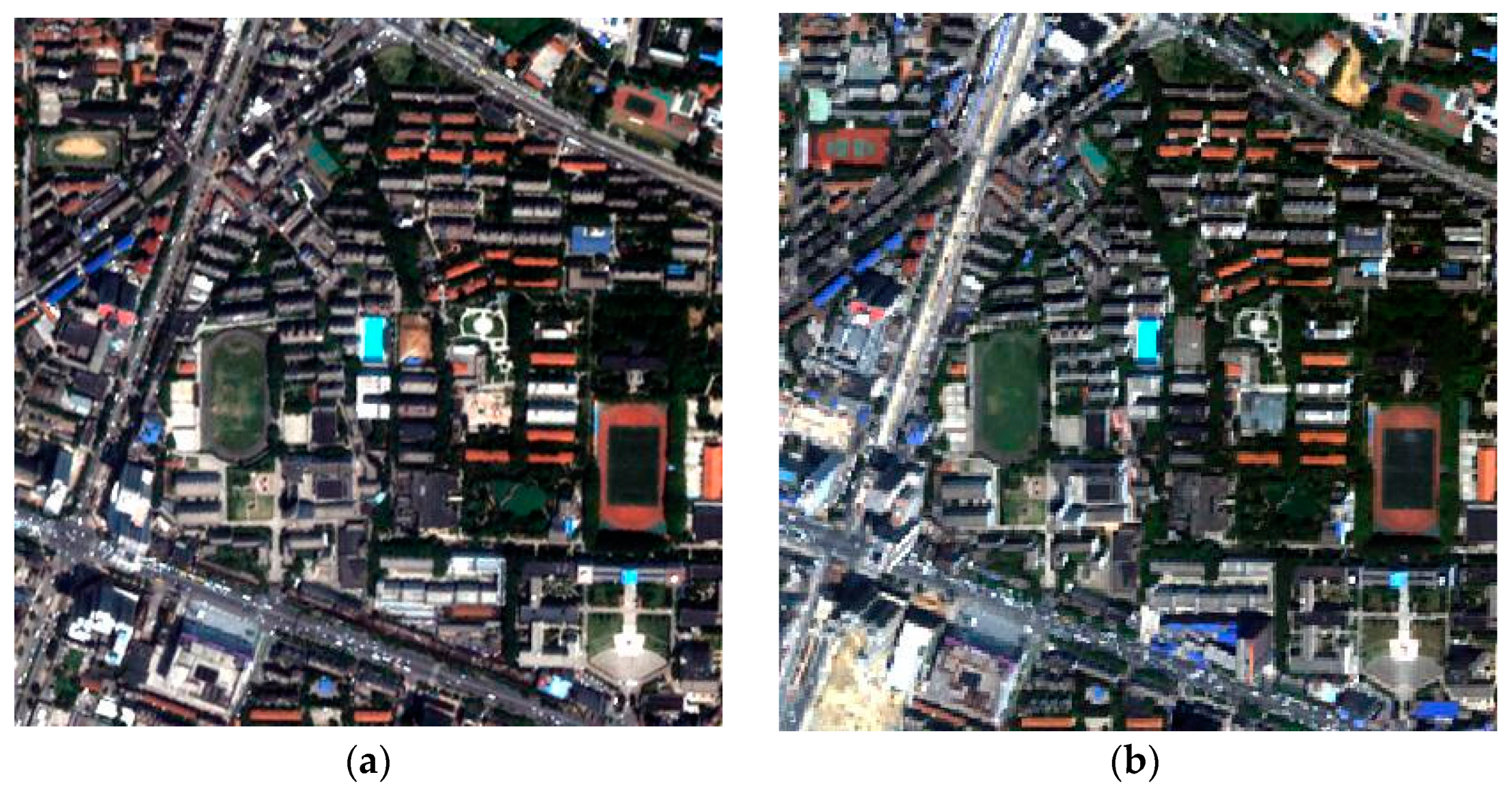
The first study area covers the campus of Wuhan University in Hubei province of China. The bi-temporal images were respectively acquired by the QuickBird satellite in April 2005 (L1) and the IKONOS satellite in July 2009 (L2). In order to preserve the spectral information, the MS images were used in the experiments. Although there were four bands in both images, their spectral and spatial characteristics differed as they were acquired by different sensors (Table 1). Either L1 or L2 can be viewed as the basis image in the image resampling preprocessing.
1. L1 as the basis image
With L1 as the basis image, L2 was interpolated to the spatial resolution of L1. Figure 3 shows the bi-temporal images after the interpolation, which are both 400 × 400 pixels. In order to avoid the effects of vegetation phenology and solar elevation, the vegetation and shadow were extracted and masked out.
By mapping the segmentation of L1 to L2, a change map was generated by calculating the value of the change probability (Equation (7)) for each object. The other change map was obtained by exchanging the order of the two images. With different ratios for combining these maps, the characteristics of the combined changed maps varied.
In order to determine the change locations, it is crucial to discriminate the changes from the unchanged areas in the combined change map. The two threshold selection techniques and k-means clustering (k = 2) (introduced in Section 2.5) were used to analyze the combined change map. The results of the three methods are shown in Table 2. In this table, the left, middle, and right parts, respectively, show false, missed alarms, and overall errors among the three methods with different combining ratios of change maps. It can be seen that the overall errors of the three methods are similar. The k-means clustering (k = 2) obtains the smallest number of errors, and the threshold selection by clustering gray levels of boundary method performs a little better than Otsu’s thresholding method. Moreover, with the increase of the combination ratio of the change maps, the overall errors of each method decrease. This is because, in Equation (8), P2 and P1 represent the change probability of L2 and L1, which was mapped from the segmentation of L1 and L2, respectively. As L2 was interpolated to the spatial resolution of L1, the segmentation of L1 was more accurate than the segmentation of L2. Therefore, a larger weight of P2 leads to a higher accuracy of change feature analysis.
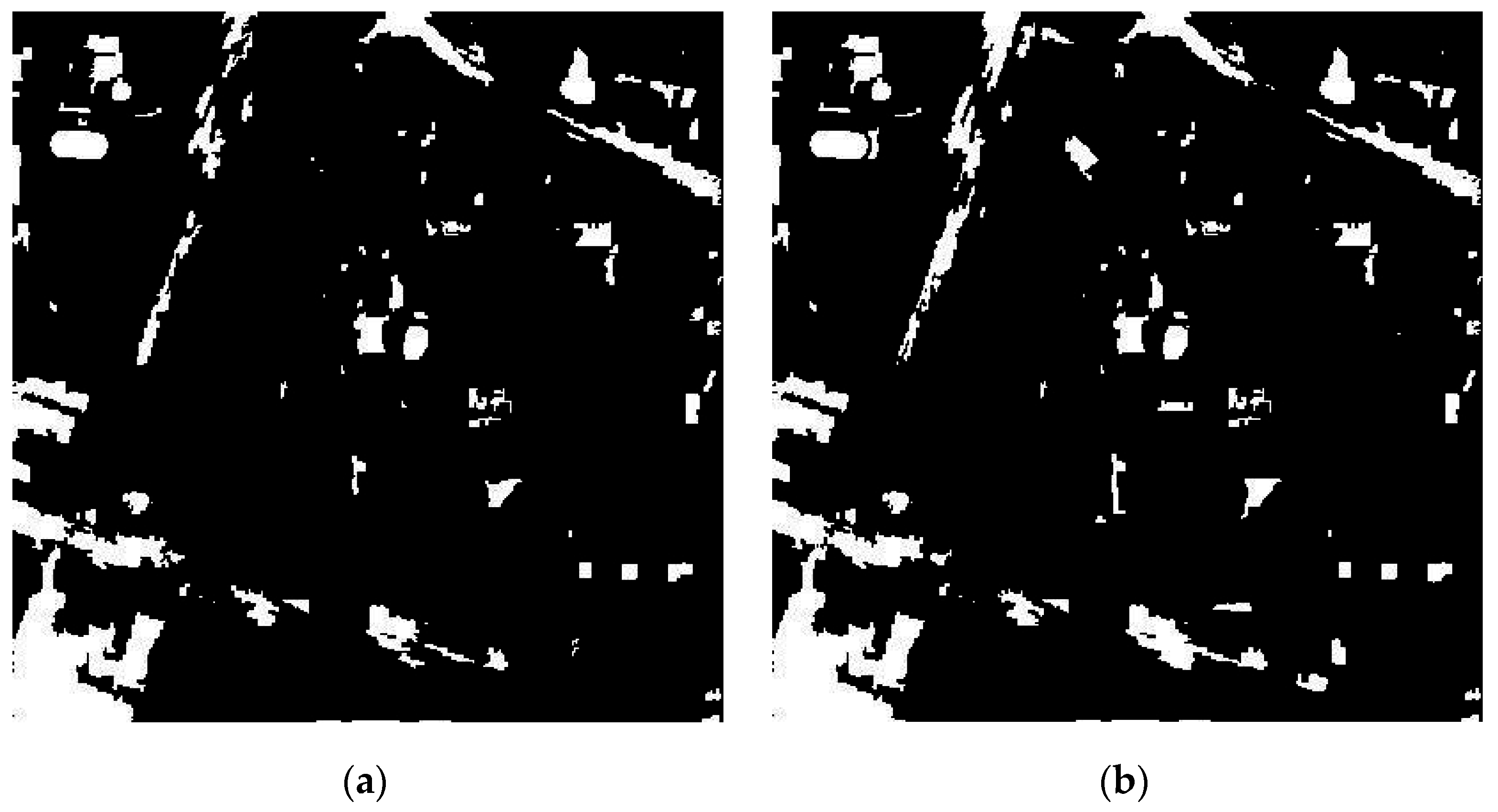
The results are visually compared in Figure 4, in which the white and black regions, respectively, represent the changed and unchanged areas. The results of the three methods are similar, but the number of false alarms for k-means clustering (k = 2) is slightly more than for the other two methods, and the missed alarms are fewer in number, especially in the road areas.
According to the spatial resolution and the objects’ sizes in the bi-temporal images after preprocessing, the scale interval and step size increase were set as [10, 150] and 10, respectively. The results of the change feature analysis differ with the varying segmentation scales (Figure 5), and the optimal scale is around 100. Considering the multi-resolution characteristics of ground objects, multi-scale fusion is applied in the proposed method, and is realized by voting from the single-scale binary change maps. Figure 6 shows the accuracy of the k-means clustering (k = 2) after the multi-scale fusion. The overall errors are the lowest when Tf in Equation (13) is 0, which means that the optimal multi-scale fusion is the sum of the changes in all of the single-scale change detection maps.
The accuracies of both the single-scale and multi-scale proposed method are shown in Table 3. As the multi-scale fusion integrates all the single-scale change maps, there are more false alarms but fewer missed alarms than for the optimal single-scale method. Comparing the overall errors, the multi-scale version is more accurate.
Moreover, in order to validate the effectiveness of the proposed change detection method for multi-sensor MS imagery, it was compared with the method proposed in [35]. In Figure 7, the white and black regions represent the changed and unchanged areas, respectively. It can be seen that the proposed method effectively decreases the false alarms and suppresses the salt-and-pepper noise in the changed areas. As there are great differences in the visual results, the quantitative assessment and comparison are omitted. The time costs of the two methods were both less than two minutes using MATLAB Software (Mathworks, Natick, MA, USA) on a personal computer with 1.80 GHz CPU and 8.00 GB RAM.
2. L2 as the basis image
In this experiment, L2 was used as the basis image in the preprocessing. Having a higher spatial resolution, L1 was degraded to the same resolution as L2. Figure 8 shows the bi-temporal images after the down-sampling, which are both 240 × 240 pixels. The vegetation and shadow were again masked out.
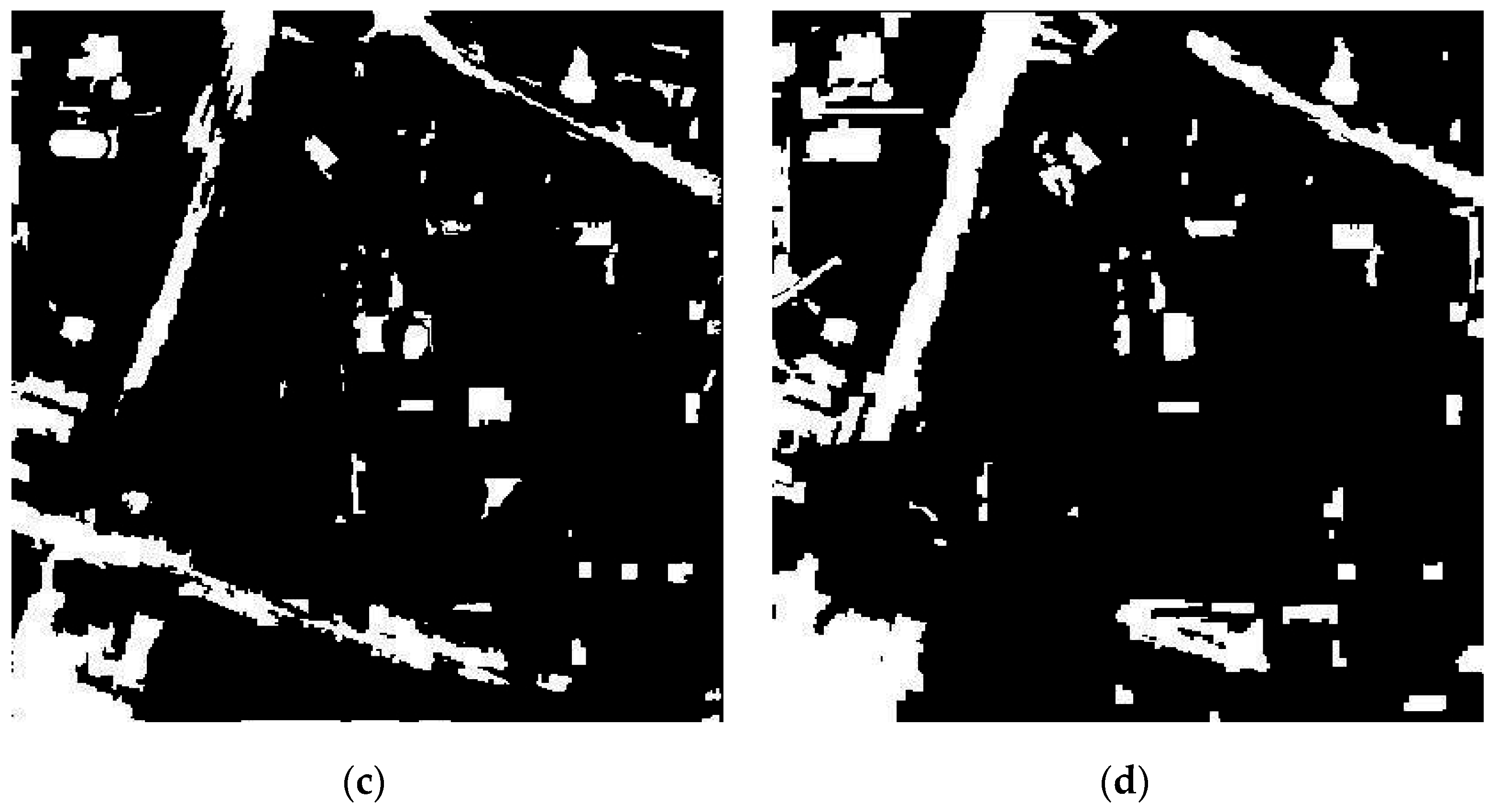
In the analysis of the combined change map, the two threshold selection methods and k-means clustering (k = 2) were again used. The results are shown in Table 4. In this table, the left, middle, and right parts, respectively, show false, missed alarms, and overall errors among the three methods with increasing ratio of P2. It can be seen that the overall errors of the three methods are again similar. The k-means clustering (k = 2) obtains the least number of errors, and the threshold selection by clustering gray levels of boundary method performs slightly better than Otsu’s thresholding method. Figure 9 shows a visual comparison of the results, in which the white and black regions represent the changed and unchanged areas, respectively. The results of the three methods are again similar, and the k-means clustering (k = 2) obtains slightly fewer missed alarms than the two threshold selection methods, which is the same as the result of the experiment with L1 as the basis image.
However, it is worth noting that the overall errors increase with the decreasing combination ratio of P1. This is probably because the down-sampling of L1 resulted in the loss of some valuable image information. As a result, the change map of P1, which was generated by the change feature analysis of L1 mapped from the segmentation of L2, was more accurate than the other change map. Therefore, a larger weight of P1 in the combined change map leads to a higher accuracy. From the results of these experiments, we can conclude that the accuracy of the change analysis is improved by increasing the weight of the change map which is generated by mapping the segmentation of the basis image.
According to the spatial resolution and the objects’ sizes in the bi-temporal images after preprocessing, the scale interval and step size increase were set as [10, 100] and 10, respectively. Figure 10 shows the results of the proposed single-scale method using different segmentation scales. The optimal scale is 50. As can be seen in Figure 6, the overall errors are the lowest when Tf in Equation (13) is 0. In addition, Table 5 shows the improvement of the multi-scale fusion with Tf equal to 0, which was realized by k-means clustering (k = 2).
In Figure 11, the proposed method is compared with the method proposed in [35]. The white and black regions represent the changed and unchanged areas, respectively. It can be seen that the proposed method is better able to detect the changes in an urban area with multi-sensor MS images. It suppresses the missed alarms in the changed areas and decreases the false alarms. As there is a significant difference in the visual results, the quantitative assessment and comparison are omitted. The time costs of the two methods were both about one minute using MATLAB Software (Mathworks, Natick, MA, USA) on a personal computer with 1.80 GHz CPU and 8.00 GB RAM.
Comparing the two sets of experiments in the first study area, the accuracy is higher in the results with L2 as the basis image. This is probably due to the lower spatial resolution of the basis image.
3.2. The Second Study Area
In order to further verify the proposed method, it was also applied to images from another area in the south of Wuhan, Hubei province, China. The bi-temporal images were respectively acquired by QuickBird in April 2002 (L1) and by IKONOS in July 2009 (L2). L2, with the lower resolution, was regarded as the basis image in the preprocessing, and L1 was degraded by down-sampling. The images after reprocessing, with a size of 240 × 240 pixels, are shown in Figure 12. The vegetation and shadow were, again, masked out to avoid the effects of vegetation phenology and solar elevation.
As the spatial resolutions were the same and the ground objects of the urban area were similar to those of the first study area, the segmentation scale was again set to 50. The results of the two threshold selection methods and k-means clustering (k = 2) are compared in Table 6, with a decreasing P1 ratio. In this table, the left, middle, and right parts, respectively, show false, missed alarms, and overall errors among the three methods with decreasing ratio of P1. The accuracies of the three change locating methods are again similar. K-means clustering (k = 2) performs the best, and the threshold selection by clustering gray levels of boundary method performs slightly better than Otsu’s thresholding method, which is the same as the first study area. As with the results in the first study area, the accuracy of the proposed method is improved by increasing the weight of P1, which is generated by mapping the segmentation of the basis image of L2. Therefore, it can be concluded that if the weight of the change map, which is mapped from the segmentation of the basis image, is larger than the other, the accuracy of the proposed method increases.
The binary change maps of the three methods are shown in Figure 13, in which the white and black regions represent the changed and unchanged areas, respectively. Compared with the reference image, the results of the three methods are similar, and the k-means clustering (k = 2) obtains the least number of missed alarms.
As can be seen in Figure 6, the overall errors after the multi-scale fusion are the lowest when Tf in Equation (13) is 0. Table 7 shows the improvement of the multi-scale fusion with Tf equal to 0, which was realized by k-means clustering (k = 2). It can be concluded that the proposed multi-scale method suppresses the missed alarms and keeps the false alarms to an acceptable level.
In Figure 14, the white and black regions represent the changed and unchanged areas, respectively. Compared with the method proposed in [35], the proposed method is shown to be effective in detecting changes in an urban area using multi-sensor MS images. It can effectively decrease the missed alarms in the changed areas while removing the false alarms. As there is a great difference in the visual results, the quantitative assessment and comparison are omitted. The time costs of the two methods were both about one minute using MATLAB Software (Mathworks, Natick, MA, USA) on a personal computer with 1.80 GHz CPU and 8.00 GB RAM.
4. Discussion
In this paper, we have described the experiments conducted with multi-sensor MS images acquired by QuickBird and IKONOS in two different study areas. According to the results of the experiments, the following conclusions can be made:
(1) In the preprocessing of the proposed method, using the image with a lower resolution as the basis image can improve the change detection accuracy. This is probably because some redundant information is removed in the image with lower resolution.
(2) We made use of commercial software (Definiens) to carry out the FNEA and adjust the scale of the image objects to achieve slight under-segmentation. FNEA could be replaced by other segmentation methods, whose results are similar to FNEA.
(3) A change feature is defined to estimate the change possibility of image objects in bi-temporal MS images. The change feature adequately takes into account the statistical features of the image objects in the bi-temporal images (whether acquired by the same or different satellites), which is an important innovation of the proposed method.
(4) In the combining of the change maps, greater precision can be achieved by increasing the ratio of the map which is generated from mapping the segmentation of the basis image to the resampled one. This is probably because the segmentation of the basis image is more precise than the resampled one.
(5) The results of both thresholding and clustering methods for the change locating in gray-level images of the change probability are similar, which confirms that they have little effect on the proposed method.
(6) The multi-scale fusion can effectively improve the accuracy by suppressing the missed alarms and keeping the false alarms to an acceptable level. The overall errors after the multi-scale fusion are the lowest when the changed areas are the sum of the changes in all the single-scale change detection maps.
(7) Compared with the method proposed in [35], the proposed method can effectively detect the changes in multi-sensor MS images by suppressing the missed and false alarms. Instead of utilizing features invariant to different the illumination conditions, the proposed method takes into account the incompatibility between different bandwidths and uses an object-based change measure with the multi-sensor MS images.
5. Conclusions
In this paper, a novel object-based change detection method has been proposed for multi-sensor MS imagery. After the resampling preprocessing, we segment one of the bi-temporal images and map it to the other image, which not only achieves one-to-one correspondence between the bi-temporal images but also preserves the spatial distribution between changed objects and their relevant changed areas. Subsequently, by summarizing the possible distribution between any image object and its relevant changed areas, a change feature is defined to represent the change probability of the image objects in the bi-temporal MS images, whether they are acquired by the same or different satellites. Consequently, thresholding or clustering methods are used to automatically locate the changes in the gray-level image of change probability. Considering the multi-scale feature of ground objects, multi-scale fusion is implemented by voting from the single-scale maps.
According to the experimental results, the urban change analysis method proposed in this paper effectively overcomes the incompatibility between different band widths in bi-temporal (MS) images and utilizes object-based statistical features to describe the changes of ground objects. The overall errors of the proposed method are less than 3.5%. The proposed method makes full use of the spectral and spatial information, and it estimates the change probability of image objects by the use of a novel statistical feature. The object-based change detection method can effectively detect the changes in multi-sensor MS images, and has been confirmed to perform better than the current methods.
Acknowledgments
The authors appreciate the guidance of Prof. Xin Huang from Wuhan University of China. This work was supported by the National 973 Plan of China (grant no. 2012CB719903), the National Natural Science Foundation of China (grant nos. 41401402, 41301453, and 51479215), the Natural Science Foundation of Hunan Province in China (grant no. 2015JJ3150), the Geographical Conditions Monitoring Project of Hunan Province in China (grant no. HNGQJC201503), the Open Research Fund Program of the Key Laboratory of Earth Observation, the State Bureau of Surveying and Mapping (grant no. K201504), the Major Project of High Resolution Earth Observation System of China (Civil Part) (grant no. 03-Y20A11-9001-15/16), and the Demonstration System of High-Resolution Remote Sensing Application in Surveying and Mapping of China (grant no. AH1601-8).
Author Contributions
Yuqi Tang designed the proposed mode, implemented the experiments and drafted the manuscript. Liangpei Zhang provided overall guidance to the project, reviewed and edited the manuscript.
Conflicts of Interest
The authors declare no conflict of interest.
References
- Ingram, K.; Knapp, E.; Robinson, J.W. Change Detection Technique Development for Improved Urbanized Area Delineation. In Technical Memorandum, CSC/TM-81/6087; Computer Sciences Corporation: Silver Springs, MD, USA, 2004. [Google Scholar]
- Bruzzone, L.; Bovolo, F. A novel framework for the design of change-detection systems for very-high-resolution remote sensing images. Proc. IEEE 2013, 101, 609–630. [Google Scholar] [CrossRef]
- Tang, Y.; Huang, X.; Zhang, L. Fault-tolerant building change detection from urban high-resolution remote sensing Imagery. IEEE Geosci. Remote Sens. Lett. 2013, 10, 1060–1064. [Google Scholar] [CrossRef]
- Bruzzone, L.; Fernandez-Prieto, D. Automatic analysis of the difference image for unsupervised change detection. IEEE Geosci. Remote Sens. Lett. 2000, 38, 1170–1182. [Google Scholar] [CrossRef]
- Celik, T.; Ma, K.K. Unsupervised change detection for satellite images using dual-tree complex wavelet transform. IEEE Geosci. Remote Sens. Lett. 2012, 48, 1199–1210. [Google Scholar] [CrossRef]
- Bazi, Y.; Melgani, F.; Al-Sharari, H.D. Unsupervised change detection in multispectral remotely sensed imagery with level set methods. IEEE Geosci. Remote Sens. Lett. 2010, 48, 3178–3187. [Google Scholar] [CrossRef]
- Bovolo, F.; Bruzzone, L. A theoretical framework for unsupervised change detection based on change vector analysis in polar domain. IEEE Geosci. Remote Sens. Lett. 2007, 45, 218–236. [Google Scholar] [CrossRef]
- Bovolo, F.; Marchesi, S.; Bruzzone, L. A framework for automatic and unsupervised detection of multiple changes in multitemporal images. IEEE Geosci. Remote Sens. Lett. 2012, 50, 2196–2212. [Google Scholar] [CrossRef]
- Celik, T. Change detection in satellite images using a genetic algorithm approach. IEEE Geosci. Remote Sens. Lett. 2010, 7, 386–390. [Google Scholar] [CrossRef]
- Heng, C.; Celik, T.; Longbotham, N.; Emery, W.J. Gabor feature based unsupervised change detection of multitemporal SAR images based on two-level clustering. IEEE Geosci. Remote Sens. Lett. 2015, 12, 2458–2462. [Google Scholar] [CrossRef]
- Nielsen, A.A. Multiset canonical correlations analysis and multispectral, truly multitemporal remote sensing data. IEEE Trans. Image Process. 2002, 11, 293–305. [Google Scholar] [CrossRef] [PubMed] [Green Version]
- Marchesi, S.; Bovolo, F.; Bruzzone, L. A context-sensitive technique robust to registration noise for change detection in VHR multispectral images. IEEE Trans. Image Process. 2010, 19, 1877–1889. [Google Scholar] [CrossRef] [PubMed]
- Nielsen, A.A.; Conradsem, K.; Simpson, J.J. Multivariate alteration detection(MAD) and MAF postprocessing in multispectral bitemporal image data: New approaches to change detection studies. Remote Sens. Environ. 1998, 64, 1–19. [Google Scholar] [CrossRef]
- Marpu, P.R.; Gamba, P.; Canty, M.J. Improving change detection results of IR-MAD by eliminating strong changes. IEEE Geosci. Remote Sens. Lett. 2011, 8, 799–803. [Google Scholar] [CrossRef]
- Nielsen, A.A. The regularized iteratively reweighted MAD method for change detection in multi- and hyperspectral data. IEEE Geosci. Remote Sens. Lett. 2007, 16, 463–478. [Google Scholar] [CrossRef]
- Wang, Q.; Lin, J.; Yuan, Y. Salient band selection for hyperspectral image classification via manifold ranking. IEEE Trans. Neural Netw. Learn. Syst. 2016, 27, 1279–1289. [Google Scholar] [CrossRef] [PubMed]
- Yuan, Y.; Zhu, G.; Wang, Q. Hyperspectral band selection by multi-task sparsity pursuit. IEEE Geosci. Remote Sens. Lett. 2015, 53, 631–644. [Google Scholar] [CrossRef]
- Luo, W.; Li, H. Soft-change detection in optical satellite images. IEEE Geosci. Remote Sens. Lett. 2011, 8, 879–883. [Google Scholar] [CrossRef]
- Ling, F.; Li, W.; Du, Y.; Li, X. Land cover change mapping at the subpixel scale with different spatial-resolution remotely sensed imagery. IEEE Geosci. Remote Sens. Lett. 2011, 8, 182–186. [Google Scholar] [CrossRef]
- Robin, A.; Moisan, L.; Hegarat-Mascle, S.L. An a-contrario approach for subpixel change detection in satellite imagery. IEEE Trans. Pattern Anal. Mach. Intell. 2010, 32, 1977–1993. [Google Scholar] [CrossRef] [PubMed] [Green Version]
- Gueguen, L.; Soille, P.; Pesaresi, M. Change detection based on information measure. IEEE Geosci. Remote Sens. Lett. 2011, 49, 4503–4515. [Google Scholar] [CrossRef]
- Healey, G.; Slater, D. Computing illumination-invariant descriptors of spatially filtered color image regions. IEEE Trans. Image Process. 1997, 6, 1002–1013. [Google Scholar] [CrossRef] [PubMed]
- Smits, P.C.; Annoni, A. Updating land-cover maps by using texture information from very high-resolution space-borne imagery. IEEE Geosci. Remote Sens. Lett. 1999, 37, 1244–1254. [Google Scholar] [CrossRef]
- Li, L.; Leung, M.K.H. Integrating intensity and texture differences for robust change detection. IEEE Trans. Image Process. 2002, 11, 105–112. [Google Scholar] [PubMed]
- Moser, G.; Angiati, E.; Serpico, S.B. Multiscale unsupervised change detection on optical images by Markov random fields and wavelets. IEEE Geosci. Remote Sens. Lett. 2011, 8, 725–729. [Google Scholar] [CrossRef]
- Yuan, Y.; Lin, J.; Wang, Q. Hyperspectral image classification via multi-task joint sparse representation and stepwise MRF optimization. IEEE Trans. Cybern. 2016, 46, 2966–2977. [Google Scholar] [CrossRef] [PubMed]
- Dalla Mura, M.; Benediktsson, J.A.; Bovolo, F.; Bruzzone, L. An unsupervised technique based on morphological filters for change detection in very high resolution images. IEEE Geosci. Remote Sens. Lett. 2008, 5, 433–437. [Google Scholar] [CrossRef]
- Dalla Mura, M.; Benediktsson, J.A.; Waske, B.; Bruzzone, L. Morphological attribute profiles for the analysis of very high resolution images. IEEE Geosci. Remote Sens. Lett. 2010, 48, 3747–3762. [Google Scholar] [CrossRef]
- Im, J.; Jensen, J.R.; Tullis, J.A. Object-based change detection using correlation image analysis and image segmentation. Int. J. Remote Sens. 2008, 29, 399–423. [Google Scholar] [CrossRef]
- Bovolo, F. A multilevel parcel-based approach to change detection in very high resolution multitemporal images. IEEE Geosci. Remote Sens. Lett. 2009, 6, 33–37. [Google Scholar] [CrossRef]
- Lu, P.; Stumpf, A.; Kerle, N.; Casagli, N. Object-oriented change detection for landslide rapid mapping. IEEE Geosci. Remote Sens. Lett. 2011, 8, 701–705. [Google Scholar] [CrossRef]
- Huo, C.; Zhou, Z.; Lu, H.; Pan, C.; Chen, K. Fast object-level change detection for VHR images. IEEE Geosci. Remote Sens. Lett. 2010, 7, 118–122. [Google Scholar] [CrossRef]
- Tang, Y.; Zhang, L.; Huang, X. Object-oriented change detection based on the Kolmogorov-Smirnov test using high-resolution multispectral imagery. Int. J. Remote Sens. 2011, 32, 5719–5740. [Google Scholar] [CrossRef]
- Mercier, G.; Moser, G.; Serpico, S. Conditional copulas for change detection in heterogeneous remote sensing images. IEEE Trans. Geosci. Remote Sens. 2008, 46, 1428–1441. [Google Scholar] [CrossRef]
- Habib, A.; AI-Ruzouq, R.; Kim, C. Semi-automatic registration and change detection using multi-source imagery with varying geometric and radiometric properties. Int. Arch. Photogramm. Remote Sens. Spat. Inf. Sci. 2012, 1, 1–6. [Google Scholar]
- Bovolo, F.; Bruzzone, L.; Marconcini, M. A novel approach to unsupervised change detection based on a semisupervised SVM and a similarity measure. IEEE Trans. Geosci. Remote Sens. 2008, 46, 2070–2082. [Google Scholar] [CrossRef]
- Thonfeld, F.; Feihauer, H.; Braun, M.; Menz, G. Robust change vector analysis (RVCA) for multi-sensor very high resolution optical satellite data. Int. J. Appl. Earth Obs. Geoinform. 2016, 51, 131–140. [Google Scholar] [CrossRef]
- Richards, J. Remote Sensing Digital Image Analysis: An Introduction; Springer: Berlin/Heidelberg, Germany, 1986; pp. 52–55. [Google Scholar]
- Baatz, M.; Schape, A. Multiresolution Segmentation: An Optimization Approach for High Quality Multi-Scale Image Segmentation; Wichmann-Verlag: Heidelberg, Germany, 2000; pp. 12–23. [Google Scholar]
- Pesaresi, M.; Benediktsson, J.A. A new approach for the morphological segmentation of high-resolution satellite imagery. IEEE Trans. Geosci. Remote Sens. 2011, 39, 309–320. [Google Scholar] [CrossRef]
- Huang, X.; Zhang, L. An adaptive mean-shift analysis approach for object extraction and classification from urban hyperspectral imagery. IEEE Trans. Geosci. Remote Sens. 2008, 46, 4173–4185. [Google Scholar] [CrossRef]
- Otsu, N. A threshold selection method from gray-level histograms. IEEE Trans. Syst. Man Cybern. 1979, 9, 61–66. [Google Scholar] [CrossRef]
- Wang, L.; Bai, J. Threshold selection by clustering gray levels of boundary. Pattern Recognit. Lett. 2003, 24, 1983–1999. [Google Scholar] [CrossRef]
- MacQueen, J. Some Methods for Classification and Analysis of Multivariate Observations. Pro. 5th Berkeley Symp. Mathem. Stat. Probab. 1967, 1, 281–297. [Google Scholar]
- Yuan, Y.; Lin, J.; Wang, Q. Dual clustering based hyperspectral band selection by contextual analysis. IEEE Trans. Geosci. Remote Sens. 2016, 54, 1431–1445. [Google Scholar] [CrossRef]
- Zhao, B.; Zhong, Y.; Ma, A.; Zhang, L. A spatial Gaussian mixture model for optical remote sensing image clustering. IEEE J. Sel. Top. Appl. Earth Obs. Remote Sens. 2016, 9, 5748–5759. [Google Scholar] [CrossRef]
- Peng, X.; Tang, H.; Zhang, L.; Yi, Z.; Xiao, S. A unified framework for representation-based subspace clustering of out-of-sample and large-scale data. IEEE Trans. Neural Netw. Learn. Syst. 2016, 27, 2499–2512. [Google Scholar] [CrossRef] [PubMed]
Figure 1.
Processing flow of the proposed method.

Figure 2.
Possible distributions of a changed object and its relevant changed area, whose statistical feature variation is described as above (a–f).
Figure 2.
Possible distributions of a changed object and its relevant changed area, whose statistical feature variation is described as above (a–f).

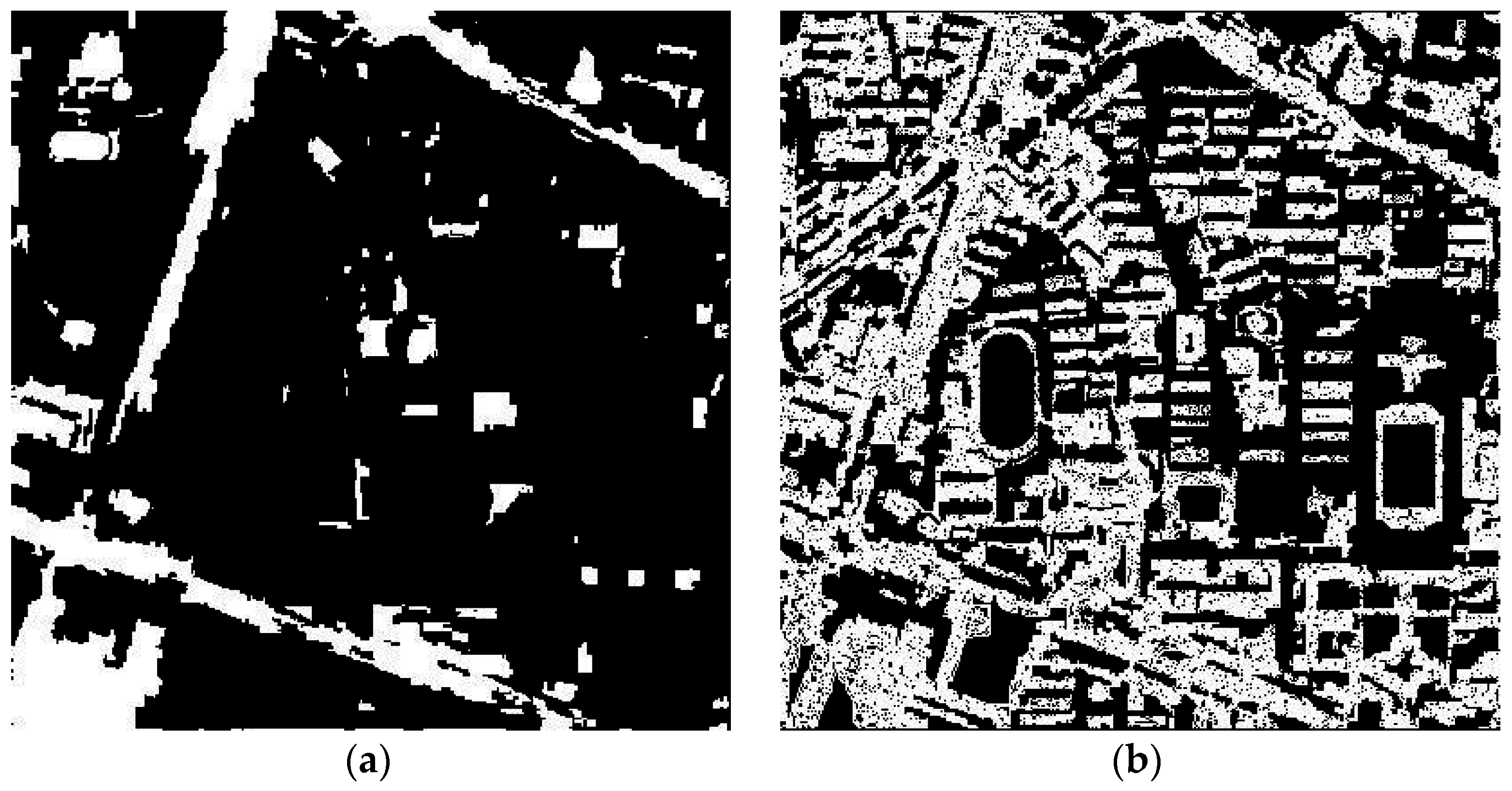
Figure 3.
Interpolated bi-temporal images of the first study area. (a) Acquired by QuickBird in April 2005 (L1); and (b) acquired by IKONOS in July 2009 (L2).
Figure 3.
Interpolated bi-temporal images of the first study area. (a) Acquired by QuickBird in April 2005 (L1); and (b) acquired by IKONOS in July 2009 (L2).

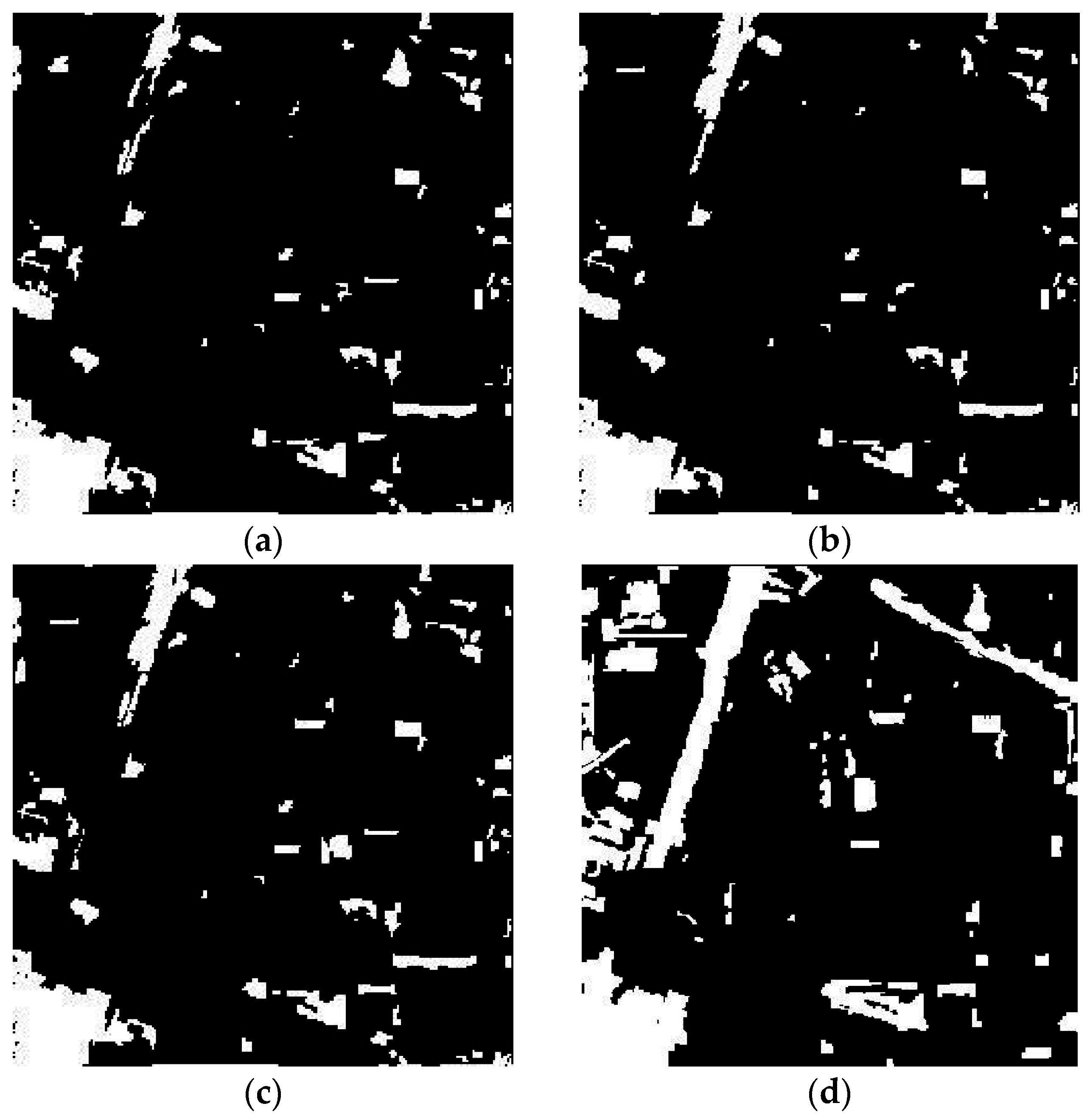
Figure 4.
The change detection maps resulting from: (a) Otsu’s thresholding method, (b) threshold selection by clustering gray levels of boundaries, and (c) k-means clustering (k = 2), compared with (d) the reference image, with L1 as the basis image in the first study area (scale = 100).
Figure 4.
The change detection maps resulting from: (a) Otsu’s thresholding method, (b) threshold selection by clustering gray levels of boundaries, and (c) k-means clustering (k = 2), compared with (d) the reference image, with L1 as the basis image in the first study area (scale = 100).


Figure 5.
Overall errors of change detection with different segmentation scales, with L1 as the basis image in the first study area.
Figure 5.
Overall errors of change detection with different segmentation scales, with L1 as the basis image in the first study area.
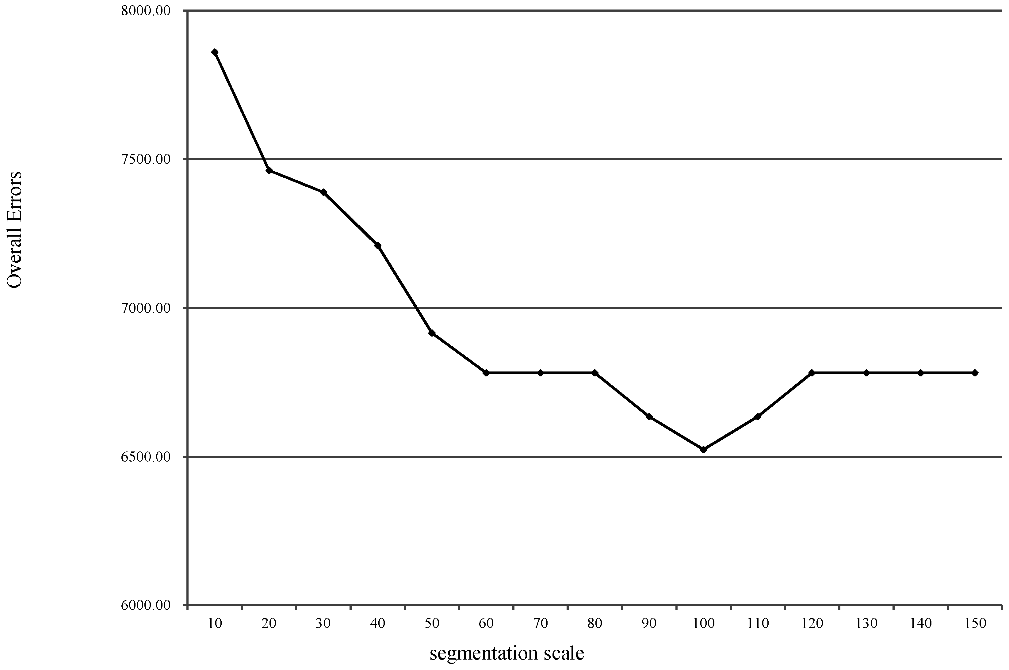
Figure 6.
Overall errors of change detection using different multi-scale fusion thresholds, with L1 as the basis image in the first study area.
Figure 6.
Overall errors of change detection using different multi-scale fusion thresholds, with L1 as the basis image in the first study area.
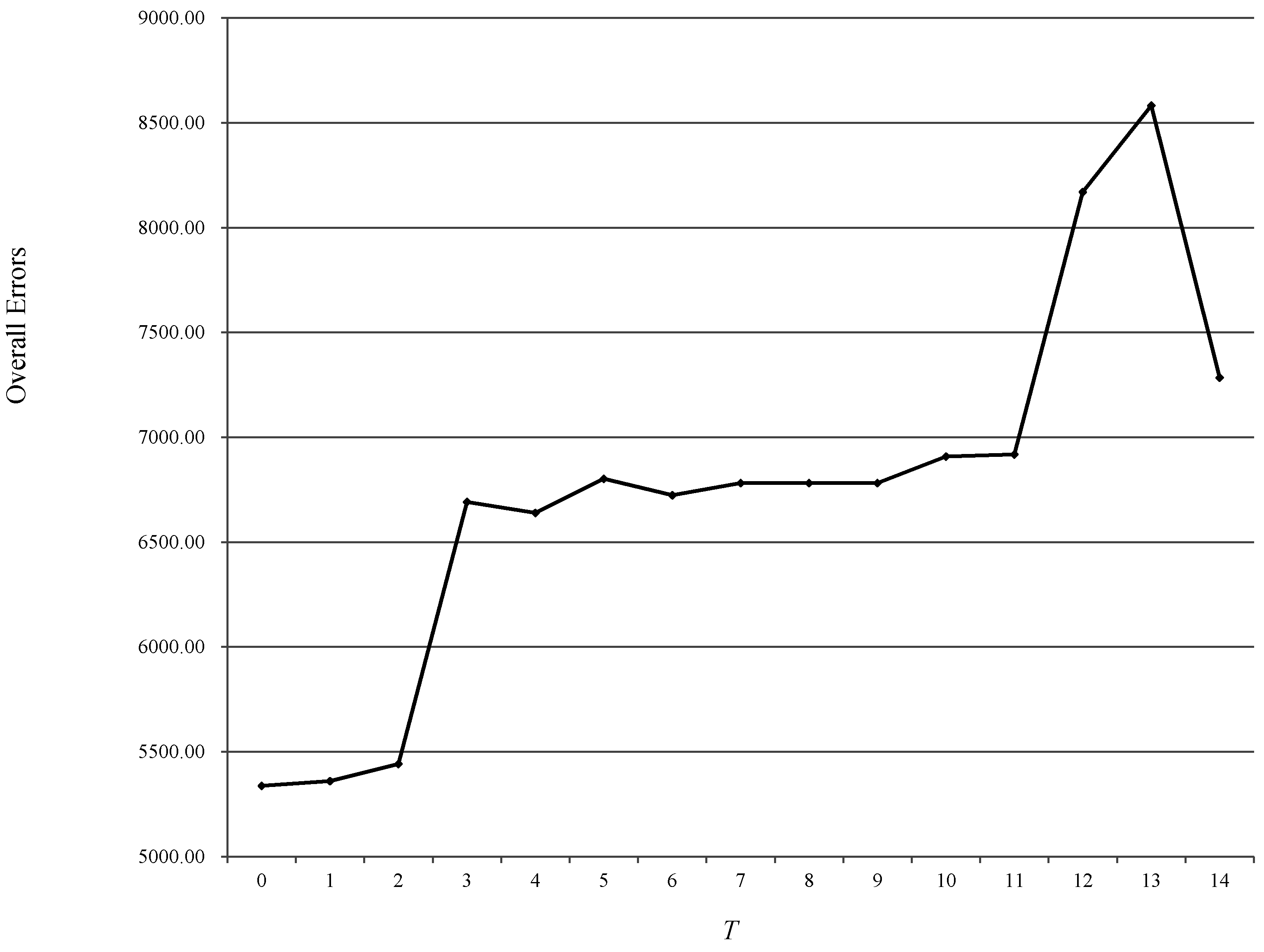
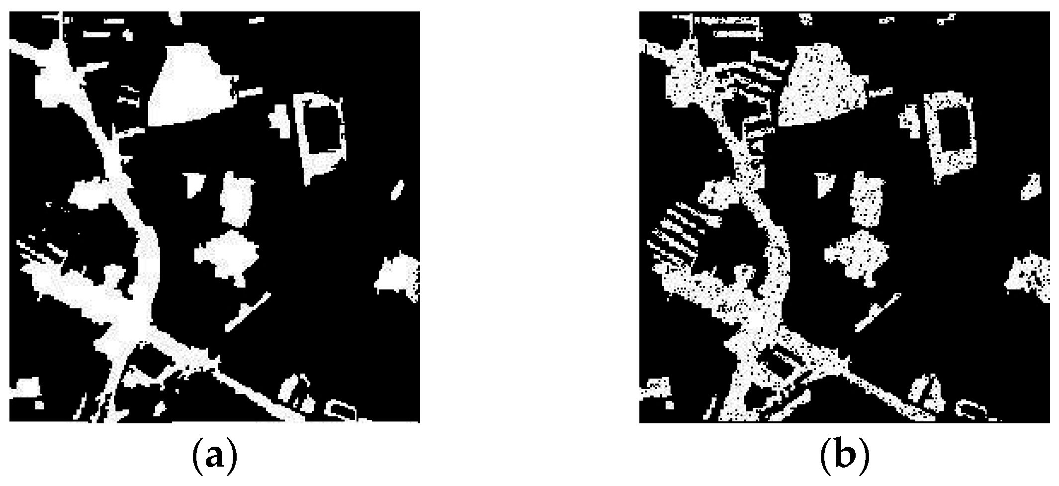
Figure 7.
Change detection maps resulting from (a) the proposed multi-scale k-means method and (b) the method using varying geometric and radiometric properties [35], with L2 as the basis image in the first study area (scale = 100).
Figure 7.
Change detection maps resulting from (a) the proposed multi-scale k-means method and (b) the method using varying geometric and radiometric properties [35], with L2 as the basis image in the first study area (scale = 100).

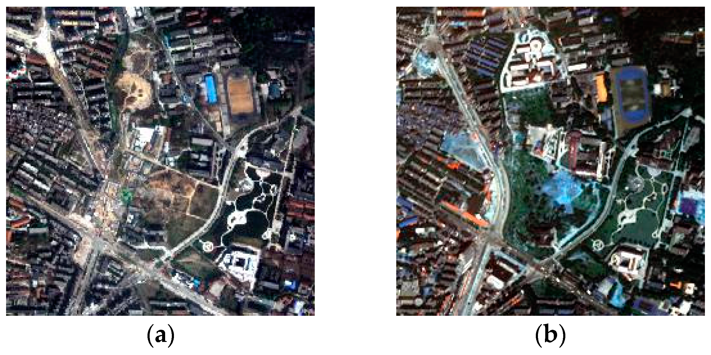
Figure 8.
Degraded bi-temporal images of the first study area: (a) acquired by QuickBird in April 2005 (L1) and (b) acquired by IKONOS in July 2009 (L2).
Figure 8.
Degraded bi-temporal images of the first study area: (a) acquired by QuickBird in April 2005 (L1) and (b) acquired by IKONOS in July 2009 (L2).
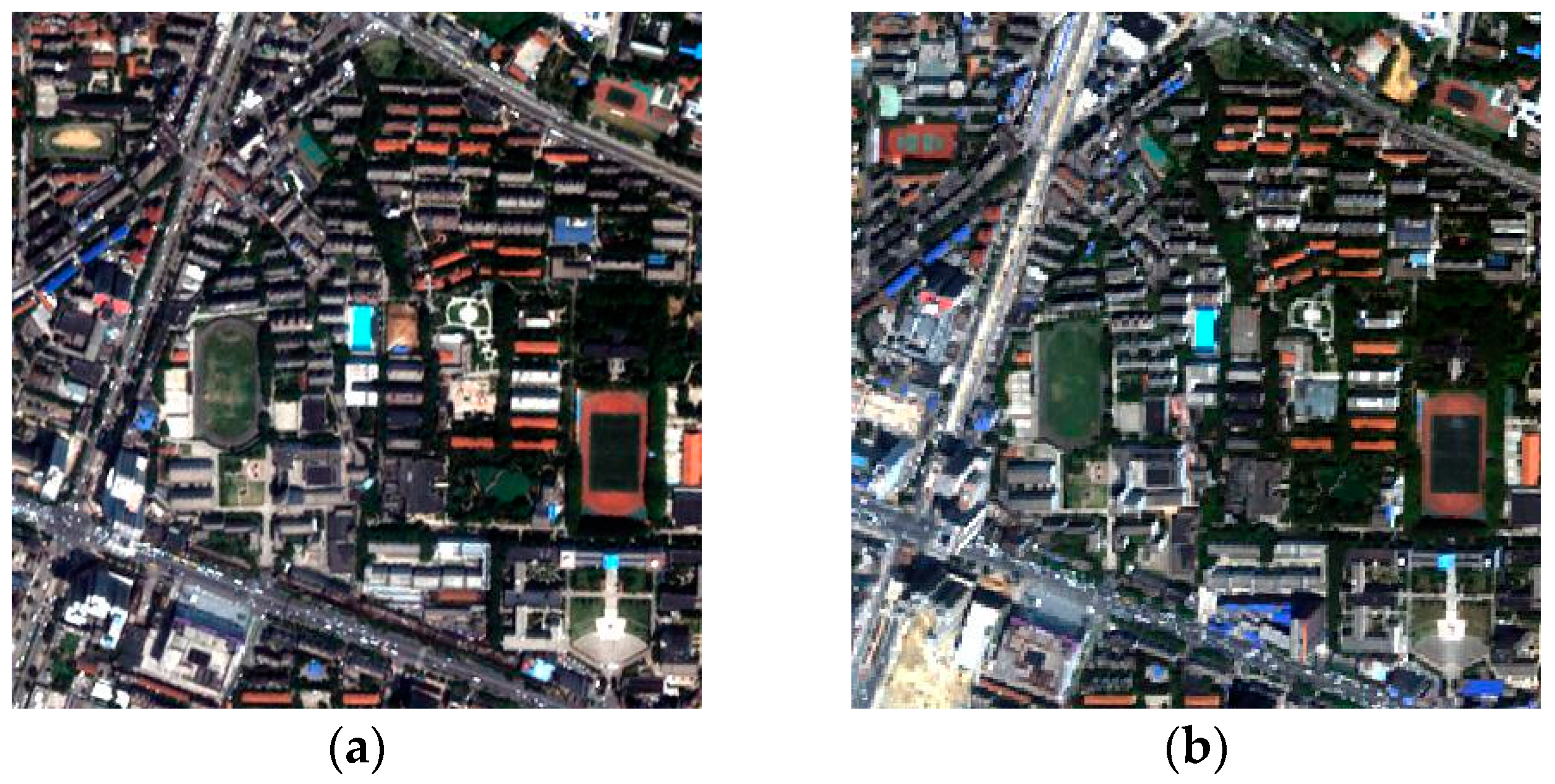
Figure 9.
The change detection maps resulting from (a) Otsu’s thresholding method, (b) threshold selection by clustering gray levels of boundary, and (c) k-means clustering (k = 2), compared with (d) the reference image, with L2 as the basis image in the first study area (scale = 50).
Figure 9.
The change detection maps resulting from (a) Otsu’s thresholding method, (b) threshold selection by clustering gray levels of boundary, and (c) k-means clustering (k = 2), compared with (d) the reference image, with L2 as the basis image in the first study area (scale = 50).

Figure 10.
Overall errors of the change detection with different segmentation scales, with L2 as the basis image in the first study area.
Figure 10.
Overall errors of the change detection with different segmentation scales, with L2 as the basis image in the first study area.
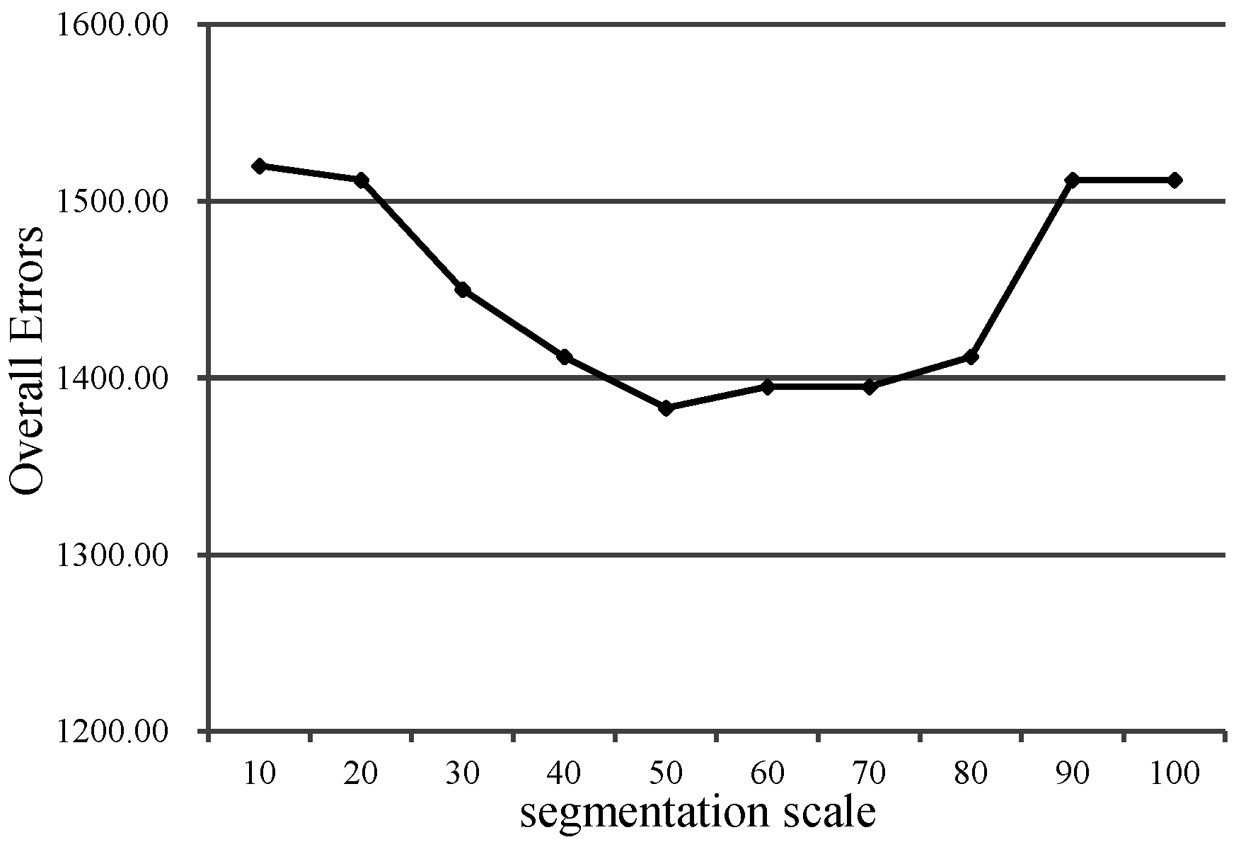
Figure 11.
Change detection maps resulting from (a) the proposed multi-scale k-means method and (b) the method using varying geometric and radiometric properties [35], with L2 as the basis image in the first study area (scale = 50).
Figure 11.
Change detection maps resulting from (a) the proposed multi-scale k-means method and (b) the method using varying geometric and radiometric properties [35], with L2 as the basis image in the first study area (scale = 50).
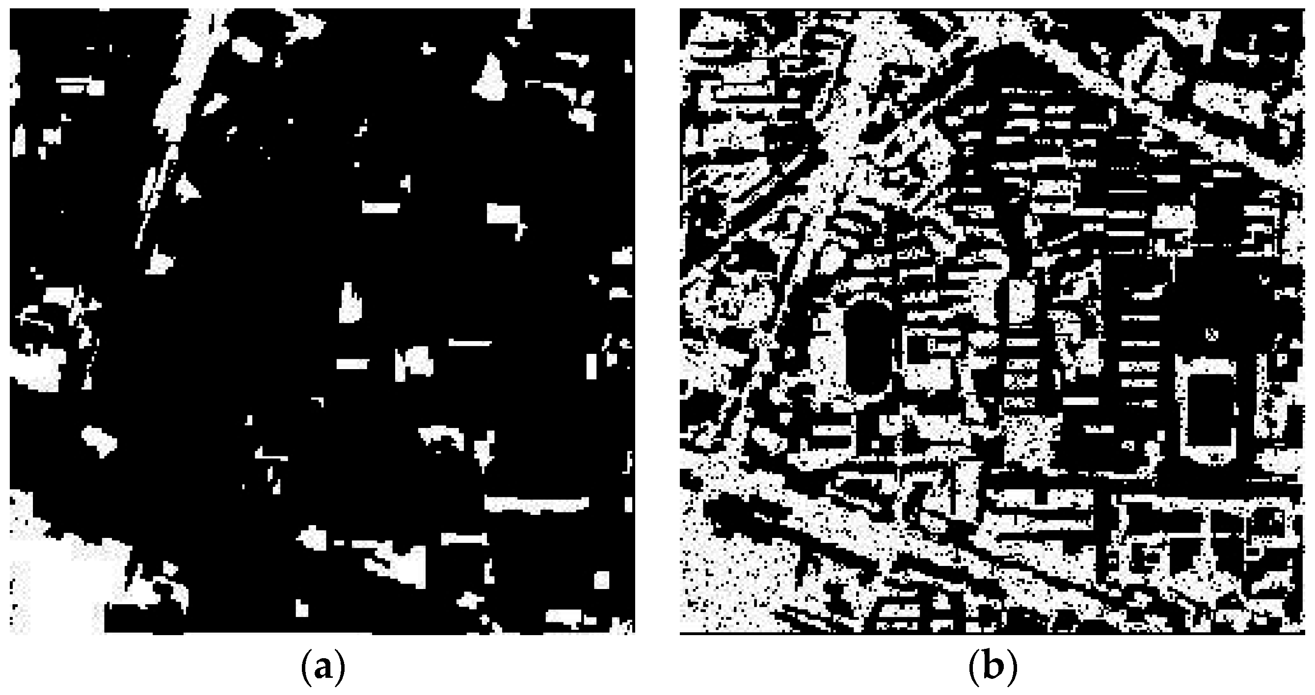
Figure 12.
Preprocessed bi-temporal images of the second study area: (a) acquired by QuickBird in May 2002 (L1) and (b) acquired by IKONOS in July 2009 (L2).
Figure 12.
Preprocessed bi-temporal images of the second study area: (a) acquired by QuickBird in May 2002 (L1) and (b) acquired by IKONOS in July 2009 (L2).

Figure 13.
Change detection maps resulting from: (a) Otsu’s thresholding method, (b) threshold selection by clustering gray levels of boundary, and (c) k-means clustering (k = 2), compared with (d) the reference image, with L2 as the basis image in the second study area (scale = 50).
Figure 13.
Change detection maps resulting from: (a) Otsu’s thresholding method, (b) threshold selection by clustering gray levels of boundary, and (c) k-means clustering (k = 2), compared with (d) the reference image, with L2 as the basis image in the second study area (scale = 50).
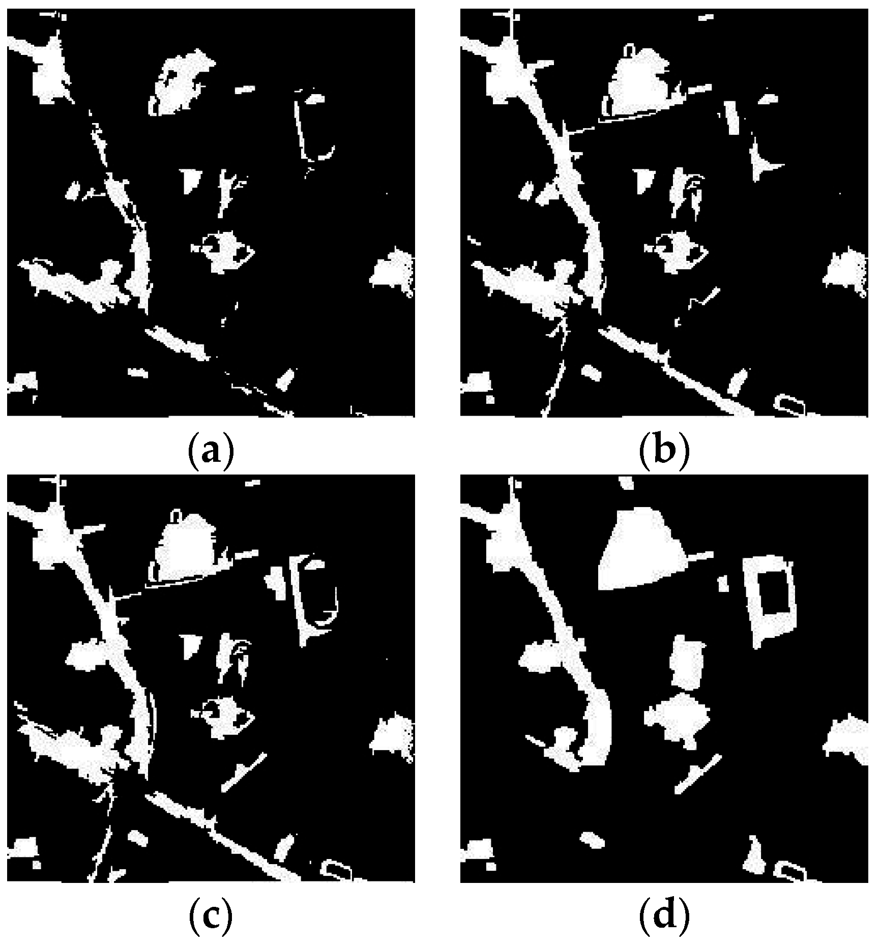
Figure 14.
Change detection maps resulting from (a) the proposed multi-scale k-means method and (b) the method using varying geometric and radiometric properties [35], with L2 as the basis image in the second study area (scale = 50).
Figure 14.
Change detection maps resulting from (a) the proposed multi-scale k-means method and (b) the method using varying geometric and radiometric properties [35], with L2 as the basis image in the second study area (scale = 50).


| Blue Band (um) | Green Band (um) | Red Band (um) | Near Infrared band (um) | Spatial Resolution (nadir, m) | |
|---|---|---|---|---|---|
| QuickBird MS image | 0.45–0.52 | 0.52–0.60 | 0.63–0.69 | 0.76–0.90 | 2.44 |
| IKONOS MS image | 0.445–0.516 | 0.506–0.595 | 0.632–0.698 | 0.757–0.853 | 3.28 |
Table 2.
Comparison between the change detection results of the three thresholding and clustering methods, with L1 as the basis image in the first study area (scale = 100).
| Combination Ratio of Change Maps | False Alarm_Otsu | False Alarm_Edge | False Alarm_K-Means | Missed Alarm_Otsu | Missed Alarm_Edge | Missed Alarm_K-Means | Overall Errors_Otsu | Overall Errors_Edge | Overall Errors_K-Means |
|---|---|---|---|---|---|---|---|---|---|
| 1:9 | 1.47% | 1.52% | 2.04% | 5.57% | 4.88% | 3.65% | 7.04% | 6.39% | 5.69% |
| 2:8 | 1.35% | 1.41% | 1.91% | 5.54% | 4.82% | 3.43% | 6.89% | 6.23% | 5.34% |
| 3:7 | 1.28% | 1.36% | 1.89% | 5.52% | 4.80% | 3.38% | 6.80% | 6.16% | 5.27% |
| 4:6 | 1.24% | 1.31% | 1.66% | 5.38% | 4.76% | 3.24% | 6.62% | 6.07% | 4.90% |
| 5:5 | 1.15% | 1.25% | 1.69% | 5.38% | 4.70% | 2.93% | 6.54% | 5.94% | 4.63% |
| 6:4 | 1.07% | 1.13% | 1.70% | 4.95% | 4.64% | 2.88% | 6.02% | 5.77% | 4.58% |
| 7:3 | 0.98% | 1.05% | 1.72% | 4.73% | 4.34% | 2.86% | 5.70% | 5.39% | 4.59% |
| 8:2 | 0.96% | 1.08% | 1.70% | 4.55% | 4.20% | 2.77% | 5.51% | 5.27% | 4.47% |
| 9:1 | 0.94% | 1.04% | 1.66% | 4.16% | 3.86% | 2.42% | 5.10% | 4.89% | 4.08% |
Table 3.
Comparison between the change detection results of the single-scale and multi-scale proposed method, with L1 as the basis image in the first study area.
| False Alarms_Kmeans | Missed Alarms_Kmeans | Overall Error_Kmeans | |
|---|---|---|---|
| The optimal scale = 100 | 1.66% | 2.42% | 4.08% |
| Multi-scale: 10, 20, …, 150 | 2.53% | 0.81% | 3.33% |
Table 4.
Comparison between the change detection results of the three thresholding and clustering methods, with L2 as the basis image in the first study area (scale = 50).
| Combination Ratio of Change Maps | False Alarm_Otsu | False Alarm_Edge | False Alarm_K-means | Missed Alarm_Otsu | Missed Alarm_Edge | Missed Alarm_K-means | Overall Errors_Otsu | Overall Errors_Edge | Overall Errors_K-means |
|---|---|---|---|---|---|---|---|---|---|
| 1:9 | 0.10% | 0.10% | 0.13% | 1.20% | 1.09% | 0.73% | 1.30% | 1.19% | 0.86% |
| 2:8 | 0.10% | 0.10% | 0.13% | 1.28% | 1.11% | 0.74% | 1.38% | 1.21% | 0.87% |
| 3:7 | 0.10% | 0.10% | 0.14% | 1.28% | 1.13% | 0.80% | 1.38% | 1.23% | 0.93% |
| 4:6 | 0.12% | 0.11% | 0.14% | 1.42% | 1.28% | 0.80% | 1.53% | 1.39% | 0.94% |
| 5:5 | 0.12% | 0.10% | 0.14% | 1.47% | 1.30% | 0.81% | 1.58% | 1.40% | 0.94% |
| 6:4 | 0.12% | 0.10% | 0.14% | 1.50% | 1.31% | 0.94% | 1.62% | 1.41% | 1.07% |
| 7:3 | 0.12% | 0.11% | 0.14% | 1.52% | 1.33% | 1.02% | 1.64% | 1.44% | 1.16% |
| 8:2 | 0.13% | 0.09% | 0.17% | 1.52% | 1.39% | 1.06% | 1.65% | 1.48% | 1.23% |
| 9:1 | 0.13% | 0.10% | 0.17% | 1.52% | 1.38% | 1.09% | 0.00% | 1.48% | 1.26% |
Table 5.
Comparison between the change detection results of the single-scale and multi-scale proposed method, with L2 as the basis image in the first study area.
| False Alarms_Kmeans | Missed Alarms_Kmeans | Overall Errors_Kmeans | |
|---|---|---|---|
| The optimal scale = 50 | 0.13% | 0.73% | 0.86% |
| Multi-scale: 10, 20, …, 100 | 0.15% | 0.52% | 0.67% |
Table 6.
Comparison between the change detection results of the three thresholding and clustering methods, with L2 as the basis image in the second study area (scale = 50).
| Combination Ratio of Change Maps | False Alarm_Otsu | False Alarm_Edge | False Alarm_K-Means | Missed Alarm_Otsu | Missed Alarm_Edge | Missed Alarm_K-Means | Overall Errors_Otsu | Overall Errors_Edge | Overall Errors_K-Means |
|---|---|---|---|---|---|---|---|---|---|
| 1:9 | 0.30% | 0.28% | 0.36% | 1.66% | 1.52% | 1.00% | 1.95% | 1.80% | 1.37% |
| 2:8 | 0.31% | 0.38% | 0.42% | 1.67% | 1.51% | 1.02% | 1.98% | 1.89% | 1.44% |
| 3:7 | 0.35% | 0.39% | 0.40% | 1.68% | 1.50% | 1.07% | 2.03% | 1.90% | 1.47% |
| 4:6 | 0.35% | 0.38% | 0.40% | 1.72% | 1.53% | 1.08% | 2.07% | 0.00% | 1.48% |
| 5:5 | 0.36% | 0.29% | 0.35% | 1.76% | 1.67% | 1.14% | 2.11% | 1.95% | 1.50% |
| 6:4 | 0.36% | 0.36% | 0.40% | 1.82% | 1.70% | 1.10% | 2.17% | 2.06% | 1.50% |
| 7:3 | 0.36% | 0.35% | 0.40% | 1.84% | 1.74% | 1.15% | 2.20% | 2.09% | 1.54% |
| 8:2 | 0.38% | 0.35% | 0.38% | 1.89% | 1.77% | 1.20% | 2.27% | 2.12% | 1.58% |
| 9:1 | 0.44% | 0.34% | 0.39% | 1.94% | 1.81% | 1.22% | 2.38% | 2.16% | 1.61% |
Table 7.
Comparison between the change detection results of the single-scale and multi-scale proposed method, with L2 as the basis image in the second study area.
| False Alarms_Kmeans | Missed Alarms_Kmeans | Overall Errors_Kmeans | |
|---|---|---|---|
| The optimal scale = 50 | 0.36% | 1.00% | 1.37% |
| Multi-scale: 10, 20, …, 100 | 0.55% | 0.22% | 0.84% |
© 2017 by the authors. Licensee MDPI, Basel, Switzerland. This article is an open access article distributed under the terms and conditions of the Creative Commons Attribution (CC BY) license ( http://creativecommons.org/licenses/by/4.0/).
Share and Cite
MDPI and ACS Style
Tang, Y.; Zhang, L. Urban Change Analysis with Multi-Sensor Multispectral Imagery. Remote Sens. 2017, 9, 252. https://doi.org/10.3390/rs9030252
AMA Style
Tang Y, Zhang L. Urban Change Analysis with Multi-Sensor Multispectral Imagery. Remote Sensing. 2017; 9(3):252. https://doi.org/10.3390/rs9030252
Chicago/Turabian StyleTang, Yuqi, and Liangpei Zhang. 2017. "Urban Change Analysis with Multi-Sensor Multispectral Imagery" Remote Sensing 9, no. 3: 252. https://doi.org/10.3390/rs9030252
Note that from the first issue of 2016, this journal uses article numbers instead of page numbers. See further details here.