Article

Optimising Phenological Metrics Extraction for Different Crop Types in Germany Using the Moderate Resolution Imaging Spectrometer (MODIS)

1
Department of Computational Landscape Ecology, Helmholtz-Centre for Environmental Research—UFZ, Leipzig 04315, Germany
2
Department of Remote Sensing, Institute of Geography and Geology, University of Würzburg, 97074 Würzburg, Germany
*
Author to whom correspondence should be addressed.
Remote Sens. 2017, 9(3), 254; https://doi.org/10.3390/rs9030254
Submission received: 2 January 2017 / Revised: 24 February 2017 / Accepted: 6 March 2017 / Published: 9 March 2017

Abstract

:
Phenological metrics extracted from satellite data (phenometrics) have been increasingly used to access timely, spatially explicit information on crop phenology, but have rarely been calibrated and validated with field observations. In this study, we developed a calibration procedure to make phenometrics more comparable to ground-based phenological stages by optimising the settings of Best Index Slope Extraction (BISE) and smoothing algorithms together with thresholds. We used a six-year daily Moderate Resolution Imaging Spectrometer (MODIS) Normalized Difference Vegetation Index (NDVI) time series and 211 ground-observation records from four major crop species (winter wheat/barley, oilseed rape, and sugar beet) in central Germany. Results showed the superiority of the Savitzky–Golay algorithm in combination with BISE. The satellite-derived senescence dates matched ripeness stages of winter crops and the dates with maximum NDVI were closely related to the field-observed heading stage of winter cereals. We showed that the emergence of winter crops corresponded to the dates extracted with a threshold of 0.1, which translated into 8.89 days of root-mean-square error (RMSE) improvement compared to the standard threshold of 0.5. The method with optimised settings and thresholds can be easily transferred and applied to areas with similar growing conditions. Altogether, the results improve our understanding of how satellite-derived phenometrics can explain in situ phenological observations.

Graphical Abstract

1. Introduction

Crop phenology is characterised by a set of growth stages, such as emergence, flowering, and fruit ripening. These phenological events contain essential information for the adjustment of agronomic practices (fertilisation, irrigation, and crop protection). Such information on crop phenology is also one of the key requirements for sustainable farming [1] and can improve crop productivity estimations, e.g., as base layers for agricultural monitoring services (such as the crop calendar of the Crop Monitor within the Group on Earth Observations Global Agricultural Monitoring Initiative). Thus, accurate, spatially distributed information on crop phenology on large scales is crucial for meeting the globally increasing demand for food and water resources [2].
Remote sensing, particularly the use of optical satellite imagery, has become an emerging tool for monitoring phenological events of crops at regional to national scales [3,4,5]. Sensors, such as the Advanced Very High Resolution Radiometer (AVHRR) and the Moderate Resolution Imaging Spectrometer (MODIS), provide daily vegetation index (VI) observations for evaluating phenological characteristics, among others in agricultural areas [6,7]. VIs are indicators of the abundance of different leaf components (pigments, water, nitrogen etc.) that are responsible for the absorption of radiation [8]. Therefore, changes in canopy biophysical properties are reflected in VI evolution over the growing season of crops [7]. The increase and decrease of VI during crop growth and senescent periods are mainly due to changes of leaf area index, the relationship between chlorophyll and other pigments together with water content [9]. For cereals, VIs usually reach their maximum at the late booting to the beginning of heading stage after the last leaf (e.g., flag leaf) is fully unfolded [10,11,12]. During this period of time, the development of all shoots (main stem and tillers) on the same plant also gradually synchronises [13].
As VI time series are usually affected by noise caused by clouds, atmospheric constituents and varying viewing geometries of the sensor, several compositing algorithms have been developed for noise reduction. The maximum value composite (MVC) method is widely used to minimize negatively biased noise by selecting the highest VI value to represent a certain period (8–16 days) [14]. However, the use of MVC methods can result in unnecessary loss of data when there are several noise-free VI values within one compositing period. The Best Index Slope Extraction (BISE) algorithm [15] has advantages over MVC as it potentially retains more observations which contain true vegetation signals. BISE could also eliminate data transmission errors which cause abnormally high VI values. The performance of this method can be optimised by varying a so-called sliding period. The sliding period defines a time window within which changes in VI time series, i.e., phenological variability, should be accepted. This time window also determines how many true VI measurements (i.e., not hampered by clouds) can be expected. Despite of its importance, we did not find a systematic assessment on the sensitivity of sliding periods for crop phenology monitoring in the literature.
Many different smoothing and model fitting methods have been applied on composited products to construct high-quality VI time series [16,17,18]. Each method has its own advantages as well as limitations. In contrast to model fitting, filtering algorithms tend to require fewer parameters and can better preserve irregular intra-seasonal VI curves, which are typically observed in agricultural fields with more than one growing season in a year [19]. More recently, Zhao et al. [20] compared double logistic functions [21] and the Savitzky–Golay filter (SG) [17] to detect phenological stages (phenostages) of summer crops in the United States. Nevertheless, to our knowledge, comprehensive comparisons of smoothing methods for crop phenology mapping over agricultural areas and multiple years, i.e., including crop rotations, have not been published yet.
Calibration and validation of satellite-derived crop phenology, i.e., investigations of deviations between phenometrics and field-observed phenostages, are not straightforward and are rarely addressed. This situation is in large part due to a lack of dense and evenly distributed in situ data, and the difficulties of matching ground observations to the satellite-derived phenological metrics (phenometrics). Typically, thresholds, such as the half maximum or maximum slope, have been used to retrieve general vegetation seasonal metrics [7,21]. However, some of these metrics, for example for the onset of greening and senescence, are unable to represent specific agronomic stages. Some limited their studies to only one stage of one crop due to lack of available data [22,23,24]. Only a few studies have detected specific agronomic stages from satellite-derived time-series data [10,25,26]. Although high estimation accuracies were achieved, their two-step filtering model was more suitable for areas where deviations of phenostages were relatively small between different years and different test sites. Besides, the settings of the models needed to be re-adjusted for other study areas and for different crops (maize and soybean). Therefore, it is necessary to have a more general and transferrable approach to define crop phenometrics associated with the specific agronomic stages.
In Germany, crop rotation is dominated by winter cereals, oilseed rape, sugar beet, maize and potato, which results in unevenly distributed growing seasons. Phenological data of these species recorded by the German Meteorological Service (DWD) have been applied to investigate crop–weather relationships and model-based crop phenology [27], but have not yet been used for validation of satellite-derived phenometrics. Thus, the goal of this study is:
(1).
to systematically optimise the derivation of phenometrics from MODIS Normalized Difference Vegetation Index (NDVI) time series in terms of the BISE sliding period, smoothing algorithms and thresholds for four major crops (winter wheat, winter barley, oilseed rape, and sugar beet) in central Germany;
(2).
to calibrate and validate satellite-derived phenometrics with field-observed phenostages of different crop types (e.g., emergence, heading, and yellow ripeness for winter cereals; emergence and full ripeness for oilseed rape; emergence for sugar beet).

2. Materials and Methods
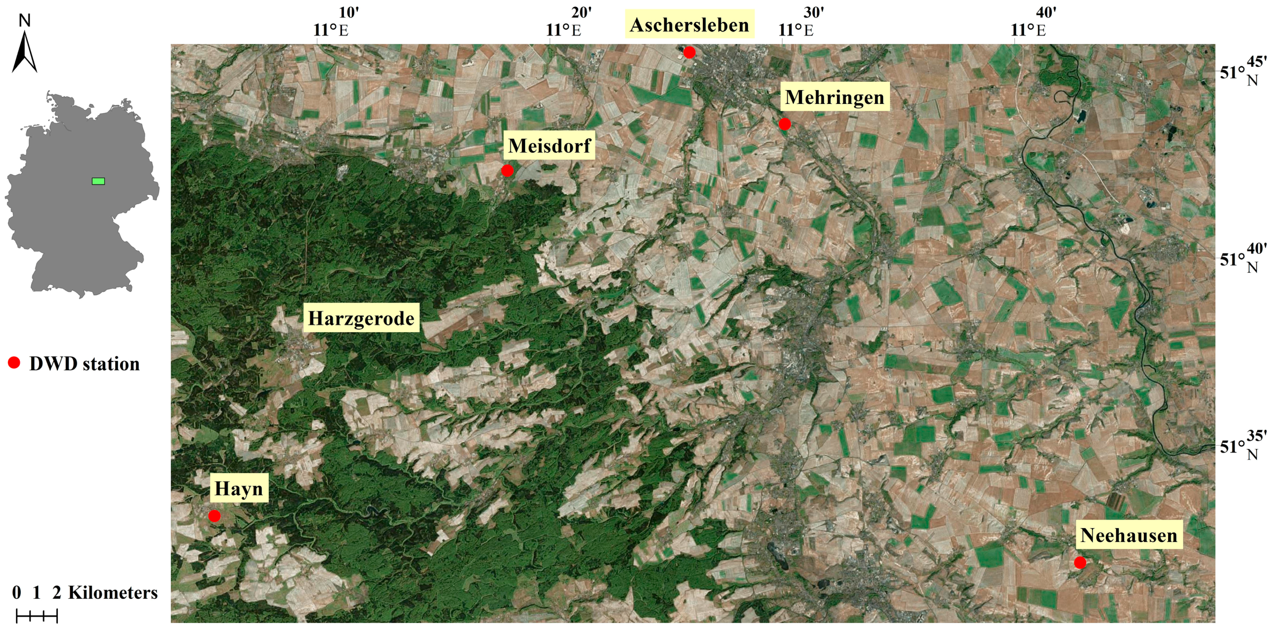
2.1. Study Area

The study site is located in Saxony-Anhalt, central Germany (Figure 1). Mean air temperature is 9.44 °C and annual precipitation is 600.38 mm (data from DWD for the years 2010–2013). Crop fields with average size of around 9 ha cover almost 56% of the total 1225 km2. Mean ground elevation of most agricultural areas is around 200 m, except for around 15% of the fields which are located in the Harz Mountains. Major crops were winter wheat (49.2%), winter oilseed rape (12.4%), winter barley (10.1%), sugar beet (3.9%), and silage maize (3.8%) (average percentages of total crop area for 2010–2014). In general, the sowing dates of the summer crops ranged from early April to mid-May, depending on weather and soil moisture conditions. The winter crops were normally planted between late August and late October and emerged before winter.

2.2. MODIS Data

We used the MODIS Aqua daily data (MYD09GQ L2G, Collection 5) at a 250-m spatial resolution from 2009 to 2015. It offers the atmospherically corrected surface reflectance data for the red band (RED; 620–670 nm) and the near infrared band (NIR; 841–876 nm), which were used to derive NDVI [28] as given in the following equation:
NDVI = (NIR − RED)/(NIR + RED).
MODIS Terra data was not selected for this study, because Aqua NDVI values were shown to have relatively high correlations with in situ NDVI and smaller bidirectional reflectance distribution function effects [29].
The MODIS Aqua daily 500-m snow product (MYD10A1, Collection 5) was used to build masks for filtering snow and cloud contamination from Aqua NDVI data. This product contains a binary-coded snow cover map, cloud state and quality assessment information. The dataset was first resampled to 250 m and then the corresponding snow and cloud state were used only for pixels assessed to be of “good quality” [30].

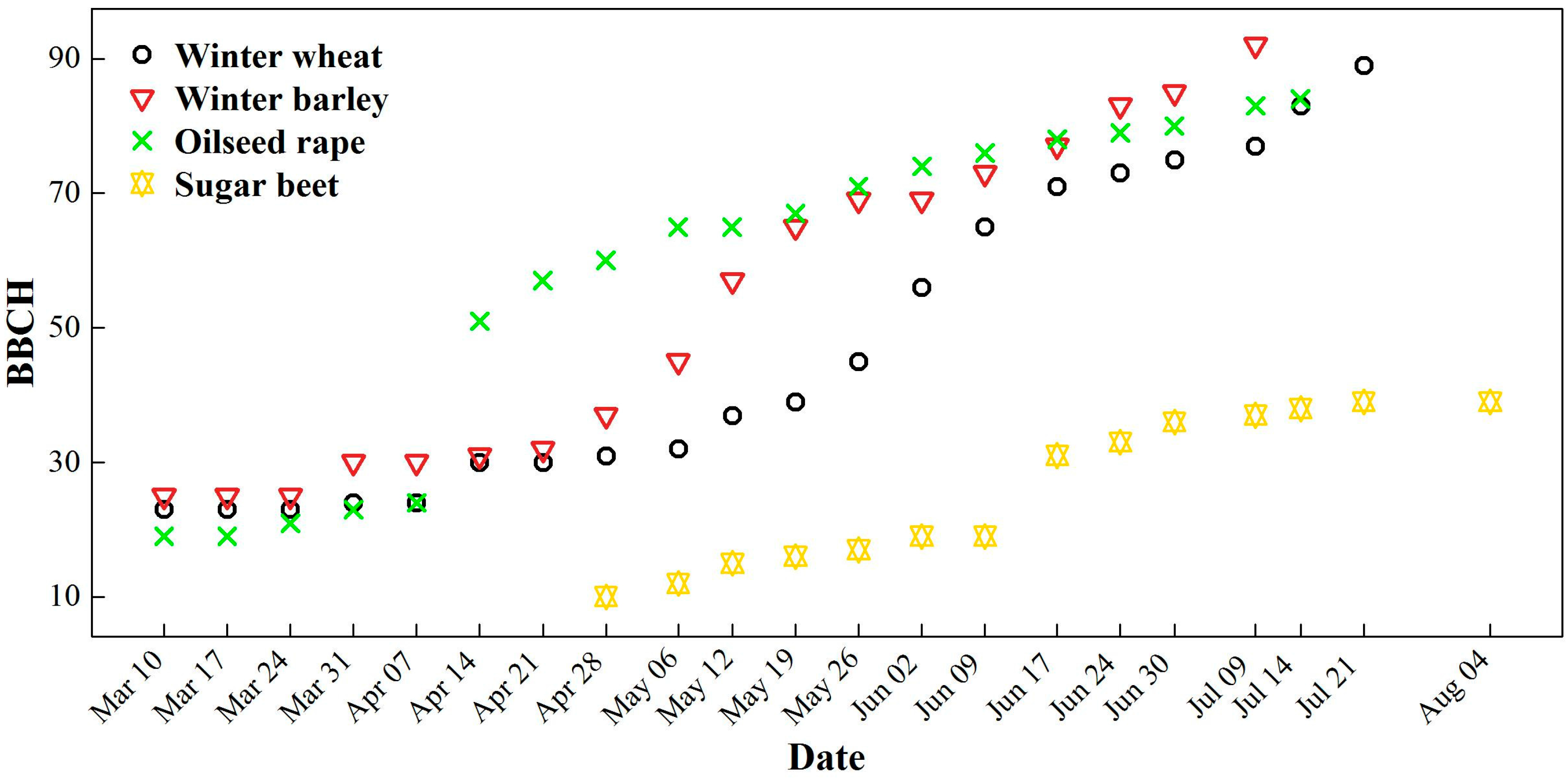
2.3. Field Phenology Data and Ancillary Data

Ground truth data was obtained from five DWD stations shown in Figure 1. The phenostages of major crops which were used to evaluate phenometrics are listed in Table 1. DWD records were collected by a network of voluntary observers within a radius of 1.5–2 km (maximum 5 km) of the stations [31]. According to the guidelines for observers, crops are observed from sowing to harvest in one and the same plot/field which must not differ more than 50 m in altitude from the mean altitude of the observation station. A phase is considered to have begun when approximately 50% of the plants in the field under observation have reached the corresponding stage of development. After removal of obviously questionable records (e.g., observations assigned to the wrong season or those where different phenostages co-occurred on the same date for the same site and year), the number of records for each crop species and phenostage varied every year.
In 2014 and 2015, we additionally recorded Biologische Bundesanstalt für Land- und Forstwirtschaft, Bundessortenamt und CHemische Industrie (BBCH) stages for four species (winter wheat, winter barley, oilseed rape, and sugar beet) from Aschersleben to Harzgerode every week (Figure 1 and Figure 2). In total, we monitored 41 fields, of which 35 fields were in the relatively flat region (elevation around 200 m) and 6 fields were in the mountain region (elevation around 400 m). One BBCH code was assigned according to the growth stage for the majority of plant species within each field. Afterwards, these phenological records from our own field measurements (hereafter referred to as UFZ data) were transformed to DWD phenology standard (Ekko Bruns, personal communication, July 2014).
Crop maps covering the entire study area were available from 2010 to 2014 (Detlef John, personal communication, 2015). These maps contained information on field boundaries and crop types. We identified approximately 500 fields within which there was at least one homogeneous MODIS pixel and one of four targeted crops was grown. The average size of these identified fields was 48.6 ha, with a minimum of 13.3 ha. In total, we extracted about 1500 homogeneous MODIS pixels for each year. These crop maps were also used to locate fields with certain crops around DWD phenological stations. We selected fields with homogeneous MODIS pixels within a 3-km radius of corresponding stations for each crop for further analysis (calibration and validation).

2.4. Phenometrics Extraction

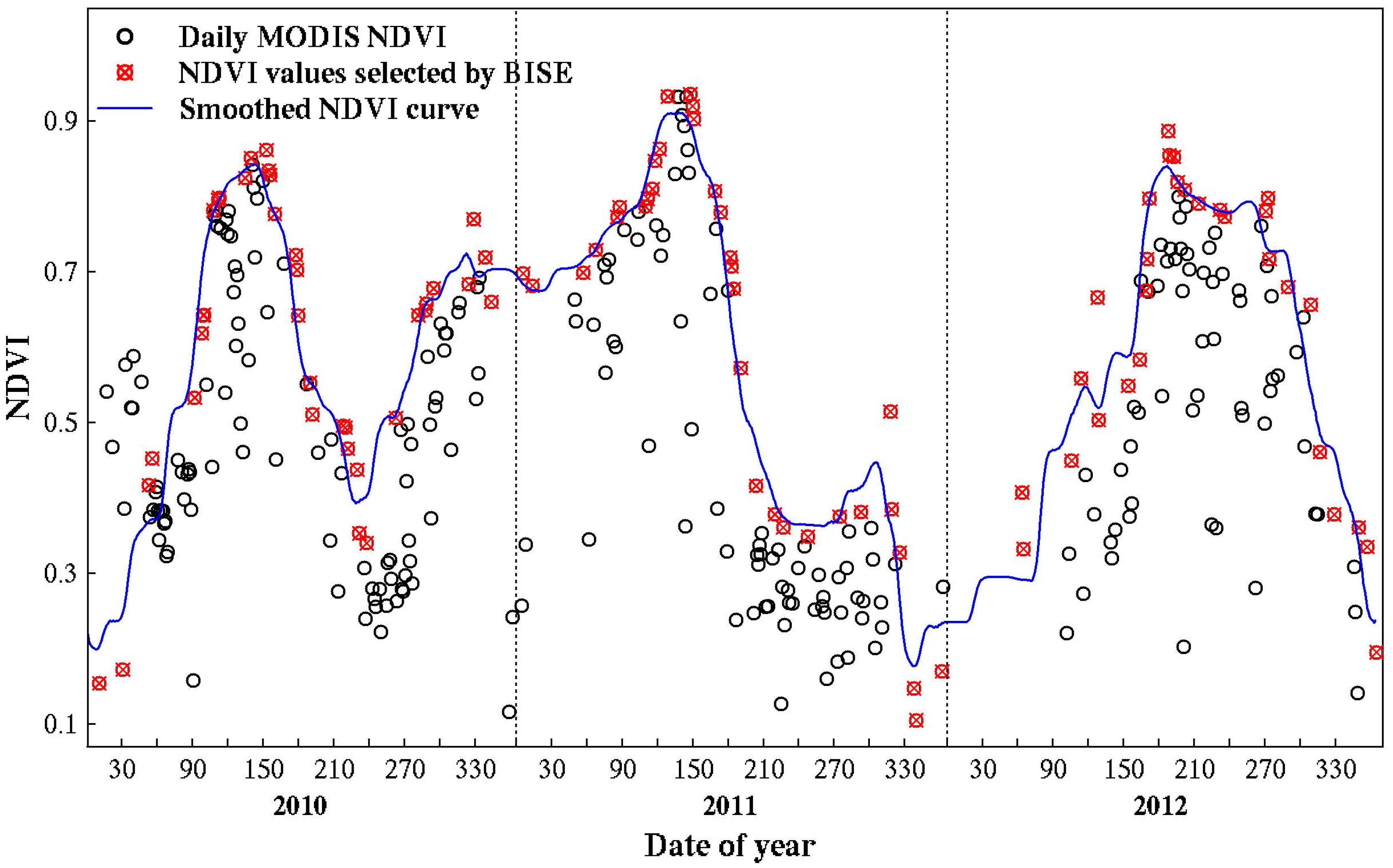
2.4.1. NDVI Time-Series Construction

We used the adapted BISE algorithm to remove remaining undesired data noise from MODIS NDVI time series on a pixel-by-pixel basis, using the ‘phenex’ R package [33]. This algorithm searches from the first date of the NDVI time-series forward and accepts a NDVI increase if the rate-of-change is smaller than a threshold called growth factor. A NDVI decrease will only be accepted if there is no NDVI observation in a pre-defined period of time, called sliding period, which has a value larger than 20% of the difference between the first low value and the previous high value. In this study, we set the growth factor to 0.1 so that the maximal NDVI increase per day was limited to 10%. NDVI time-series will retain too much noise if an excessively short sliding period is chosen and be too smooth to record important changes when an excessively long sliding period is used. Therefore, to reconstruct high-quality NDVI time series, the sliding period needs to be correctly estimated. Another parameter of BISE called cycle value determines whether the end of the NDVI time series is combined with its beginning or not, in order to correctly select NDVI values on the edge of the original NDVI time series. In an agricultural context, however, crop rotation is mostly the decision of individual farmers. Therefore, more original NDVI values were stacked before and after one full phenological cycle for each pixel. Taking into account the complexity of winter and summer crops growing in this region, 3-year NDVI profiles were built (Figure 3). NDVI values of less than 0.1 were identified as soil background and removed before applying BISE. Afterwards, four different smoothly interpolating methods were applied to MODIS NDVI values selected by BISE: fast Fourier transform (FFT), SG [17,34], linear and spline interpolation.

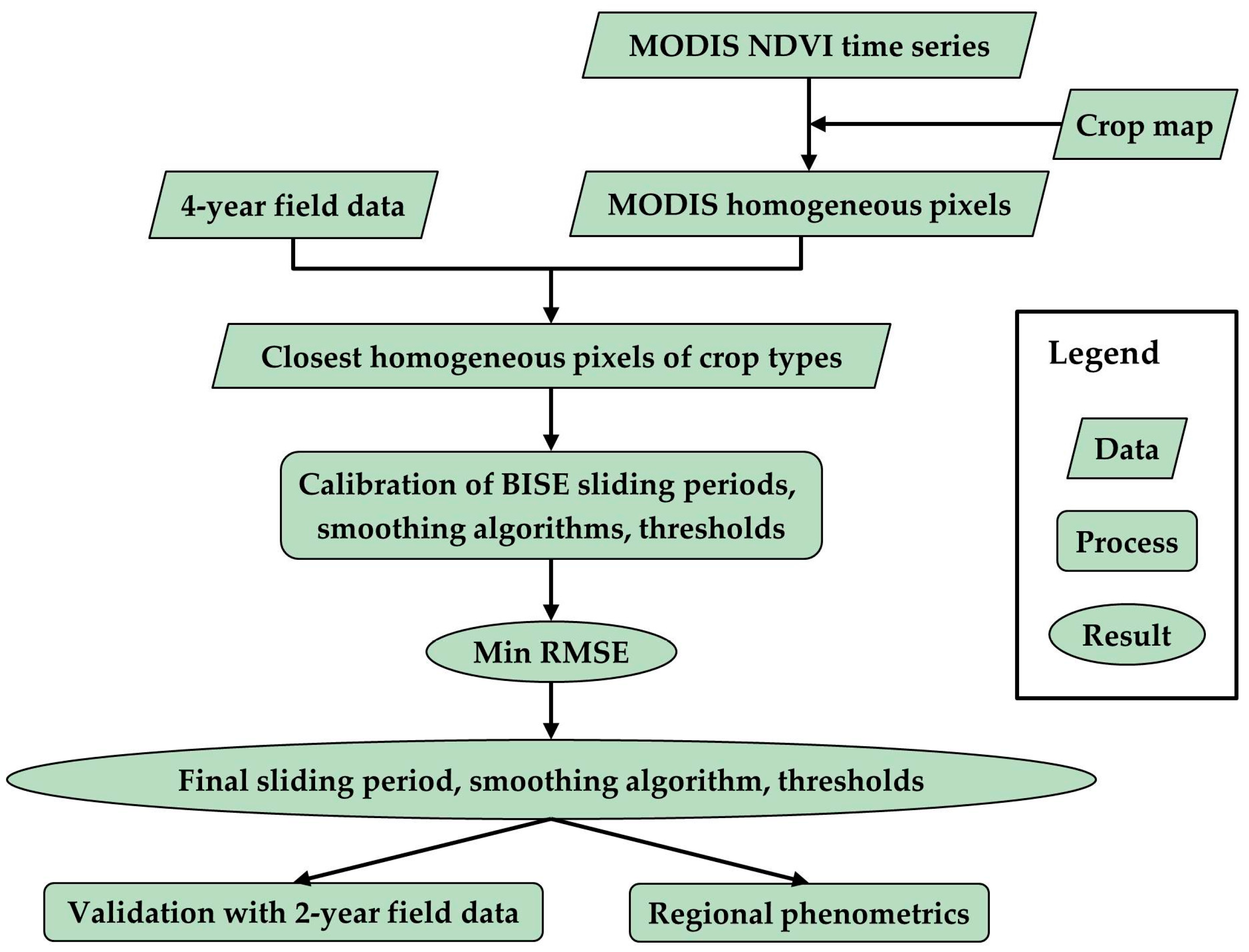
2.4.2. Calibration and Validation of the Phenometrics

In order to extract accurate phenostages comparable to field observations, three questions needed to be answered. Firstly, as BISE is very sensitive to the length of the sliding period, what would be a suitable sliding period for MODIS? Secondly, which is the best smoothing method combined with BISE for phenometrics extraction in our study area? Thirdly, which magnitude of local thresholds for crops should be used to identify certain phenostages? The local threshold is defined such that a phenostage is reached when smoothed NDVI reaches a certain proportion between minimum and maximum of a part of the smoothed NDVI curve. Before calculating phenometrics for the entire study area, we optimised the sliding period and thresholds, and determined the best smoothing method among all four using DWD and UFZ data in the years 2010–2012 and 2014 (Figure 4). In this way, we could rather evenly distribute DWD and UFZ data into calibration and validation. For each smoothing algorithm, the sliding period was iterated from 15 to 35 days, together with the local thresholds from 0 to1 with a step size of 0.01. Specifically, for SG, the iteration process was conducted by iterating possible combinations of two parameters: (1) degree of polynomial fitting (d) in the range of 2–4; and (2) middle width of moving window (m) between 4 and 7. As for FFT, we limited the smoothing intensity of FFT from 1 to 3.
In addition, we set constraints for a smoothed NDVI time series according to the crop calendar as follows:
  • smoothed maximal NDVI cannot occur within 60 days of start and end of one calendar year;
  • the green-up of sugar beet cannot occur after Julian date 195 of one calendar year (around mid-July);
  • senescence cannot occur before Julian date 135 of one calendar year (around mid-May);
  • for the green-up of winter crops, smoothed minimum NDVI should be searched only from Julian date 220 to 280 (mid-July to early October), and smoothed maximum NDVI cannot occur in December.
Due to noisy satellite data during the winter season, we used DWD sowing dates (2010–2015) of winter crops to define the fourth constraint. Throughout the NDVI time-series, we defined the green-up as the beginning of emergence for all targeted crops, the Julian date with smoothed maximal NDVI as the beginning of heading and the senescence as the beginning of yellow ripeness for cereals and as the beginning of full ripeness for oilseed rape. Fields with homogeneous MODIS pixels closest to the DWD stations were chosen to compare with field data in the calibration procedure. If there were two or more pixels within a selected field, then the median value was used. In total, 150 phenostage data from 74 fields (29 fields for winter wheat, 13 for winter barley, 23 for oilseed rape, and 9 for sugar beet) were included in this calibration. The validation dataset comprised 61 phenostage data from 30 fields (17 fields for winter wheat, 4 for winter barley, 5 for oilseed rape, and 4 for sugar beet) in 2013 and 2015. The root-mean-square error (RMSE) for all targeted phenostages was calculated between field data and MODIS-derived phenostages. For each smoothing method, settings including local thresholds and the sliding period were optimised on the calibration dataset. At the end, the method with lowest RMSE of the validation was chosen for calculating phenometrics across the whole study area.

3. Results

3.1. Method Comparison and Parameter Calibration

Based on RMSE of the calibration using 4-year field data, the SG filter performed best followed by the FFT and linear interpolation (Table 2). The optimised sliding periods of these methods were all within 3–4 weeks, and local thresholds for each phenometrics were also within very narrow ranges. The threshold values for green-up of winter crops were between 0.1 and 0.17, and those of sugar beet were between 0.26 and 0.3. With the (d,m) combination of (2,5), respectively, for SG, we also found that the sliding periods in the range of 20–35 scored the highest RMSE values (12.76–14.35 days) for calibration. Since the RMSE of the validation using SG was the smallest compared to the other three methods, SG with the optimised settings and thresholds in Table 2 were then used for phenometrics calculation of the entire study area.

3.2. Calibration Results Using the Savitzky-Golay Filter

In general, the senescence and heading of winter cereals achieved higher calibration accuracy than the green-up stage (Table 3). Compared to 4-year field data, the smallest RMSE (3.8 days) was found in the senescence dates of winter barley. RMSE values of winter wheat reached around 9 days for the senescence and heading. In contrast to winter cereals, the green-up and senescence of oilseed rape had a lower accuracy (RMSE of around 14 days). RMSE values of the green-up of winter and summer crops ranged from two to three weeks.
Differences of phenometrics between fields with at least one homogeneous MODIS pixel within 3 km around a DWD station varied by crop species and phenostages (Figure 5a–d). As sugar beet and winter barley were not as widely grown in this area as the other two crops, most of the boxes in Figure 5b,c represent only two field samples including the closest fields. However, the variances between fields of winter barley were smaller than those of sugar beet, except for one case of heading (Figure 5b). This estimated heading date from the closest field was one-month under-estimated, which was mainly caused by a large disagreement between BISE-selected high NDVI and SG smoothed values. As for the ripeness stage of winter wheat and oilseed rape, there were outliers and the standard deviations of some cases reached almost four weeks. We also noticed that two ground-observed heading records of winter wheat from the same DWD station (Meisdorf) in 2011 and 2012 had differences of 23 and 28 days from the satellite-derived dates. Additionally, other satellite-derived heading dates of fields near Meisdorf station also significantly deviated from these two field records.
More than half of the satellite-derived estimates were within ±7-day deviation compared to the UFZ data. A tendency towards underestimation of phenological dates was clear (Figure 5e,f).

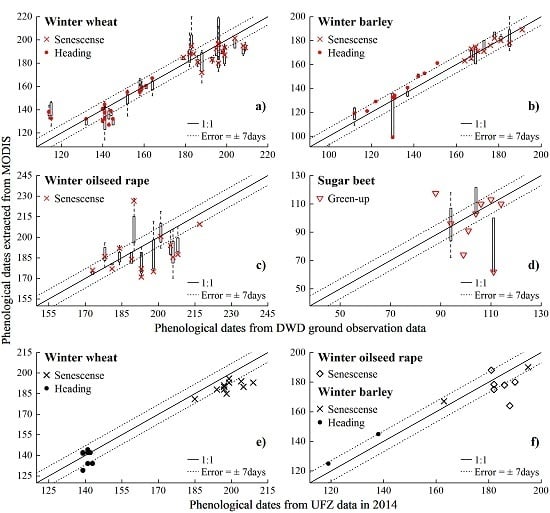
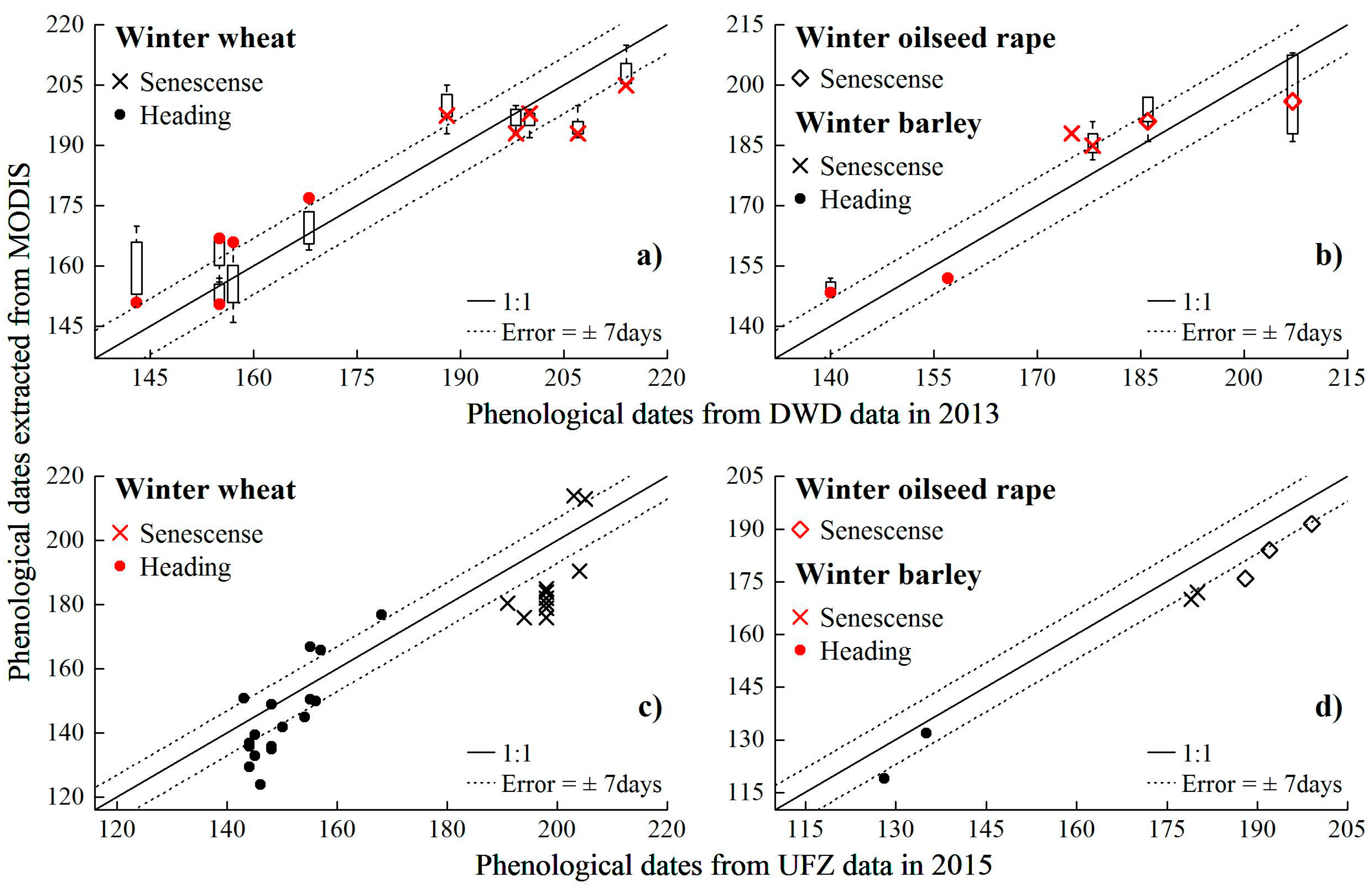
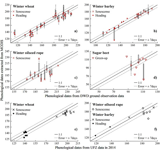
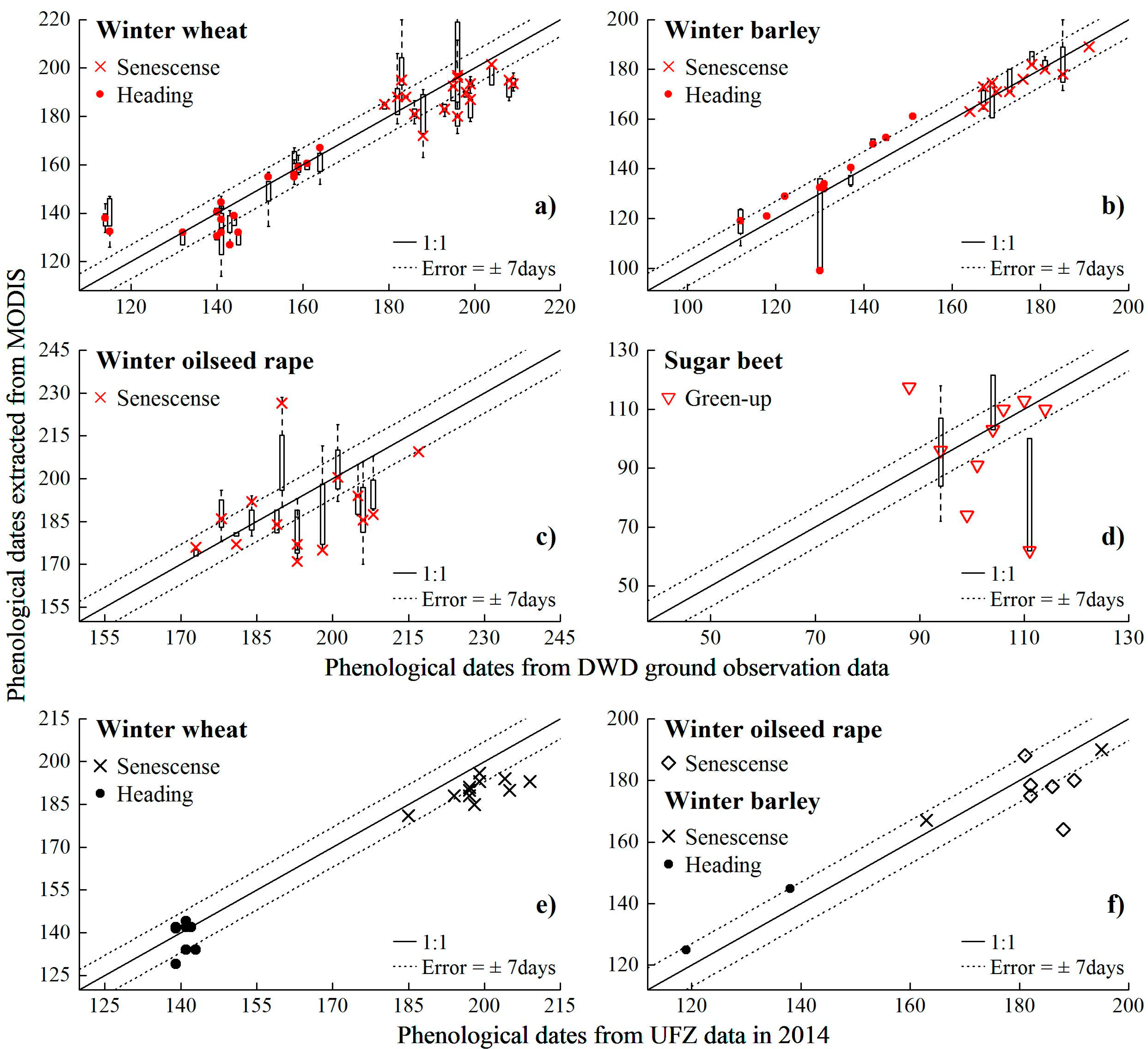
3.3. Validation Results Using the Savitzky–Golay Filter

The comparisons between MODIS phenometrics and field data in 2013 and 2015 yielded more diverse RMSE than the four-year calibration results (Table 4). There was a very good agreement between satellite-derived green-up dates and field observations for winter barley (RMSE = 6.17 days) and for oilseed rape (RMSE = 5.1 days), but these results were based on only two validation samples. Almost all MODIS senescence dates of winter-crop fields were evidently earlier than UFZ observations (Figure 6a,b). For these fields, the local minimum NDVI values close to harvest were not selected by BISE, because NDVI values continued increasing in a short period of time. Satellite-derived heading dates of winter barley were also earlier than in our UFZ data, but those of winter wheat showed no clear pattern of under- or over-estimation. The green-up of sugar beet showed a RMSE of two weeks with a limited sample size.
Similar to the calibration results, extracted phenological dates of closest fields did not always have the best agreement with DWD data (Figure 6c,d). Generally, near each DWD station with available phenological data in 2013, the variance of phenometrics was relatively small and there were also no extremely large outliers.

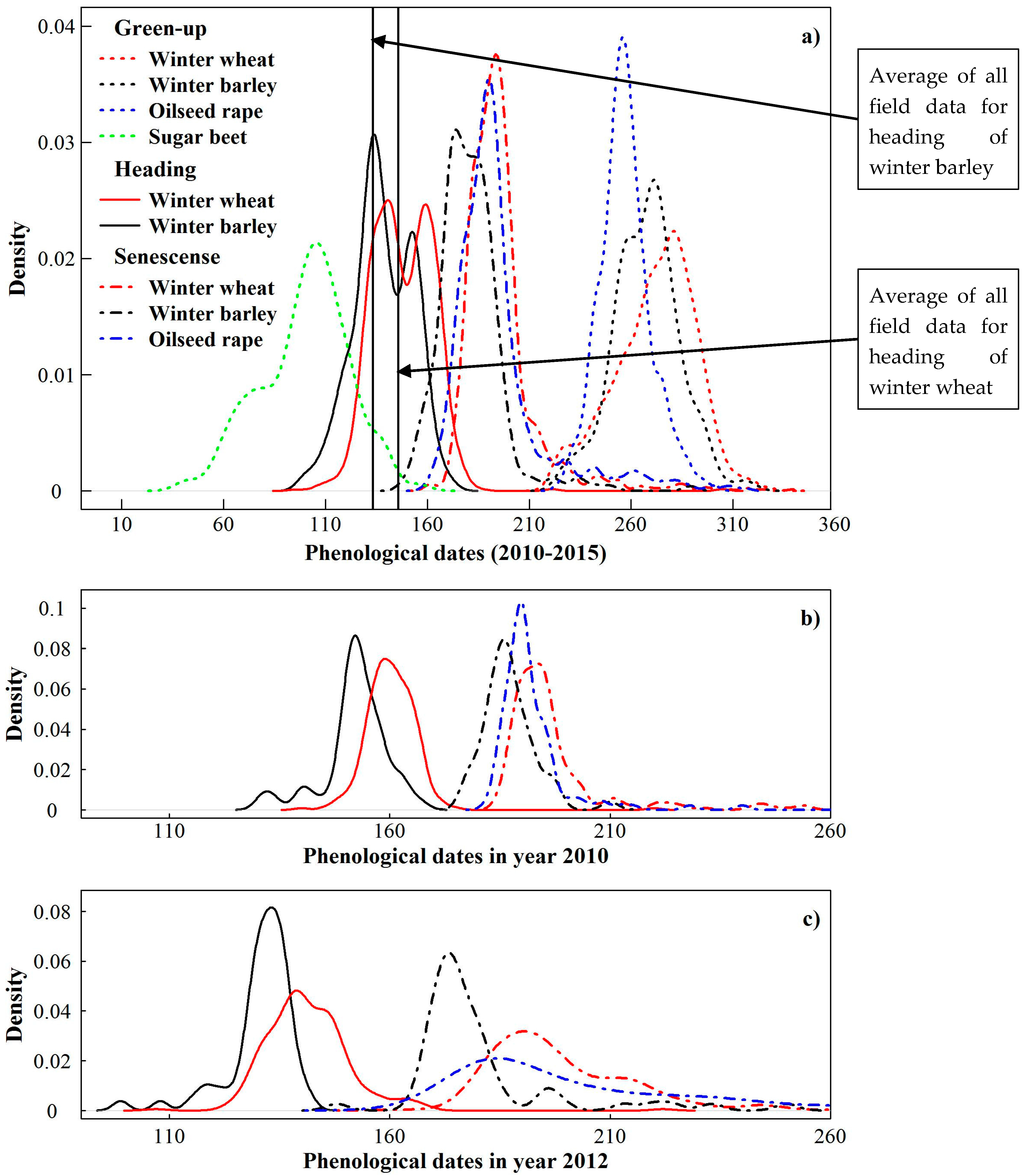
3.4. Phenometrics at Regional Scale

Phenological dates of major crops were calculated using median values of homogeneous MODIS pixels within all fields in our study area and are presented in Figure 7a. The double-peak features on the top of each density curve were mainly the results of inter-annual variation. In 2010 and 2013, satellite-derived heading and senescence dates were significantly later than those in other years. The density plots in Figure 7b,c enable the comparison between one earlier year (2010) and one later year (2012). Although outliers were noticeable especially from senescence stages, only 5.2% of the extracted senescence dates were later than 230 Julian day.
Heading and ripeness stages of winter barley were found to occur earlier than the other two winter crops (Figure 7a). The averages of all field observations (DWD and UFZ) for heading and ripeness of winter barley were 133.3 and 175.9 Julian day, respectively. For winter wheat and oilseed rape those averages amounted to 145.8 and 195.2 Julian day. Moreover, the average emergence dates based on all field data were 247.5, 271.3 and 283.8 Julian day for oilseed rape, winter barley and winter wheat, respectively. Overall, phenometrics at the regional scale matched the crop calendar and the regional in situ observations.
The green-up dates of all four major crops within fields with homogeneous MODIS pixels in this region showed the largest mean standard deviation of 12.5 days, followed by the senescence dates (mean standard deviation 7.1 days). The smallest variance occurred in heading of winter cereals (average standard deviation: 5 days). The within-field variability was to some extent affected by the uncertainty of phenometrics calculation, especially for the green-up, which showed relatively high RMSE values on the whole.

4. Discussion

4.1. Noise Reduction of NDVI Time Series

The BISE algorithm was used to construct MODIS NDVI curves from daily remote sensing data for agricultural applications [35,36]. The algorithm with adjusted sliding period minimised the risk of selecting noisy NDVI data, and retained more valuable observations at the same time. We found that the calibration results were not very sensitive to the sliding period (∆RMSE = 1.56 days for sliding periods in the range of 20–35 days), which reduces the complexity of BISE for similar applications. Nevertheless, we suggest that the algorithm needs to be re-adjusted/calibrated for areas with relatively extreme climate conditions, such as tropical regions. Although snow/cloud masks were applied and bare soil background (NDVI < 0.1) was removed, many noisy NDVI values remained in the winter season. In some cases, these values were selected by BISE because of limited noiseless data within one sliding period. This resulted in deep depressions in the NDVI curve which in turn affected the derived phenometrics (decreased regional minimum NDVI values).
Among the four algorithms tested, SG performed best when evaluated on the basis of RMSE between MODIS-estimated and ground-based phenostages. SG has the ability to smooth unevenly spaced BISE-corrected time-series [12] and the second-order polynomials preserved the subtle information related to crop phenology. Besides, SG indicated its ability to compensate situations when inter-annual vegetation variations are complicated, e.g., when a winter crop is followed by a summer crop. However, the method still introduces some bias for the part of the data that has large gaps, particularly in winter. Model fitting should be tested in the future when only one species or one phenostage is studied.

4.2. Validation with Ground Observations

The comparison of satellite-based phenometrics with more than 200 ground observations was conducted for four different crops over 6 years. Each observation was made when about 50% of the plants in the observed field had reached the corresponding stage. Such representative data obtained according to this criterion can be used for comparison with homogeneous 250-m MODIS pixels. Mixed pixel situations which may blur the accuracy of the analysis could be avoided by the inclusion of crop maps. However, some uncertainty in the field data could not be eliminated. For instance, the exact locations of the observed fields near each DWD station were undocumented. With the support of the crop map, however, we could at least assure that the field actually recorded by the DWD observer was included. Moreover, intra-field heterogeneity of crop growth likely introduced additional uncertainty. The phenometrics standard deviation of fields which contained at least one homogeneous MODIS pixel within a 3-km radius of each DWD station varied 1–4 weeks, mainly influenced by the differences of agricultural management. It is also very difficult to assess and determine one DWD/BBCH stage for large fields > 10 ha as it occurred in the study region, especially during the senescence, when observed data could be very subjective and representative for a small part of the observation site only. More detailed within-field sampling of phenology would require many experienced observers.
Although UFZ records were adjusted according to the DWD standard (around 2 days), there might still be remaining uncertainty, assuming that the correct BBCH codes were recorded by our team on a weekly basis. From Figure 2, it is clear that the rate of phenological development within different phases of different crops varied distinctly. In future studies, we suggest that the observers should be aware of the general crop calendar of the region and then adjust the sampling-time interval according to targeted phenostages of the species.

4.3. Phenometrics Extraction

The performance of the four optimised local thresholds varied between species and growth stages. Several constraints were applied on the smoothed NDVI time series to reduce outliers of phenometrics. A similar strategy was used in other studies on phenology monitoring for different crops [20,24]. The senescence dates calculated with a local threshold of 0.41 had a very close link to the DWD ripeness stage (RMSE within 1–2 weeks). During crop ripening, the weather is usually in favourable conditions. The decline of NDVI values was also very pronounced, which explained why the ripeness stage of winter crops was not very sensitive to slight adjustments of the local threshold (increase or decrease of the local threshold by 0.01–0.02). Furthermore, the thresholds of senescence stage optimised using different algorithms (SG, FFT, linear interpolation) were found in a very narrow range (Table 2). This was also observed from other stages, which was probably related to leaf area index and leaf angle.
Although the estimation of emergence stage of winter and summer crops was challenging, our phenometrics differed significantly from the general onset of greening using low thresholds of less than 0.3. For winter crops, such large differences in the threshold (compared to standard local threshold of 0.5) led to improvement of the emergence stage by 8.89 days. Even though other studies have also used similar thresholds for estimating the emergence stage of crops in VI curves [25,26,37], our analysis was based on the knowledge of field boundaries and the corresponding crop types. The relatively high RMSE had two main causes. Firstly, it was strongly affected by poor quality of satellite data (low viewing angle, heavy cloud, snow effect, etc.) at the beginning and the end of the year. Secondly, with suitable temperature and rainfall in August and September, new leaves grew from some of the grains which remained in the soil after harvest. This resulted in a strong green signal, which can shift the predicted green-up dates of winter crops of the following year towards earlier values and also, to some extent, influence the satellite-derived senescence dates (Figure 7a). Zhao et al. [20] speculated that the low accuracy of green-up estimation was probably also due to the soil background. An accurate estimation for winter wheat emergence (RMSE = 3.2 days) was obtained using geostationary satellite data (1-km spatial resolution) in northern India [22]. However, this result was extracted with semi-homogeneous validation pixels of which only less than 15% had more than 90% wheat fraction.
The date with maximum NDVI compared to field heading stage of winter cereals had a RMSE of around one week, without any consistent pattern of temporal offsets, except for winter wheat in 2015. Because (late) booting stage is slightly earlier (around 5 days) than the beginning of heading (BBCH 51/DWD 18), the relationship between dates corresponding to the maximum NDVI and heading stage should be further investigated. Wang et al. [38] found that earlier onset of heading was estimated using NDVI rather than EVI2 (Two-band Enhanced Vegetation Index) [39] for rice, thus our results could be improved by using alternative VIs, e.g., the Wide Dynamic Range Vegetation Index [40] and EVI2, to reduce NDVI saturation effects and improve heading stage estimation. Two DWD wheat heading records in 2011 and 2012 deviated considerably from MODIS-derived dates of fields near the Meisdorf station, which is very unusual in contrast to the phenological records in other years. Despite prior checking, a filtering procedure such as proposed by Siebert and Ewert [27] is suggested for future work.

5. Conclusions

In this study, we extracted MODIS phenometrics of major crops in central Germany from 2010 to 2015. For the first time, extensive field-observed data over six cropping seasons was used to calibrate and validate phenometrics of winter wheat, winter barley, oilseed rape, and sugar beet. Such a considerable amount of ground-truth data enabled us to investigate the relationship between satellite-derived and field-observed phenostages reliably. As phenometrics were more sensitive to different settings of the smoothing algorithms and thresholds than the sliding period, our results proved that BISE can be easily applied for phenology monitoring over large areas with similar climate conditions.
Comparatively low RMSE values for four crops suggest that BISE in combination with SG can be beneficial for monitoring different phenostages, especially winter crops. Our satellite-derived phenometrics, which represent specific agronomic stages, can assist yield estimation, crop management and crop identification over large areas. The optimised thresholds of winter crops were independent of our targeted species. The date calculated using a local threshold of 0.41 during the senescence period was closely related to the ripeness stage, with RMSE from 3.8 to 15.24 days. The estimated heading stage using maximum NDVI had an RMSE of 6.84–10.48 days compared to field data. With the local threshold of 0.1, the green-up stage of winter crops was improved by more than one week. Future research should focus on an improved assessment by prior checking of the field data. In addition, maize can also be investigated in the future to increase the applicability of this method.
MODIS-derived phenometrics showed various intra- and inter-field differences of each phenostage which were also observed in our field trips. This highlights the need of recording the exact locations of observed fields in the DWD database. Such geospatial information not only can advance remote sensing-related phenology research, but also benefit a wide range of applications, such as yield estimation and crop modelling. With the arrival of Sentinel-2 data from 2016, there is a great potential to use additional indices of even higher spatial resolution for monitoring crop phenology.

Acknowledgments

This work was supported by PhenoS project (grant number 50EE1262), and funded by the German Federal Ministry for Economic Affairs and Energy. We would like to acknowledge those who contributed to collect field phenology data: Gundula Schulz, Steffen Lehmann, Gudrun Schuhmann and Steffi Erfurth. We also thank the Ministry of Agriculture and Environment of Saxony-Anhalt for providing the crop maps, as well as Maximilian Lange for providing the ‘phenex’ R package and related scripts.

Author Contributions

Xingmei Xu, Christopher Conrad and Daniel Doktor all conceived and designed the experiments; Xingmei Xu performed the experiments and analysed the data; Daniel Doktor contributed materials and analysis tools; Xingmei Xu wrote the paper.

Conflicts of Interest

The authors declare no conflict of interest. The founding sponsors had no role in the design of the study; in the collection, analyses, or interpretation of data; in the writing of the manuscript, and in the decision to publish the results.

References

  1. Moran, M.S.; Inoue, Y.; Barnes, E.M. Opportunities and limitations for image-based remote sensing in precision crop management. Remote Sens. Environ. 1997, 61, 319–346. [Google Scholar] [CrossRef]
  2. Thenkabail, P.S. Global croplands and their importance for water and food security in the twenty-first century: Towards an ever green revolution that combines a second green revolution with a blue revolution. Remote Sens. 2010, 2, 2305–2312. [Google Scholar] [CrossRef]
  3. Fischer, A. A model for the seasonal-variations of vegetation indexes in coarse resolution data and its inversion to extract crop parameters. Remote Sens. Environ. 1994, 48, 220–230. [Google Scholar] [CrossRef]
  4. Marinho, E.; Vancutsem, C.; Fasbender, D.; Kayitakire, F.; Pini, G.; Pekel, J.-F. From Remotely Sensed Vegetation Onset to Sowing Dates: Aggregating Pixel-Level Detections into Village-Level Sowing Probabilities. Remote Sens. 2014, 6, 10947–10965. [Google Scholar] [CrossRef]
  5. Simms, D.M.; Waine, T.W.; Taylor, J.C.; Juniper, G.R. The application of time-series MODIS NDVI profiles for the acquisition of crop information across Afghanistan. Int. J. Remote Sens. 2014, 35, 37–41. [Google Scholar] [CrossRef]
  6. Sehgal, V.K.; Jain, S.; Aggarwal, P.K.; Jha, S. Deriving Crop Phenology Metrics and Their Trends Using Times Series NOAA-AVHRR NDVI Data. J. Indian Soc. Remote Sens. 2011, 39, 373–381. [Google Scholar] [CrossRef]
  7. Wardlow, B.D.; Kastens, J.H.; Egbert, S.L. Using USDA crop progress data for the evaluation of greenup onset date calculated from MODIS 250-meter data. Photogramm. Eng. Remote Sens. 2006, 72, 1225–1234. [Google Scholar] [CrossRef]
  8. Myneni, R.B.; Hall, F.G.; Sellers, P.J.; Marshak, A.L. Interpretation of spectral vegetation indexes. IEEE Trans. Geosci. Remote Sens. 1995, 33, 481–486. [Google Scholar] [CrossRef]
  9. Bauer, M.E. Spectral Inputs to Crop Identification and Condition Assessment. Proc. IEEE 1985, 73, 1071–1085. [Google Scholar] [CrossRef]
  10. Sakamoto, T.; Yokozawa, M.; Toritani, H.; Shibayama, M.; Ishitsuka, N.; Ohno, H. A crop phenology detection method using time-series MODIS data. Remote Sens. Environ. 2005, 96, 366–374. [Google Scholar] [CrossRef]
  11. Domínguez, J.A.; Kumhálová, J.; Novák, P. Winter oilseed rape and winter wheat growth prediction using remote sensing methods. Plant Soil Environ. 2015, 61, 410–416. [Google Scholar]
  12. Pan, Z.; Huang, J.; Zhou, Q.; Wang, L.; Cheng, Y.; Zhang, H.; Blackburn, G.A.; Yan, J.; Liu, J. Mapping crop phenology using NDVI time-series derived from HJ-1 A/B data. Int. J. Appl. Earth Obs. Geoinf. 2015, 34, 188–197. [Google Scholar] [CrossRef]
  13. Herbek, J.; Lee, C. A Comprehensive Guide to Wheat Management in Kentucky; University of Kentucky College of Agriculture: Lexington, KY, USA, 2009. [Google Scholar]
  14. Holben, B.N. Characteristics of maximum-value composite images from temporal AVHRR data. Int. J. Remote Sens. 1986, 7, 1417–1434. [Google Scholar] [CrossRef]
  15. Viovy, N.; Arino, O.; Belward, A. S. The Best Index Slope Extraction (BISE): A method for reducing noise in NDVI time-series. Int. J. Remote Sens. 1992, 13, 1585–1590. [Google Scholar] [CrossRef]
  16. Chen, J.; Jönsson, P.; Tamura, M.; Gu, Z.; Matsushita, B.; Eklundh, L. A simple method for reconstructing a high-quality NDVI time-series data set based on the Savitzky-Golay filter. Remote Sens. Environ. 2004, 91, 332–344. [Google Scholar] [CrossRef]
  17. Savitzky, A.; Golay, M.J.E. Smoothing and Differentiation of Data by Simplified Least Squares Procedures. Anal. Chem. 1964, 36, 1627–1639. [Google Scholar] [CrossRef]
  18. Zhu, W.; Pan, Y.; He, H.; Wang, L.; Mou, M.; Liu, J. A changing-weight filter method for reconstructing a high-quality NDVI time series to preserve the integrity of vegetation phenology. IEEE Trans. Geosci. Remote Sens. 2012, 50, 1085–1094. [Google Scholar] [CrossRef]
  19. De Beurs, K.M.; Henebry, G.M. Spatio-temporal statistical methods for modelling land surface phenology. In Phenological Research: Methods for Environmental and Climate Change Analysis; Springer: Berlin/Heidelberg, Germany, 2010; pp. 177–208. [Google Scholar]
  20. Zhao, H.; Yang, Z.; Di, L.; Li, L.; Zhu, H. Crop phenology date estimation based on NDVI derived from the reconstructed MODIS daily surface reflectance data. In Proceedings of the 2009 17th International Conference on Geoinformatics, Fairfax, VA, USA, 12–14 August 2009; pp. 1–6.
  21. Zhang, X.; Friedl, M.A.; Schaaf, C.B.; Strahler, A.H.; Hodges, J.C.F.; Gao, F.; Reed, B.C.; Huete, A. Monitoring vegetation phenology using MODIS. Remote Sens. Environ. 2003, 84, 471–475. [Google Scholar] [CrossRef]
  22. Vyas, S.; Nigam, R.; Patel, N.K.; Panigrahy, S. Extracting Regional Pattern of Wheat Sowing Dates Using Multispectral and High Temporal Observations from Indian Geostationary Satellite. J. Indian Soc. Remote Sens. 2013, 41, 855–864. [Google Scholar] [CrossRef]
  23. Yang, H.; Li, Z.; Chen, E.; Zhao, C.; Yang, G.; Casa, R.; Pignatti, S.; Feng, Q. Temporal polarimetric behavior of oilseed rape (Brassica napus L.) at c-band for early season sowing date monitoring. Remote Sens. 2014, 6, 10375–10394. [Google Scholar] [CrossRef]
  24. Zhang, Z.; Song, X.; Chen, Y.; Wang, P.; Wei, X.; Tao, F. Dynamic variability of the heading–flowering stages of single rice in China based on field observations and NDVI estimations. Int. J. Biometeorol. 2015, 59, 643–655. [Google Scholar] [CrossRef] [PubMed]
  25. Sakamoto, T.; Wardlow, B.D.; Gitelson, A.A.; Verma, S.B.; Suyker, A.E.; Arkebauer, T.J. A Two-Step Filtering approach for detecting maize and soybean phenology with time-series MODIS data. Remote Sens. Environ. 2010, 114, 2146–2159. [Google Scholar] [CrossRef]
  26. Zeng, L.; Wardlow, B.D.; Wang, R.; Shan, J.; Tadesse, T.; Hayes, M.J.; Li, D. A hybrid approach for detecting corn and soybean phenology with time-series MODIS data. Remote Sens. Environ. 2016, 181, 237–250. [Google Scholar] [CrossRef]
  27. Siebert, S.; Ewert, F. Spatio-temporal patterns of phenological development in Germany in relation to temperature and day length. Agric. For. Meteorol. 2012, 152, 44–57. [Google Scholar] [CrossRef]
  28. Rouse, J.W.; Hass, R.H.; Schell, J.A.; Deering, D.W. Monitoring vegetation systems in the great plains with ERTS. Third Earth Resour. Technol. Satell. Symp. 1973, 1, 309–317. [Google Scholar]
  29. Geng, L.; Ma, M.; Yu, W.; Wang, X.; Jia, S. Validation of the MODIS NDVI products in different land-use types using in situ measurements in the heihe river basin. IEEE Geosci. Remote Sens. Lett. 2014, 11, 1649–1653. [Google Scholar] [CrossRef]
  30. Hall, D.K.; Riggs, G.A. Accuracy assessment of the MODIS snow products. Hydrol. Process. 2007, 21, 1534–1547. [Google Scholar] [CrossRef]
  31. Deutscher Wetterdienst Aktueller Stand der Phänologie in Deutschland. Available online: ftp://ftp-cdc.dwd.de/pub/CDC/observations_germany/phenology/annual_reporters/crops/recent/ (accessed on 9 January 2015).
  32. Meier, U.; Bleiholder, H.; Buhr, L.; Feller, C.; Hack, H.; Heß, M.; Lancashire, P.; Schnock, U.; Stauß, R.; van den Boom, T.; et al. The BBCH system to coding the phenological growth stages of plants-history and publications. J. Kulturpflanzen 2009, 61, 41–52. [Google Scholar]
  33. Lange, M.; Doktor, D. R-Package “phenex”—Auxiliary Functions for Phenological Data Analysis. Available online: http://cran.r-project.org/web/packages/phenex/ (accessed on 8 June 2014).
  34. Press, W.H.; Teukolsky, S.A.; Vetterling, W.T.; Flannery, B.P. Numerical Recipes in C: The Art of Scientific Computing, 2nd ed.; Cambridge University Press: Cambridge, UK, 1992. [Google Scholar]
  35. Di, L.; Yu, E.G.; Yang, Z.; Shrestha, R.; Kang, L.; Zhang, B.; Sw, I.A. Remote sensing based crop growth stage estimation model. In Proceedings of the 2015 IEEE International Geoscience and Remote Sensing Symposium (IGARSS), Milan, Italy, 26–31 July 2015; pp. 2739–2742.
  36. Kotsuki, S.; Tanaka, K. SACRA-a method for the estimation of global high-resolution crop calendars from a satellite-sensed NDVI. Hydrol. Earth Syst. Sci. 2015, 19, 4441–4461. [Google Scholar] [CrossRef]
  37. Lobell, D.B.; Ortiz-Monasterio, J.I.; Sibley, A.M.; Sohu, V.S. Satellite detection of earlier wheat sowing in India and implications for yield trends. Agric. Syst. 2013, 115, 137–143. [Google Scholar] [CrossRef]
  38. Wang, J.; Huang, J.; Wang, X.; Jin, M.; Zhou, Z.; Guo, Q.; Zhao, Z.; Huang, W.; Zhang, Y.; Song, X. Estimation of rice phenology date using integrated HJ-1 CCD and Landsat-8 OLI vegetation indices time-series images. J. Zhejiang Univ. Sci. B 2015, 16, 832–844. [Google Scholar] [PubMed]
  39. Jiang, Z.; Huete, A.R.; Kim, Y.; Didan, K. 2-band Enhanced Vegetation Index without a blue band and its application to AVHRR data. In Remote Sensing and Modeling of Ecosystems for Sustainability IV; SPIE: Bellingham, WA, USA, 2007; Volume 6679, p. 667905. [Google Scholar]
  40. Gitelson, A.A. Wide Dynamic Range Vegetation Index for remote quantification of biophysical characteristics of vegetation. J. Plant Physiol. 2004, 161, 165–173. [Google Scholar] [CrossRef] [PubMed]
Figure 1. Overview of the study area in central Germany. The green box in the auxiliary map indicates Moderate Resolution Imaging Spectrometer (MODIS) data coverage in our study. The large green area in the satellite image is part of the Harz Mountains. Yellow labels represent the names of towns including those where German Meteorological Service (DWD) stations are located. Satellite imagery was available as basemap in Esri’s World Imagery map.
Remotesensing 09 00254 g001
Figure 2. BBCH stages for four crop species from our own field measurements (hereafter referred to as UFZ data) in 2015.
Remotesensing 09 00254 g002
Figure 3. Example of a MODIS Normalized Difference Vegetation Index (NDVI) time-series for winter wheat. MODIS NDVI values of less than 0.1 were removed after applying snow and cloud mask. Only selected NDVI values by Best Index Slope Extraction (BISE; red dots with crosses) were used to construct 3-year NDVI profile for phenometrics extraction. The blue curve is an example of using the Savitzky–Golay filter (SG) algorithm for smooth interpolation.
Remotesensing 09 00254 g003
Figure 4. Processing chain (RMSE: root mean square error).
Remotesensing 09 00254 g004
Figure 5. Calibration results of satellite-derived phenological dates for different crops in: (ad) 2010, 2011, 2012 and 2014 versus DWD data; (e,f) 2014 versus UFZ data. Red-coloured symbols indicate fields which were closest to DWD stations. Each box represents phenostages of all fields which were within 3 km around one DWD station.
Remotesensing 09 00254 g005
Figure 6. Validated satellite-derived phenological dates for different crops in: (a,b) 2013 versus DWD data; (c,d) 2015 versus UFZ data. Red-coloured symbols indicate fields which were closest to DWD stations. Each box represents phenostages of all fields which were within 3 km around one DWD station.
Remotesensing 09 00254 g006
Figure 7. Density of different phenometrics calculated using fields with homogeneous MODIS pixels: (a) from 2010 to 2015, (b) from 2010 and (c) from 2012. The averages of all field data for heading of winter wheat (133.3) and winter barley (145.8) are also shown.
Remotesensing 09 00254 g007
Table 1. Targeted phenostages of different major crops in this study based on DWD and Biologische Bundesanstalt für Land- und Forstwirtschaft, Bundessortenamt und CHemische Industrie (BBCH) scale [32].
CropDWD Stage IDDWD StageBBCHStage Description
Winter wheat/barley12emergence10The first leaf emerges from the coleoptile and the rows of plants are already visible
18heading51Tip of inflorescence emerged from sheath, first spikelet just visible
21yellow ripeness−87 1The first grains have finished changing their colour from green to yellow and can be removed easily from the ear. The individual grains can be broken over the thumbnail, and the contents of the grains are plastic to hard.
Oilseed rape12emergence10The plants have broken through the surface of the soil and have reached a height of approximately 1 cm
22full ripeness−87 1Most of the rape grains are black on one side
Sugar beet12emergence10First leaf visible: cotyledons horizontally unfolded
1 Agreement to a large extent; phase can occur slightly earlier than corresponding BBCH micro stage.
Table 2. Calibrated sliding period and thresholds for four methods with field data in 2010, 2011, 2012 and 2014. RMSE in days was calculated with all phenostages of all four crops. d and m represent the degree of polynomial fitting and the middle width of the moving window, respectively. s is the smoothing intensity of fast Fourier transform (FFT).
MethodMethod SettingsSliding Period (Days)PhenometricsLocal ThresholdRMSE
Winter CropsSugar Beet(Days)
SGd = 2; m = 521green-up0.100.2912.76
senescence0.41
Linear 23green-up0.170.3013.76
senescence0.5
FFTs = 128green-up0.120.2613.96
senescence0.48
Spline 31 15.91
Table 3. RMSE in days between the green-up, heading, and senescence dates calculated using homogeneous MODIS pixels and field data (DWD and UFZ) for different crops. The corresponding number of field observations for calibration is given in brackets.
RMSE (Days)YearGreen-UpHeadingSenescence
Winter wheat2010–2012, 201417.61(14)8.52(25)9.43(29)
Winter barley2010–2012, 201415.67(10)10.38(13)3.80(13)
Oilseed rape2010–2012, 201413.20(17) 15.24(20)
Sugar beet2010–2012, 201421.19(9)
Table 4. RMSE in days between senescence, heading and green-up dates calculated using homogeneous MODIS pixels and field data (DWD and UFZ) for different crops in 2013 and 2015. The corresponding number of field observations for validation is given in brackets.
RMSE (Days)YearGreen-UpHeadingSenescence
Winter wheat2013, 201520.37(6)10.48(17)13.59(17)
Winter barley2013, 20156.17(2)6.84(4)9.53(4)
Oilseed rape2013, 20155.10(2) 9.06(5)
Sugar beet2013, 201514.17(4)

