
Retrieval of Chlorophyll-a and Total Suspended Solids Using Iterative Stepwise Elimination Partial Least Squares (ISE-PLS) Regression Based on Field Hyperspectral Measurements in Irrigation Ponds in Higashihiroshima, Japan


Abstract
:
1. Introduction
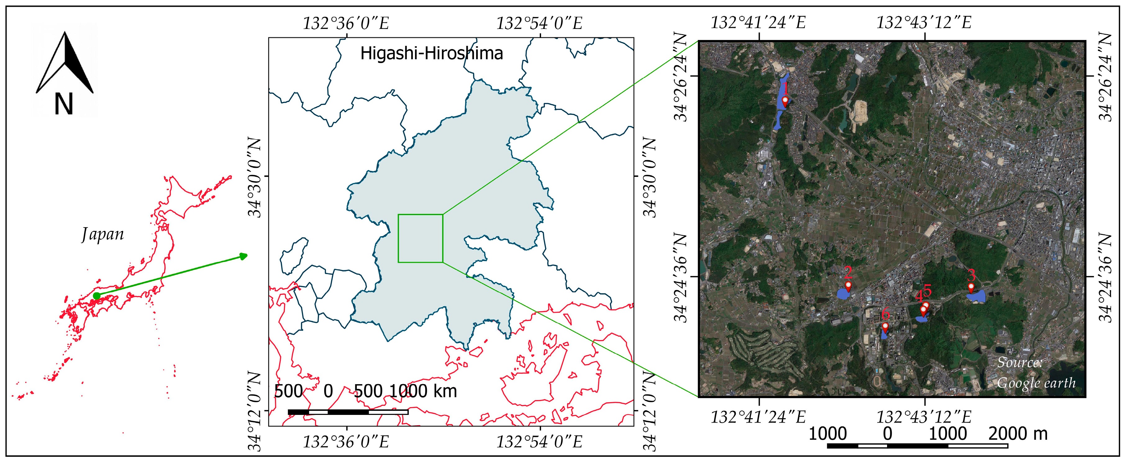
2. Study Area
3. Materials and Methods
3.1. Measurement of Water Surface Reflectance
3.2. Water Sampling and Chemical Analysis
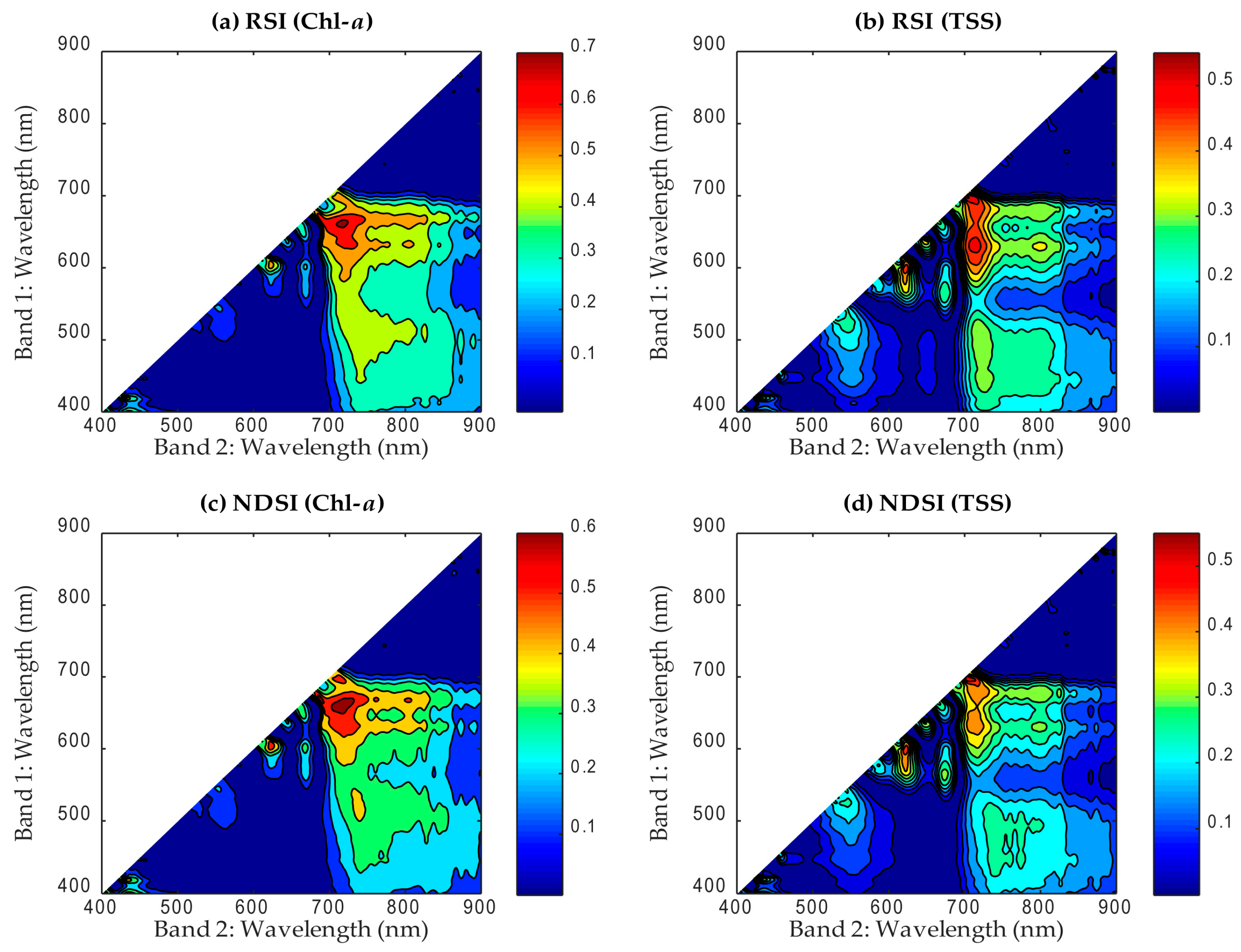
3.3. Ratio Spectral Index and Normalized Difference Spectral Indices
3.4. Full Spectrum Partial Least Squares Regression
3.5. Iterative Stepwise Elimination Partial Least Squares Regression
3.6. Evaluation of Predictive Ability
4. Results
4.1. Chl-a and TSS Concentrations in Irrigation Ponds
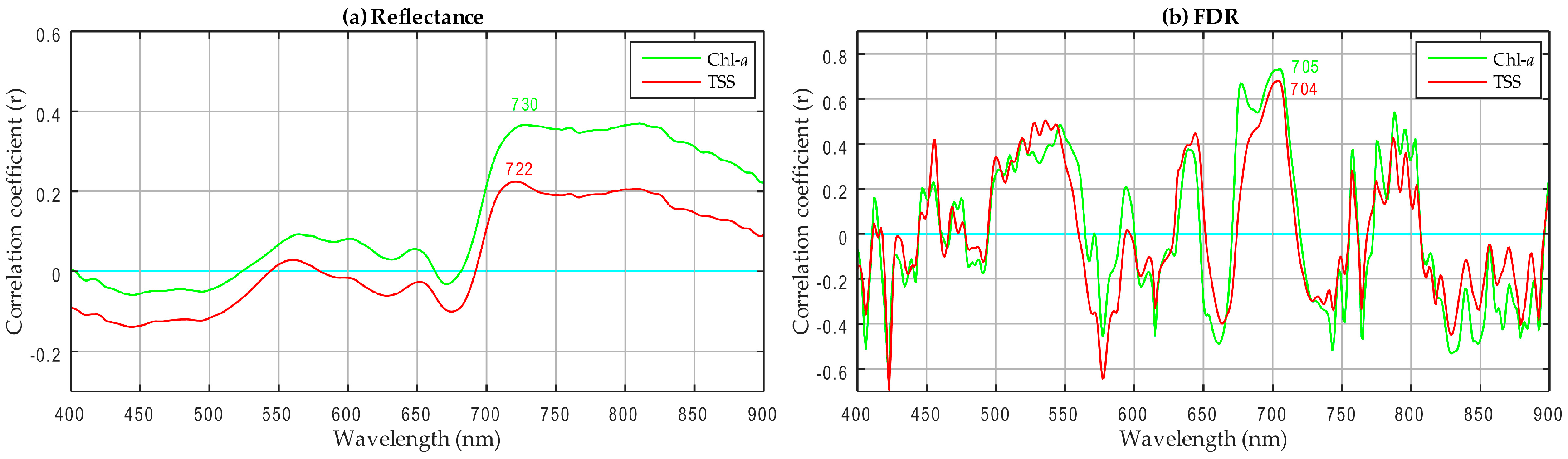
4.2. Comparison of Simple Linear Regression Models
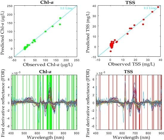
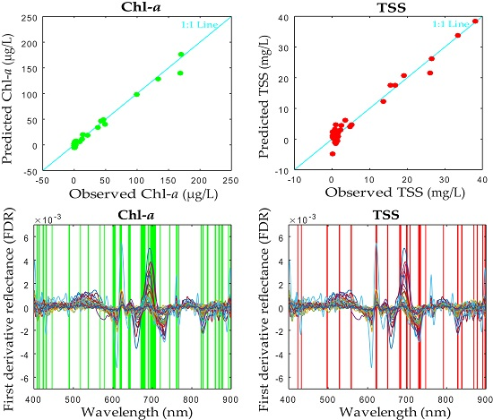
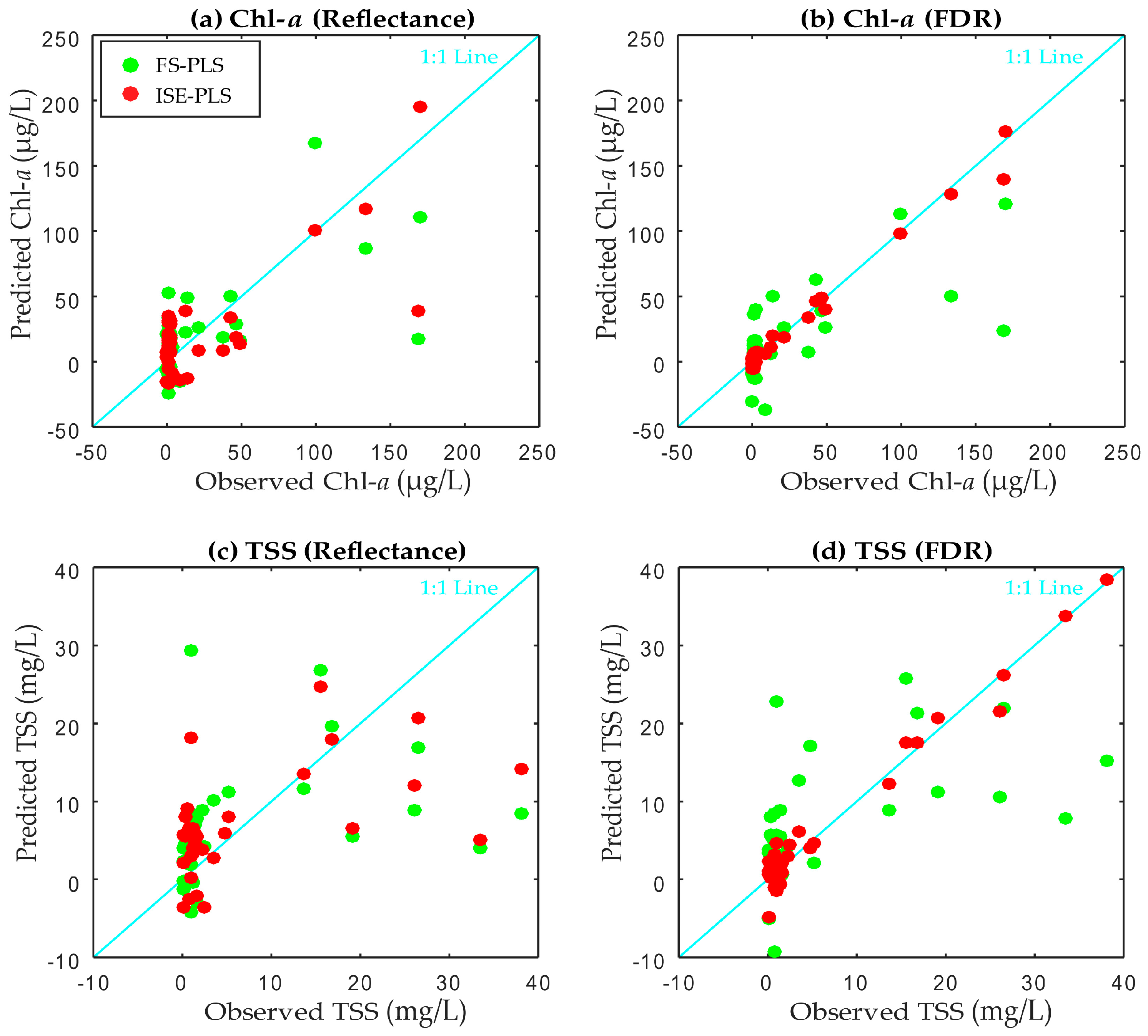
4.3. FS–PLS and ISE–PLS Models
5. Discussion
5.1. Evaluation of the Predictive Abilities of Simple Linear Regression Models
5.2. Evaluation of the Predictive Abilities of FS–PLS and ISE–PLS
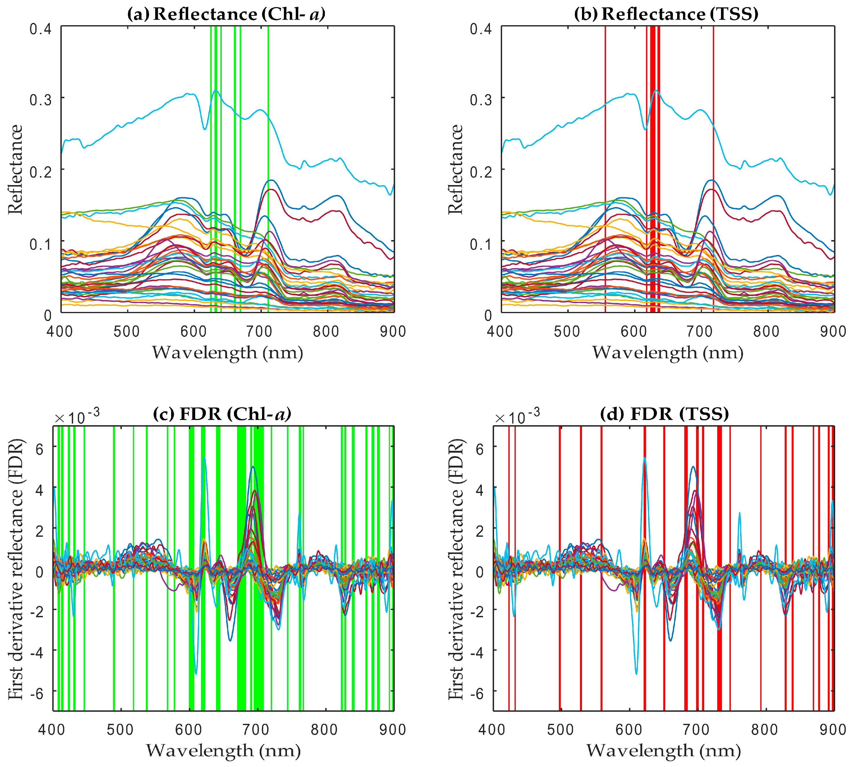
5.3. Importance of Selected Wavebands in ISE–PLS
6. Conclusions
Acknowledgments
Author Contributions
Conflicts of Interest
References
- Mateo-Sagasta, J.; Burke, J. SOLAW Background Thematic Report—TR08; FAO: Rome, Italy, 2010. [Google Scholar]
- Yang, X.E.; Wu, X.; Hao, H.L.; He, Z.L. Mechanisms and assessment of water eutrophication. J. Zhejiang Univ. Sci. B 2008, 9, 197–209. [Google Scholar] [CrossRef] [PubMed]
- Rönnberg, C.; Bonsdorff, E. Baltic Sea eutrophication: Area-specific ecological consequences. Hydrobiologia 2004, 514, 227–241. [Google Scholar] [CrossRef]
- World Health Organization (WHO). Guidelines for Drinking-Water Quality, 4th ed.; WHO: Geneva, Switzerland, 2011. [Google Scholar]
- Latif, Z.; Tasneem, M.A.; Javed, T.; Butt, S.; Fazil, M.; Ali, M.; Sajjad, M.I. Evaluation of Water-Quality by Chlorophyll and Dissolved Oxygen. Water Resour. South Present Scenar. Future Prospect. 2003, 7, 123–135. [Google Scholar]
- Lu, F.; Chen, Z.; Liu, W.; Shao, H. Modeling chlorophyll-a concentrations using an artificial neural network for precisely eco-restoring lake basin. Ecol. Eng. 2016, 95, 422–429. [Google Scholar] [CrossRef]
- Sikorska, A.E.; Del Giudice, D.; Banasik, K.; Rieckermann, J. The value of streamflow data in improving TSS predictions—Bayesian multi-objective calibration. J. Hydrol. 2015, 530, 241–254. [Google Scholar] [CrossRef]
- Fondriest Environmental, Inc. Turbidity, Total Suspended Solids and Water Clarity; Fundamentals of Environmental Measurements, 2014. Available online: http://www.fondriest.com/environmental-measurements/parameters/water-quality/turbidity-total-suspended-solids-water-clarity (accessed on 3 November 2016).
- Bash, J. Effects of Turbidity and Suspended Solids on Salmonids; Center for Streamside Studies, University of Washington: Seattle, WA, USA, 2001; p. 74. [Google Scholar]
- Davies-Colley, R.J.; Smith, D.G. Turbidity, suspended sediment, and water clarity: A review. J. Am. Water Resour. Assoc. 2001, 37, 1085–1101. [Google Scholar] [CrossRef]
- Shafique, N.A.; Fulk, F.; Autrey, B.C.; Flotemersch, J. Hyperspectral Remote Sensing of Water Quality Parameters for Large Rivers in the Ohio River Basin. In Proceedings of the First Interagency Conference on Research in the Watersheds, USDA Agricultural Research Service, Washington, DC, USA, 27–30 October 2003.
- Voutilainen, A.; Pyhälahti, T.; Kallio, K.Y.; Pulliainen, J.; Haario, H.; Kaipio, J.P. A filtering approach for estimating lake water quality from remote sensing data. Int. J. Appl. Earth Obs. Geoinform. 2007, 9, 50–64. [Google Scholar] [CrossRef]
- O’Reilly, J.E.; Maritorena, S.; Mitchell, B.G.; Siegel, D.A.; Carder, K.L.; Garver, S.A.; Kahru, M.; McClain, C. Ocean color chlorophyll algorithms for SeaWiFS. J. Geophys. Res. 1998, 103, 24937–24953. [Google Scholar] [CrossRef]
- Sakuno, Y.; Makio, K.; Koike, K.; Maung-Saw-Htoo-Thaw; Kitahara, S. Chlorophyll-a estimation in Tachibana bay by data Fusion of GOCI and MODIS using linear combination index algorithm. Adv. Remote Sens. 2013, 2, 292–296. [Google Scholar] [CrossRef]
- Gitelson, A.A.; Gritz, U.; Merzlyak, M.N. Relationships between leaf chlorophyll content and spectral reflectance and algorithms for nondestructive chlorophyll assessment in higher plant leaves. J. Plant Physiol. 2003, 160, 271–282. [Google Scholar] [CrossRef] [PubMed]
- Mishra, S.; Mishra, D.R. Normalized difference chlorophyll index: A novel model for remote estimation of chlorophyll-a concentration in turbid productive waters. Remote Sens. Environ. 2012, 117, 394–406. [Google Scholar] [CrossRef]
- Dall’Olmo, G.; Gitelson, A.A.; Rundquist, D.C. Towards a unified approach for remote estimation of chlorophyll-a in both terrestrial vegetation and turbid productive waters. Geophys. Res. Lett. 2003, 30, 1938. [Google Scholar] [CrossRef]
- Gitelson, A.A.; Dall’Olmo, G.; Moses, W.; Rundquist, D.C.; Barrow, T.; Fisher, T.R.; Gurlin, D.; Holz, J. A simple semi-analytical model for remote estimation of chlorophyll-a in turbid waters: Validation. Remote Sens. Environ. 2008, 112, 3582–3593. [Google Scholar] [CrossRef]
- Nechad, B.; Ruddick, K.G.; Park, Y. Calibration and validation of a generic multisensor algorithm for mapping of total suspended matter in turbid waters. Remote Sens. Environ. 2010, 114, 854–866. [Google Scholar] [CrossRef]
- Pulliainen, J.; Kallio, K.; Eloheimo, K.; Koponen, S.; Servomaa, H.; Hannonen, T.; Tauriainen, S.; Hallikainen, M. A semi-operative approach to lake water quality retrieval from remote sensing data. Sci. Total Environ. 2001, 268, 79–93. [Google Scholar] [CrossRef]
- Dall’Olmo, G.; Gitelson, A.A.; Rundquist, D.C.; Leavitt, B.; Barrow, T.; Holz, J.C. Assessing the potential of SeaWiFS and MODIS for estimating chlorophyll concentration in turbid productive waters using red and near-infrared bands. Remote Sens. Environ. 2005, 96, 176–187. [Google Scholar] [CrossRef]
- Han, L.; Rundquist, D.C. Comparison of NIR/RED ratio and first derivative of reflectance in estimating algal-chlorophyll concentration: A case study in a turbid reservoir. Remote Sens. Environ. 1997, 62, 253–261. [Google Scholar] [CrossRef]
- Inoue, Y.; Peñuelas, J.; Miyata, A.; Mano, M. Normalized difference spectral indices for estimating photosynthetic efficiency and capacity at a canopy scale derived from hyperspectral and CO2 flux measurements in rice. Remote Sens. Environ. 2008, 112, 156–172. [Google Scholar] [CrossRef]
- Stagakis, S.; Markos, N.; Sykioti, O.; Kyparissis, A. Monitoring canopy biophysical and biochemical parameters in ecosystem scale using satellite hyperspectral imagery: An application on a phlomis fruticosa Mediterranean ecosystem using multiangular CHRIS/PROBA observations. Remote Sens. Environ. 2010, 114, 977–994. [Google Scholar] [CrossRef]
- Inoue, Y.; Sakaiya, E.; Zhu, Y.; Takahashi, W. Diagnostic mapping of canopy nitrogen content in rice based on hyperspectral measurements. Remote Sens. Environ. 2012, 126, 210–221. [Google Scholar] [CrossRef]
- Wold, H. Estimation of Principal Components and Related Models by Iterative Least Squares. In Multivariate Analysis; Krishnaiaah, P.R., Ed.; Academic Press: New York, NY, USA, 1966; pp. 391–420. [Google Scholar]
- Song, K.; Li, L.; Li, S.; Tedesco, L.; Duan, H.; Li, Z.; Shi, K.; Du, J.; Zhao, Y.; Shao, T. Using partial least squares-artificial neural network for inversion of inland water Chlorophylla. IEEE Trans. Geosci. Remote Sens. 2014, 52, 1502–1517. [Google Scholar] [CrossRef]
- Ghasemi, J.; Niazi, A. Genetic-algorithm-based wavelength selection in multicomponent spectrophotometric determination by PLS: Application on copper and zinc mixture. Talanta 2003, 59, 311–317. [Google Scholar] [CrossRef]
- Kawamura, K.; Watanabe, N.; Sakanoue, S.; Inoue, Y. Estimating forage biomass and quality in a mixed sown pasture based on partial least squares regression with waveband selection. Grassl. Sci. 2008, 54, 131–145. [Google Scholar] [CrossRef]
- Swierenga, H.; Groot, P.J.; Weijer, A.P.; Derksen, M.W.J.; Buydens, L.M.C. Improvement of PLS model transferability by robust wavelength selection. Chemom. Intell. Lab. Syst. 1998, 41, 237–248. [Google Scholar] [CrossRef]
- Boggia, R.; Forina, M.; Fossa, P.; Mosti, L. Chemometric study and validation strategies in the structure-activity relationships of new class of cardiotonic agents. Quant. Struct Act. Relatsh. 1997, 16, 201–213. [Google Scholar] [CrossRef]
- Kawamura, K.; Watanabe, N.; Sakanoue, S.; Lee, H.; Inoue, Y.; Odagawa, S. Testing genetic algorithm as a tool to select relevant wavebands from field hyperspectral data for estimating pasture mass and quality in a mixed sown pasture using partial least squares regression. Grassl. Sci. 2010, 56, 205–216. [Google Scholar] [CrossRef]
- Derbalah, A.S.H.; Nakatani, N.; Sakugawa, H. Distribution, seasonal pattern, flux and contamination source of pesticides and nonylphenol residues in Kurose River water, Higashi–Hiroshima, Japan. Geochem. J. 2003, 37, 217–232. [Google Scholar] [CrossRef]
- Abe, H.; Shinohara, S. A study on irrigation ponds in Higashihiroshima: A statistical approach. J. Fac. Appl. Biol. Sci. Hiroshima Univ. 1996, 35, 27–34. [Google Scholar]
- Stratoulias, V.; Heino, T.I.; Michon, F. Lin-28 regulates oogenesis and muscle formation in Drosophila melanogaster. PLoS ONE 2014, 9, e101141. [Google Scholar] [CrossRef] [PubMed]
- Forina, M.; Lanteri, S.; Oliveros, M.; Millan, C.P. Selection of useful predictors in multivariate calibration. Anal. Bioanal. Chem. 2004, 380, 397–418. [Google Scholar] [CrossRef] [PubMed]
- D’Archivio, A.A.; Maggi, M.A.; Ruggieri, F. Modelling of UPLC behaviour of acylcarnitines by quantitative structure–retention relationships. J. Pharm. Biomed. Anal. 2014, 96, 224–230. [Google Scholar] [CrossRef] [PubMed]
- Williams, P.C. Implementation of Near-Infrared Technology. In Near-Infrared Technology in the Agricultural and Food Industries, 2nd ed.; Williams, P.C., Norris, K., Eds.; Association of Cereal Chemists Inc.: Eagan, MN, USA, 2001; pp. 145–169. [Google Scholar]
- D’Acqui, L.P.; Pucci, A.; Janik, L.J. Soil properties prediction of western Mediterranean islands with similar climatic environments by means of mid-infrared diffuse reflectance spectroscopy. Eur. J. Soil Sci. 2010, 61, 865–876. [Google Scholar] [CrossRef]
- Gitelson, A.A.; Schalles, J.F.; Hladik, C.M. Remote chlorophyll-a retrieval in turbid, productive estuaries: Chesapeake bay case study. Remote Sens. Environ. 2007, 109, 464–472. [Google Scholar] [CrossRef]
- Huang, Y.; Jiang, D.; Zhuang, D.; Fu, J. Evaluation of hyperspectral indices for chlorophyll-a concentration estimation in Tangxun Lake (Wuhan, China). Int. J. Environ. Res. Public Health 2010, 7, 2437–2451. [Google Scholar] [CrossRef] [PubMed]
- Gitelson, A.A. The peak near 700 nm on radiance spectra of algae and water: Relationships of its magnitude and position with chlorophyll concentration. Int. J. Remote Sens. 1992, 13, 3367–3373. [Google Scholar] [CrossRef]
- Bennet, J.; Bogorad, L. Complementary chromatic adaptation in a filamentous blue-green alga. J. Cell Biol. 1973, 58, 419–435. [Google Scholar] [CrossRef]
- Ma, R.H.; Ma, X.D.; Dai, J.F. Hyperspectral Feature Analysis of Chlorophyll a and Suspended Solids Using Field Measurements from Taihu Lake, Eastern China. Hydrol. Sci. J. 2007, 52, 808–824. [Google Scholar] [CrossRef]
- Mittenzwey, K.H.; Breitwieser, S.; Penig, J.; Gitelson, A.A.; Dubovitzkii, G.; Garbusov, G.; Ullrich, S.; Vobach, V.; Müller, A. Fluorescence and reflectance for the in-situ determination of some quality parameters of surface waters. Acta Hydrochim. Hydrobiol. 1991, 19, 1–15. [Google Scholar] [CrossRef]
- Song, K.; Li, L.; Tedesco, L.P.; Li, S.; Duan, H.; Liu, D.; Hall, B.E.; Du, J.; Li, Z.; Shi, K.; et al. Remote estimation of chlorophyll-a in turbid inland waters: Three-band model versus GA-PLS model. Remote Sens. Environ. 2013, 136, 342–357. [Google Scholar] [CrossRef]
- Ryan, K.; Ali, K. Application of a partial least-squares regression model to retrieve chlorophyll-a concentrations in coastal waters using hyper-spectral data. Ocean Sci. J. 2016, 51, 209–221. [Google Scholar] [CrossRef]
- Chen, D.; Cai, W.; Shao, X. Representative subset selection in modifiediterative predictor weighting (mIPW)-PLS models for parsimonious multivariate calibration. Chemom. Intell. Lab. Syst. 2007, 87, 312–318. [Google Scholar] [CrossRef]
- Yacobi, Y.Z.; Moses, W.J.; Kaganovsky, S.; Sulimani, B.; Leavitt, B.C.; Gitelson, A.A. NIR-red reflectance-based algorithms for chlorophyll-a estimation in mesotrophic inland and coastal waters: Lake Kinneret case study. Water Res. 2011, 45, 2428–2436. [Google Scholar] [CrossRef] [PubMed]
- Vasilkov, A.; Kopelevich, O. Reasons for the appearance of the maximum near 700 nm in the radiance spectrum emitted by the ocean layer. Oceanology 1982, 22, 697–701. [Google Scholar]
- Gitelson, A.; Garbuzov, G.; Szilagyi, F.; Mittenzwey, K.; Karnieli, A.; Kaiser, A. Quantitative remote sensing methods for real-time monitoring of inland waters quality. Int. J. Remote Sens. 1993, 14, 1269–1295. [Google Scholar] [CrossRef]
- Hu, Z.; Liu, H.; Zhu, L.; Lin, F. Quantitative inversion model of water chlorophyll-a based on spectral analysis. Procedia Environ. Sci. 2011, 10, 523–528. [Google Scholar] [CrossRef]
- Thiemann, S.; Kaufman, H. Determination of chlorophyll content and tropic state of lakes using field spectrometer and IRS—IC satellite data in the Mecklenburg Lake Distract, Germany. Rem. Sens. Environ. 2000, 73, 227–235. [Google Scholar] [CrossRef]
- Gons, H.J. Optical teledetection of chlorophyll a in turbid inland waters. Environ. Sci. Technol. 1999, 33, 1127–1132. [Google Scholar] [CrossRef]


| No. | Name of pond | Alt. (m) | Depth (m) | Area (ha) | Coordinate |
|---|---|---|---|---|---|
| 1 | Nanatsu-ike | 245 | 2.3 | 8.1 | 34°26′06.46″N 132°41′39.69″E |
| 2 | Shitami-Oike | 221 | 1.5 | 2.5 | 34°24′28.56″N 132°42′22.09″E |
| 3 | Okuda-Oike | 228 | 3.3 | 2.9 | 34°24′25.24″N 132°43′43.16″E |
| 4 | Yamanaka-ike | 231 | 2.6 | 1.2 | 34°24′14.15″N 132°43′12.21″E |
| 5 | Yamanakaike-kamiike | 231 | 1.1 | 0.1 | 34°24′15.29″N 132°43′14.45″E |
| 6 | Budou-ike | 210 | 1.6 | 1 | 34°24′02.78″N 132°42′45.89″E |
| Date | n | Chl-a (μg/L) | TSS (mg/L) | ||||||||
|---|---|---|---|---|---|---|---|---|---|---|---|
| Min | Max | Mean | SD | CV | Min | Max | Mean | SD | CV | ||
| 3 January 2014 | 6 | 0.1 | 98.7 | 20.7 | 39.1 | 1.9 | 0.1 | 16.8 | 6.1 | 7.2 | 1.2 |
| 19 January 2014 | 6 | 0.1 | 169.5 | 36.0 | 67.5 | 1.9 | 0.1 | 26.5 | 7.6 | 11.0 | 1.5 |
| 24 March 2014 | 6 | 0 | 169.1 | 36.8 | 67.3 | 1.8 | 0.4 | 38.0 | 10.2 | 15.5 | 1.5 |
| 9 April 2014 | 6 | 0.5 | 48.5 | 8.7 | 19.5 | 2.2 | 0.5 | 33.5 | 6.5 | 13.2 | 2.0 |
| 24 May 2014 | 6 | 0.9 | 37.7 | 9.2 | 14.6 | 1.6 | 0.2 | 26.0 | 5.8 | 10.0 | 1.7 |
| 28 June 2014 | 6 | 1.6 | 133.9 | 27.1 | 52.5 | 1.9 | 0.3 | 53.0 | 10.4 | 20.9 | 2.0 |
| Total | 36 | 0 | 169.5 | 23.1 | 46.1 | 2.0 | 0.1 | 53.0 | 7.8 | 12.8 | 1.65 |
| Parameter | Spectral index | Model | R2 | RMSE |
|---|---|---|---|---|
| Chl-a | Reflectancce | Chl-a = 0.0004 × R730 + 0.0396 | 0.14 | 51.00 |
| FDR | Chl-a = 1 × 10 −5 × R705 − 0.0004 | 0.54 | 51.01 | |
| NIR/red (Han et al. (1997) [22]) | Chl-a = 94.748 × R705/R670 − 88.897 | 0.60 | 28.78 | |
| Three-band (Gitelson et al. (2003) [15]) | Chl-a = 0.0036 × (R−1660 − R−1703) × R740 − 0.0665 | 0.71 | 29.32 | |
| NDCI (Mishra et al. (2012) [16]) | Chl-a = 253.16 × (Rrs708 − Rrs665)/(Rrs708+Rrs665) + 36.535 | 0.60 | 28.82 | |
| RSI | Chl-a = 119.27 × R719/R662 − 88.052 | 0.72 | 24.14 | |
| NDSI | Chl-a = 253.16 × (R719 − R663)/(R719 + R663) + 36.535 | 0.64 | 27.19 | |
| TSS | Reflectancce | TSS = 0.0009 × R722 + 0.0501 | 0.05 | 14.81 |
| FDR | TSS = 5 × 10 −5 × R704 − 0.0003 | 0.46 | 14.83 | |
| RSI | TSS = 31.419 × R717/R630 − 17.913 | 0.52 | 8.73 | |
| NDSI | TSS = 300.45 × (R704 − R698)/(R704 + R698) + 6.3868 | 0.55 | 8.48 |
| Parameter | Spectral Data Type | Regression | Calibration | Cross Validation | Selected Wavebands Number | Selected Wavebands (%) | ||||
|---|---|---|---|---|---|---|---|---|---|---|
| NLV | R2 | RMSEC | R2 | RMSECV | RPD | |||||
| Chl-a | Reflectance | FSPLS | 4 | 0.59 | 29.26 | 0.41 | 35.44 | 1.28 | ||
| Reflectance | ISEPLS | 6 | 0.70 | 25.01 | 0.60 | 29.27 | 1.55 | 9 | 1.80 | |
| FDR | FSPLS | 8 | 0.99 | 3.25 | 0.43 | 35.15 | 1.32 | |||
| FDR | ISEPLS | 11 | 1 | 1.14 | 0.98 | 6.15 | 7.44 | 85 | 16.97 | |
| TSS | Reflectance | FSPLS | 6 | 0.61 | 7.87 | 0.35 | 10.36 | 1.22 | ||
| Reflectance | ISEPLS | 5 | 0.62 | 7.76 | 0.53 | 8.73 | 1.45 | 13 | 2.59 | |
| FDR | FSPLS | 5 | 0.93 | 3.39 | 0.40 | 9.98 | 1.27 | |||
| FDR | ISEPLS | 11 | 1 | 0.84 | 0.97 | 1.91 | 6.64 | 42 | 8.38 | |
© 2017 by the authors. Licensee MDPI, Basel, Switzerland. This article is an open access article distributed under the terms and conditions of the Creative Commons Attribution (CC BY) license ( http://creativecommons.org/licenses/by/4.0/).
Share and Cite
Wang, Z.; Kawamura, K.; Sakuno, Y.; Fan, X.; Gong, Z.; Lim, J. Retrieval of Chlorophyll-a and Total Suspended Solids Using Iterative Stepwise Elimination Partial Least Squares (ISE-PLS) Regression Based on Field Hyperspectral Measurements in Irrigation Ponds in Higashihiroshima, Japan. Remote Sens. 2017, 9, 264. https://doi.org/10.3390/rs9030264
Wang Z, Kawamura K, Sakuno Y, Fan X, Gong Z, Lim J. Retrieval of Chlorophyll-a and Total Suspended Solids Using Iterative Stepwise Elimination Partial Least Squares (ISE-PLS) Regression Based on Field Hyperspectral Measurements in Irrigation Ponds in Higashihiroshima, Japan. Remote Sensing. 2017; 9(3):264. https://doi.org/10.3390/rs9030264
Chicago/Turabian StyleWang, Zuomin, Kensuke Kawamura, Yuji Sakuno, Xinyan Fan, Zhe Gong, and Jihyun Lim. 2017. "Retrieval of Chlorophyll-a and Total Suspended Solids Using Iterative Stepwise Elimination Partial Least Squares (ISE-PLS) Regression Based on Field Hyperspectral Measurements in Irrigation Ponds in Higashihiroshima, Japan" Remote Sensing 9, no. 3: 264. https://doi.org/10.3390/rs9030264