
Niche Modeling of Dengue Fever Using Remotely Sensed Environmental Factors and Boosted Regression Trees


1
Department of Environmental Health Science, Fairbanks School of Public Health, Indiana University, IUPUI, Indianapolis, IN 46202, USA
2
Department of Biostatistics, Indiana University Fairbanks School of Public Health, Indianapolis, IN 46202, USA
3
Department of Geography, Indiana University, IUPUI, Indianapolis, IN 46202, USA
*
Author to whom correspondence should be addressed.
Remote Sens. 2017, 9(4), 328; https://doi.org/10.3390/rs9040328
Submission received: 18 October 2016
/
Revised: 16 March 2017
/
Accepted: 24 March 2017
/
Published: 30 March 2017
(This article belongs to the Special Issue Remote Sensing Applications to Human Health)
Abstract
:Dengue fever (DF), a vector-borne flavivirus, is endemic to the tropical countries of the world with nearly 400 million people becoming infected each year and roughly one-third of the world’s population living in areas of risk. The main vector for DF is the Aedes aegypti mosquito, which is also the same vector of yellow fever, chikungunya, and Zika viruses. To gain an understanding of the spatial aspects that can affect the epidemiological processes across the disease’s geographical range, and the spatial interactions involved, we created and compared Bernoulli and Poisson family Boosted Regression Tree (BRT) models to quantify the overall annual risk of DF incidence by municipality, using the Magdalena River watershed of Colombia as a study site during the time period between 2012 and 2014. A wide range of environmental conditions make this site ideal to develop models that, with minor adjustments, could be applied in many other geographical areas. Our results show that these BRT methods can be successfully used to identify areas at risk and presents great potential for implementation in surveillance programs.
1. Introduction
Landscape epidemiology combines both disease ecology and landscape ecology to better understand the spatial aspects that can affect epidemiological processes across a disease’s geographical range and the spatial interactions involved [1]. This is especially important when dealing with vector-borne diseases (VBD), such as Dengue fever (DF), because of the role the vector, in this case a mosquito, plays in the distribution of the disease. DF is a neglected tropical disease (NTD) and one of the leading causes of illness and death in tropical regions of the world. It is a vector-borne disease of the flavivirus family, commonly transmitted by mosquitos, with nearly 400 million people becoming infected each year, while roughly one-third of the world’s population live in areas of risk. With vaccines currently in trials and not readily available, prevention relies on reducing the impact of the main vector, the Ae. aegypti mosquito [2]. DF is endemic to most tropical countries and includes four serotypes. Secondary infection by another serotype can result in a deadlier form, also known as Dengue hemorrhagic fever. Because of this, the National Institute of Allergy and Infectious Diseases (NIAID), a division of the U.S. Department of Health and Human Services, lists Dengue under category A, their highest risk to national security and public health.
The main vector of DF, the female Ae. aegypti mosquito, is active during the day. The AEAe. Alboqictus is another mosquito vector capable of transmitting DF, but has not been identified as having as significant of a dispersal capacity due to its preference for feeding on animals rather than humans [3]. The preference of Ae. aegypti for daytime feeding and urban areas means that human-mosquito interaction is high. This explains why this mosquito is the focus of research around the world.
Colombia is one of the countries where Ae. aegypti and DF are endemic, posing a serious public health concern and disease burden as a majority of the population live in areas at risk for DF and similar viral diseases transmitted by this vector [4]. A major outbreak of DF occurred in the country in 2010, affecting over 150,000 people and caused 289 deaths [5]. The Magdalena River watershed alone reported 24,949 cases of DF in 2014 by the National Institute of Health (Instituto Nacional de Salud, INS) of Colombia [6]. With a projected national population of 36,127,443, this results in a national case rate of 6.9 cases per 10,000. The Magdalena watershed was chosen as the site for this study due to its natural separation from other geographical regions in the country, its wide range of climatic conditions, the fact that it includes the main urban centers in Colombia, and houses 80% of the country’s population.
Challenges for modelling DF in countries such as Colombia include the demographic, ecological, entomological, climatic, and social aspects of the human-mosquito-virus interrelationship triangle. Globally, the use of remote sensing (RS) satellite imagery has been one way of addressing these difficulties in recent decades. Advances in the quality and types of RS imagery has made it possible to enhance or replace the field collection of environmental data such as precipitation, temperature, and land use, especially in remote areas of the world [7]. RS has been used to estimate mosquito abundance [8] and Dengue incidence [9]. Another challenge is the method used to combine the variety of data into an accurate model. Many methods have been proposed for disease intervention modeling, such as weighted linear combination used with geographic information systems, probabilistic layer analysis, decision tree analysis, as well as linear and logistic regression analysis [7]. One such method, boosted regression tree analysis (BRT), has proven useful in a wide range of studies, including predicting forest productivity [10], properties of wood composites [11], crop disease outbreaks [12], analysis of ecological data [13], and epidemiological studies [14]. More relevant to this paper, this methodology has been used in remotely-sensed imagery classification [15] along with other vector-borne diseases such as Leishmaniosis [16], and Crimean-Congo hemorrhagic fever [17]. Using Geographic Information Systems (GIS), these methods have previously divided the area under study into a grid of equally spaced squares. In epidemiological studies such as Cheong et al. [18], the squares represent an area of 200 m2, while in environmental modeling studies, such as Messina et al. [4], the squares represent areas up to 5 km2 in size. While smaller grids result in a finer resolution of a disease outbreak, their use requires increasingly more computing resources as the study area expands. There were no studies found that use counties or municipalities to divide the areas under study. However, the use of municipalities does add bias to the design, known as the Modifiable Areal Unit Problem (MAUP), but using municipalities could be a first step in identifying ‘hot’ regions that would then justify a follow-up smaller scale study of the specific area of interest, using a grid as previously described.
Highly urbanized areas have been associated with higher levels of Dengue due to the adaptation of Ae. aegypti to the human-vector-human transmission cycle [19]. Physical environmental characteristics of urban environments also play a role in the adaptation of Ae. aegypti to these environments and consequently on DF [20,21]. Therefore, using the Magdalena River watershed of Colombia as a study site and BRT as a statistical method of analysis, our research questions are:
- (i)
- Which environmental factors have the highest relative influence in association with Dengue fever?
- (ii)
- What is the spatial distribution of the risk of Dengue Fever based on these environmental factors?
- (iii)
- What are the differences between using presence/absence and case counts of DF in this type of analysis?
2. Materials and Methods
2.1. Study Area
Located in the northern part of South America, the country of Colombia has a tropical climate with terrain that varies from coastal lowlands through central highlands and up into the Andean Mountains. The topography of the country runs from sea level to over 5700 m, placing areas well above the 1800 m threshold for the survival of the vector as suggested by some studies, e.g., [22]. Colombia is bordered by the Caribbean Sea and Panama to the north, Venezuela to the east, Brazil to the east and south, and Peru, Ecuador, and the Pacific Ocean to the west. As of 2015, the estimated population was 46.7 million people, with 76.4% living in urban areas. The capital of Colombia, Bogota, has a population of 9.765 million, or roughly 21% of the country’s population. Dengue fever has been endemic to Colombia since the late 1970s [23], and is a serious health problem for the country with over 36 million people at risk [22].
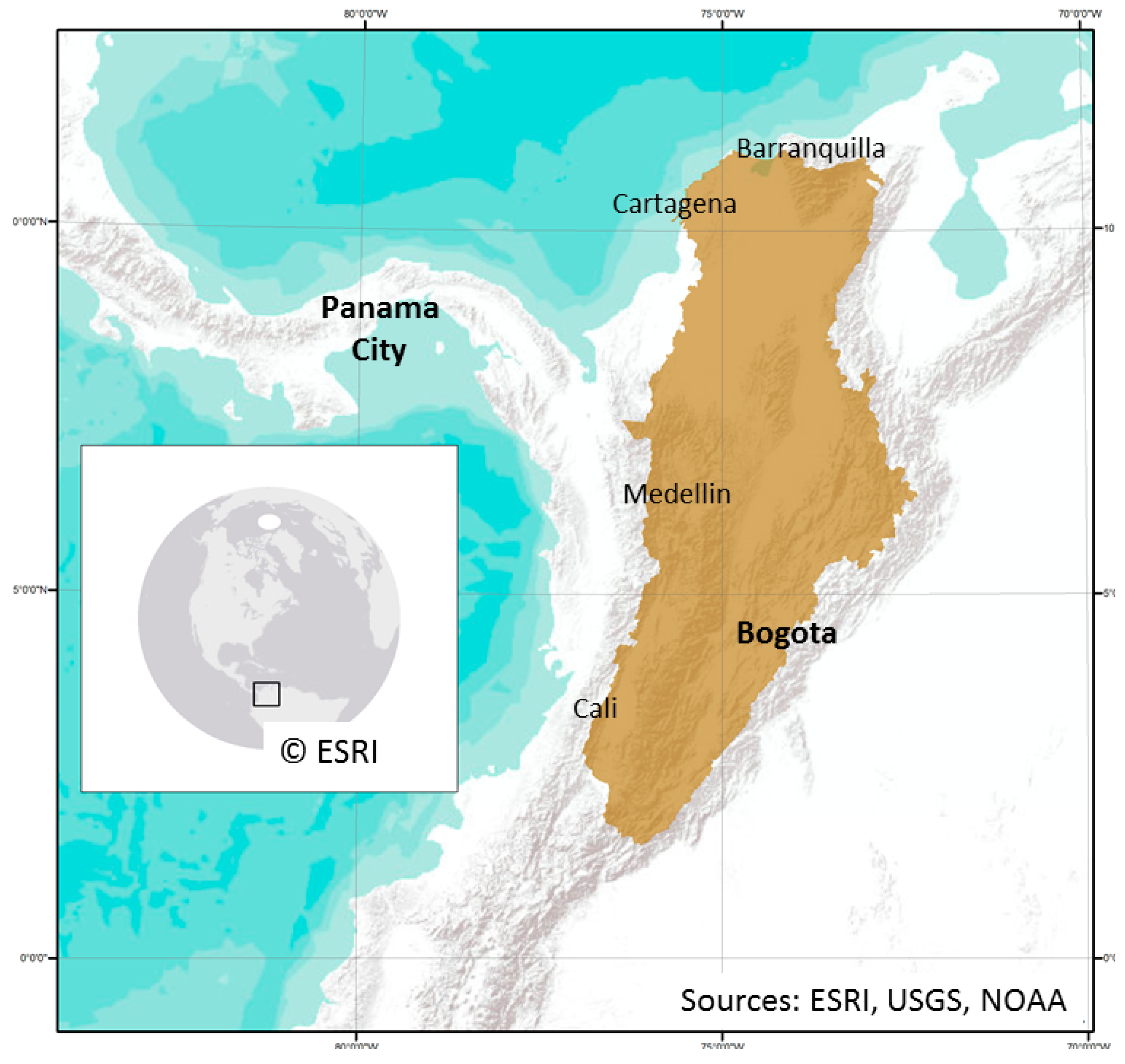
The Magdalena River watershed, highlighted in Figure 1, is an area of central Colombia that is 273,048 km2 in size, which makes it slightly larger than the State of Colorado. It is located between 1°32′N to 11°7′N and 72°19′W to 77°0′W. The Magdalena River watershed is relatively isolated by the coastline to the north and the Andean mountains to the south. This contained area makes the Magdalena River watershed well-suited to the study of the host-vector relationship as it reduces the opportunity for species dispersion from confounding external influence [24].
2.2. Data Sources
Data on Dengue fever cases were collected, processed, and confirmed by the INS according to its protocols [25]. The researchers downloaded them from the INS site [6]. This study used confirmed cases of DF by municipality for each of the three study years.
Population data were downloaded from the 2005 General Census administered by the National Administrative Department of Statistics (Departamento Administrativo Nacional de Estadística, DANE) [26] and projected to 2012–2014 levels by the data proprietors.
Remote sensing data were acquired from the National Aeronautics and Space Administration (NASA) data servers at various resolutions for each day of the study period. This included the Moderate Resolution Imaging Spectroradiometer (MODIS) satellite products, the Tropical Rainfall Measuring Mission (TRMM) 3B42 product, and the Shuttle Radar Topography Mission (SRTM) product.
2.3. Explanatory Variables
The Land Surface Temperature (LST)/Emissivity Daily L3 Global (MYD11A1) product at 1 km resolution, supplied both daytime and nighttime land surface temperature (LST), which was processed to reflect Celsius temperatures. The Surface Reflectance Daily L2G Global (MYD09GQ) product at 250 m resolution was used to derive the two-band Enhanced Vegetation Index as outlined in the MODIS Vegetation Index User’s Guide [27]. It was planned to calculate the Normalized Difference Vegetation Index (NDVI), but because of the high biomass of the region the backup enhanced vegetation index (EVI) was used. The preference for using EVI was due to better de-coupling of the canopy background and gave better results than did the NDVI [27]. The Tropical Rainfall Measuring Mission (TRMM) imagery was used to estimate precipitation. The TRMM imagery is provided globally at approximately 16 km spatial resolution and was clipped down to the study region for faster processing. Because the health data were reported weekly using the ISO Week Date format, the above environmental variables were all composited using the same schedule. Because the imagery was gathered by satellites, clouds can mask portions of each image. Combining several daily image files into one composite image reduced the area of the resulting image that was covered by clouds. Also, the daily images were combined based on the same weekly periods as the health data were collected so that trends could be explored.
2.4. Data Preprocessing
The weekly imagery for each variable was aggregated using the ArcGIS 10.3 Spatial Analyst Tool Cell Statistics [28]. This aggregated each variable to the annual minimum, maximum, and mean for a raster cell. This imagery was then aggregated to the municipality level using the Spatial Analyst tool, Zonal Statistics as Table, again for minimum, maximum, and mean. As an example, the minimum daytime LST for the municipality from all mean annual daytime LST could be represented. This allowed for a much finer resolution of the environmental variables over simply the minimum, maximum, and mean alone.
Since land use and elevation change very little over time, only a single instance of each was obtained. The MODIS MCD12Q1 imagery was used to ascertain land use and land cover (LULC). This composite image was separated into independent images, one for each classification outlined on the products website [29]. This resulted in separate images, at 500 m resolution, for barren, cropland, forest, savanna, shrubland, snow and ice, urban, and wetland. Elevation imagery was obtained from the Shuttle Radar Topography Mission at 30 m resolution. The elevation imagery was not masked to 1800 m above sea level, as is suggested by other studies [22], to investigate the previously held assumption that the vector cannot survive at higher elevations. In fact, its presence has been recently reported at an elevation of 2302 m ASL in Colombia [30]. Besides climate change, other factors may support the possibility of finding this mosquito outside of its assumed range. Highly urbanized areas may provide conditions that attenuate environmental effects, such as the urban heat island effect and access to sewers. For example, Washington, D.C., which is well outside the supposed temperature range of Ae. Aegypti, experiences micro-habitats under the city with year-round conditions favorable to the vector [31].
2.5. Boosted Regression Tree Analysis
The Boosted Regression Tree (BRT) model utilizes an initial regression tree and then improves upon it in a forward stage-wise manner (boosting) repetitively so that unexplained variation in the responses at each stage are minimized [32,33,34]. The BRT is less prone to over-fitting through its use of cross-validation when used to fit complex functions. Over-fitting can be seen as a failure of the algorithm to ‘stop’ once a balance between predictive performance and model fit has been optimized [33]. This and other reasons have made the BRT method useful in previous studies which successfully mapped DF, along with other vector-borne diseases, and the Aedes mosquito vector itself [4,16,35,36], usually in small select areas of countries such as Malaysia [18] and Singapore [37].
The BRT analysis was conducted twice: once using the Bernoulli family of presence/absence and again using the Poisson family of actual case counts. In the first analysis, any municipality reporting one or more cases of DF in the year was coded as having disease “presence”, while all others were coded as not having disease presence (“absence”). Following Elith et al. [33] and the provided functions, and using the statistical package R with the gbm package (https://www.r-project.org), the BRT model was run for each year in the data with 64 explanatory variables (see Appendix A for complete list) against the outcome (disease presence/absence). Each model for each year was fitted using a tree.complexity of 5, a bag.fraction of 0.75, and a learning.rate which was adjusted down to 0.004 so that an average of 1000 trees were built. Following Cheong et al. [18], the model was run 100 times and the mean for all 100 runs was calculated. The relative influence plot was then used and the cutoff value calculated as 100/64 = 1.5625. The BRT model was then run again with only those explanatory variables having a relative influence value above the cutoff value. Additionally, 25 percent of the data was set aside as a testing set to test the ability of the model for each year.
In the second analysis, the reported cases of DF were used in the same model as for the Bernoulli family. The only change to the models consisted of replacing family = “Bernoulli” with family = “poisson”. The dependent variable column was set as the quantity of reported DF cases within the municipality. The Poisson family was chosen since the count data are highly skewed. Each model was again fitted using a tree.complexity of 5, a bag.fraction of 0.75, and a learning.rate adjusted down to 0.004. The same settings were used to reduce differences in the two models and to make comparison straightforward. We did not tune the Poisson model in order to maintain comparability with the Bernoulli model.
3. Results
The metrics package in R was used to calculate the RMSE between the predicted mean and actual cases in the training data, along with the Pearson correlation coefficient and p-value. The results are summarized in Table 1, and show that the Poisson family out-performed the Bernoulli family models across all years. The average RMSE for all three years was also considerably lower for the Poisson model (mean = 28.267) compared to the Bernoulli model (mean = 98.732), reflecting a better model fit.
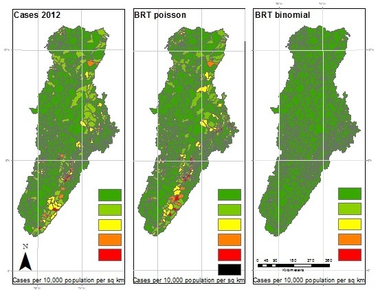
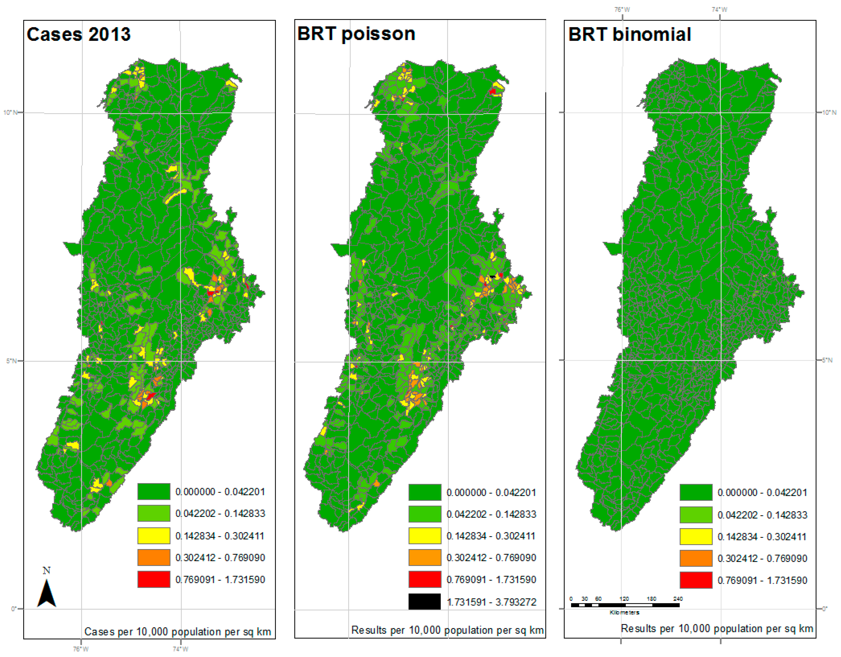
The maps shown in Figure 2, Figure 3 and Figure 4 reflect the results shown in Table 1. The left panel represents the cases per 10,000 population per square kilometer for each municipality by year. The dark green color represents very low ratios of DF, and red color reflects a higher incidence of DF. All maps used the same classification as the reported cases map for comparison, with an additional symbol (black) used for values outside the reported cases range. The center panel represents the results of the BRT analysis using the Poisson family, while the right panel represents the results of the BRT analysis using the Bernoulli family, or presence/absence data. While the BRT Poisson map reflects a higher correlation and lower RMSE to the reported cases than the BRT Binomial map, there is still some apparent underfitting of the model.
Those areas in the central and southern sections of the watershed, along the foothills between mountain ranges, show an expected coincidence between high levels of DF cases and high estimated probability of DF occurrence. As expected, the areas, where low probability of occurrence coincided with low cases, also coincided with the higher elevation areas of the watershed. As previously noted, elevation was shown to be a limiting factor in the spread of DF by Ae. aegypti.
The 20 relative importance variables for each year are listed in Table 2, with population density (POP_DEN), daytime LST minimum annual maximum municipality variables (LD1B) ranking high in both models. In the Poisson models population density or daytime LST mean annual maximum municipality (LD3B) represented more than 50% of the relative influence in a year, whereas there was no such clear distinction in the Bernoulli models. Nighttime temperatures (LNxy) were more common in the Bernoulli models along with mean elevation (EL3). Population density within a municipality was a significant variable across all models for all years.
4. Discussion
Using boosted regression tree analysis within the Magdalena River watershed of Colombia as a study site, this paper sets out to identify environmental factors with high relative influence of DF incidence and to map the spatial distribution of DF risk. A comparison was also made between the standard presence/absence models found in the literature with a model that used the reported case counts by municipality. The results show that the interaction between population density, elevation, daytime LST, and nighttime LST played the most descriptive role in determining the niche of DF within this study. Population density was one of the highest relative influence variables across all of the years studied. This strong positive relationship can be explained by several factors, such as the preference of Ae. aegypti to breed in water filled artificial containers associated with human activity [38], which may be more abundant and closer to higher occurrences of human population density. In addition, greater population density means more opportunity for the mosquito to transmit the virus from an infected person to an uninfected one [39].
A strong influence from elevation was expected due to the previously established inverse relationship between elevation and temperature in connection to the widely-reported influence of temperature on Ae. aegypti survival [5,40,41] and Dengue transmission [24]. In a study conducted in Central Mexico, Moreno-Madriñán et al. [8] used RS technology to detect a strong inverse relationship (supporting previously used in situ measurement studies) between elevation and Ae. aegypti abundance. However, in the present study, a strong influence from Mean elevation (EL3) was observed in the Bernoulli models, but not in the Poisson models. Assuming the Poisson models were indeed more accurate, a possible low influence from elevation may be related to the fact that most of the large cities and the most populated areas are located at higher elevations due to cultural habits in this region. As explained previously, population density was among the most influential variables, thus this cultural habit could have confounded the effect of elevation in this study area. In addition, urban heat island effect might have played a role in these large cities. Many cases reported at higher elevations may have been brought in by people traveling from other municipalities located at lower elevations. Indeed, several authors estimated an elevation limit for Ae. aegypti to be between 1800 m ASL and 2000 m ASL [22]. In Mexico, Lozano-Cifuentes et al. [42] reported Ae. aegypti rare but present at an elevation of 2130 m ASL while it had been previously reported at 1630 m ASL [43]. In Colombia, the highest elevation previously reported was 2200 m ASL [44], with a more recent report having found evidence above 2300 m ASL [30]. In the data supplied for 2013, there were 15 municipalities above 2300 m ASL that listed one or more cases of DF.
Due to the aggregation of the environmental variables, several highly correlated sub-variables were generated and used. All raster pixels falling within a municipality border were aggregated to create a minimum, maximum, and mean temperature assigned to that municipality. In a linear or logistic regression analysis this would be a problem, but the BRT method used herein is a decision tree method with cross-validation, and was able to overcome this limitation by using many weak classifiers to create a stronger classifier [33].
The Poisson models consistently showed daytime LST to be highly determinant variables, which is also in line with other literature that model mosquito habitat and in particular temperature in relation to disease [40,45,46]. Daytime LST appear to be a more important limiting factor as compared with nighttime LST, probably because the highest temperatures reached in many areas of this tropical site can easily exceed the upper limit of the comfort window for Ae. aegypti and would be expected to be reached during the day. It is important to mention that Stanforth et al. [46] detected, as anticipated, respectively positive and negative relationships of DF to temperature and elevation, using the same data set as this study but with a principal component analysis methodology.
While precipitation has been considered significant in other studies [37], here precipitation did not have a significant relative influence. Stanforth et al. [46] also detected a relatively low influence of precipitation. Such a low role of precipitation might be explained by the domestic and peri-domestic environment that Ae. aegypti prefers [47], in which there is an abundance of larval rearing sites filled with water by humans (i.e., water storage tanks, flower pots) [39], thus making its reproduction less dependent on precipitation. Accordingly, it has been suggested that the strong dependency of this mosquito on water containers filled by humans, makes it less susceptible to rain variability [19]. This may also explain why Stanforth et al. [46] found a negative association between the minimum annual precipitation and dengue incidence. Suggesting people may be more likely to store water during a dry season, providing more opportunities for larval rearing while on the contrary the faster surface water flow during the rainy season may not allow time for larval development [47].
All other variables were below the significance threshold, notably including all the land use and land cover variables (LULC). The latter was an unexpected finding since other studies, e.g., [18], have reported LULC variables to be useful in determining the risk of DF. The discrepancy may be due to the greater number of variables and sub-variables used in our models. For instance, sub-variables of LST showed to be more important than LULC, potentially minimizing the combined effect of LULC. In addition, Cheong et al. [18] only used LULC variables, so the weight of their LULC index could not be outperformed in their model by stronger variables—e.g., temperature—as was experienced in this study. The small amount of any one type of land use in a given municipality compared to the satellite coverage of the entire area for other variables, such as LST, may also have overshadowed the contribution of LULC variables. It is noteworthy that ‘Urban’ was not as determinant a variable, despite the known affinity of the vector for urban areas. This may be due to ‘Urban’ derived from satellite imagery representing all impervious surfaces, such as roads, rooftops, and sidewalks, and other areas the vector could not use for breeding sites.
As discussed previously in Table 1, the Poisson models had a lower RMSE and higher correlation over the study period than the Bernoulli models. Additionally, the Poisson models used actual cases reported for each municipality, thereby giving a more accurate picture of the spatial distribution of DF in the Magdalena River watershed. Generally, the municipalities in the central and southern sections of the watershed along the valleys between mountain ranges show an expected coincidence between high levels of DF cases and high estimated probability of risk. Likewise, as expected, the municipalities with low probability of occurrence generally coincided with low numbers of actual cases. While the models show a high correlation to the dependent variables, there was still some under-fitting and over-fitting occurring. In the case of the Bernoulli models, factors that influence this could be due in part to a limitation of the current model that can only accept a binary dependent variable, the presence or absence of DF cases, rather than the actual counts of DF for each municipality. Another reason for this could be the interaction and interdependence of the tree complexity, bagging fraction, and learning rate [48].
Another strength of the BRT models described here is in the output of a map of the likelihood of DF prevalence on a municipality level. Not only is this method less computationally intensive, but it allows for a more identifiable and user-friendly result for end users that may not be as familiar with other types of maps or analysis results. Since the model uses aggregated municipality data, this method is also easier for those that may not be able to use identifiable patient data to get reliable and useful results. Future research could consider using the method outlined here as a first step to identify municipalities at high risk, and then follow up using data fusion and higher resolution analysis methods, along with the same environmental data presented here.
Studies, such as Cheong et al. [18], use geocoded point locations of reported cases of DF. In this research, only weekly counts by municipality were available, which is a limitation in many cases, but it makes this method easier and more accessible to researchers without advanced computing capability or access to geocoded disease data. Being able to use readily available municipality shapefiles and standardized weekly reporting would allow this method to be adopted by a larger group of public health practitioners in more areas, especially those in developing countries or those with less geospatial analysis experience.
As DF is an endemic disease in the Magdalena River watershed of Colombia, the effect of asymptomatic infection rate and reporting bias may also play a role in the ability of the models [35]. Due to the aggregation of all cases into a year, this could bias the ability of the model by including municipalities with misreported cases. However, such possible bias may be neutralized in follow-up studies with higher temporal resolution, where municipalities with few cases are also more likely to have frequent reports of absence while those with high numbers of cases are more likely to frequently be reported with presence.
5. Conclusions
This study has shown that boosted regression tree analysis can be used as a tool in the ecological niche modeling of DF in the Magdalena River watershed of Colombia. By using readily available and freely accessible data, we have shown that practitioners both within and outside of Colombia can quickly create accurate maps of annual DF incidence. Furthermore, our study has shown that population density (POP_DEN) plays a strong role in the modeling of DF in our study area, along with the satellite-derived variables of mean annual LST, especially daytime. The methods described here could also be extended to other regions and diseases, making it useful to a wide range of end users. Another benefit of this study is in the comparison between using the functions created by Elith et al. [33] and the gbm package in R, and extending them beyond the Bernoulli family of models. Using the same methods and functions outlined in existing literature for the presence/absence models, this study showed that they can be extended and used with actual cases of disease reported, giving a clearer picture of the spatial distribution of infection.
It should also be mentioned that a limitation of the study is in the idea of human movement from one municipality to another. Future research should take into account socioeconomic vulnerabilities, such as those used in the study of Cali, Colombia by Hagenlocher et al. [49] in conjunction with the variables identified herein to broaden the scope of the risk assessment. Along with human movement and socioeconomic vulnerabilities, running the data on weekly reports of DF, and then creating a method to predict the number of cases generated from the risk analysis could be incorporated into an early warning system for disease outbreaks.
Acknowledgments
This study was supported by the IUPUI Chancellor for Research—Research Support Funds Grant. The study was also possible because of the accessibility to public health data made available by the National Institute of Health (Instituto Nacional de Salud, INS) of Colombia. The authors would like to thank Mary Lefevers for her assistance in the data preprocessing and Victor E. Casallas-Bedoya from INS for his assistance with data information. The authors would also like to thank the reviewers for their insights and suggestions.
Author Contributions
J.A. participated in the research design, data collection, analysis and interpretation, and preparation of the manuscript. M.M. participated in the research design, data collection, analysis, interpretation, and conceived the idea of this study. C.Y. guided the statistical analysis. A.S. participated in the research design, data collection, analysis, and interpretation. All authors reviewed and approved the manuscript.
Conflicts of Interest
The authors declare no conflict of interest.
Appendix A
Codebook
Variable naming format XXYZ, where XX is two-letter designation of variable, Y is a numeric designation for minimum, maximum, or mean, of the cell statistics for the annual period, and Z is an alphanumeric designator for the minimum, maximum, or mean of the zonal statistics. Land Cover variables only have an XXY format due to only being a single dataset and not a weekly compilation.
Example LN1A would be the Nighttime LST value for the minimum cell statistics for the whole year and the minimum zonal statistic for the whole municipality.
| Variable | XX | Y | Z |
| LST Night | LN | Min is 1 | Min is A |
| LST Day | LD | Max is 2 | Max is B |
| Precipitation | PR | Mean is 3 | Mean is C |
| Vegetation | VE | ||
| Elevation | EL | ||
| Land Cover–Barren | BA | ||
| Land Cover–Cropland | CR | ||
| Land Cover–Forest | FO | ||
| Land Cover–Savanna | SA | ||
| Land Cover–Shrubland | SH | ||
| Land Cover–Snowice | SN | ||
| Land Cover–Urban | UR | ||
| Land Cover–Wetland | WE | ||
| Population Density | POP_DEN |
| Code | Description |
| BA1 | barren minimum municipality |
| BA2 | barren maximum municipality |
| BA3 | barren mean municipality |
| CR1 | cropland minimum municipality |
| CR2 | cropland maximum municipality |
| CR3 | cropland mean municipality |
| EL1 | elevation minimum municipality |
| EL2 | elevation maximum municipality |
| EL3 | elevation mean municipality |
| FO1 | forest minimum municipality |
| FO2 | forest maximum municipality |
| FO3 | forest mean municipality |
| LD1A | daytime LST minimum annual minimum municipality |
| LD1B | daytime LST minimum annual maximum municipality |
| LD1C | daytime LST minimum annual mean municipality |
| LD2A | daytime LST maximum annual minimum municipality |
| LD2B | daytime LST maximum annual maximum municipality |
| LD2C | daytime LST maximum annual mean municipality |
| LD3A | daytime LST mean annual minimum municipality |
| LD3B | daytime LST mean annual maximum municipality |
| LD3C | daytime LST mean annual mean municipality |
| LN1A | nighttime LST minimum annual minimum municipality |
| LN1B | nighttime LST minimum annual maximum municipality |
| LN1C | nighttime LST minimum annual mean municipality |
| LN2A | nighttime LST maximum annual minimum municipality |
| LN2B | nighttime LST maximum annual maximum municipality |
| LN2C | nighttime LST maximum annual mean municipality |
| LN3A | nighttime LST mean annual minimum municipality |
| LN3B | nighttime LST mean annual maximum municipality |
| LN3C | nighttime LST mean annual mean municipality |
| POP_DEN | population density |
| PR1A | precipitation minimum annual minimum municipality |
| PR1B | precipitation minimum annual maximum municipality |
| PR1C | precipitation minimum annual mean municipality |
| PR2A | precipitation maximum annual minimum municipality |
| PR2B | precipitation maximum annual maximum municipality |
| PR2C | precipitation maximum annual mean municipality |
| PR4A | precipitation total annual minimum municipality |
| PR4B | precipitation total annual maximum municipality |
| PR4C | precipitation total annual mean municipality |
| SA1 | savannah minimum municipality |
| SA2 | savannah maximum municipality |
| SA3 | savannah mean municipality |
| SH1 | shrubland minimum municipality |
| SH2 | shrubland maximum municipality |
| SH3 | shrubland mean municipality |
| SN1 | snow and ice minimum municipality |
| SN2 | snow and ice maximum municipality |
| SN3 | snow and ice mean municipality |
| UR1 | urban minimum municipality |
| UR2 | urban maximum municipality |
| UR3 | urban mean municipality |
| VE1A | vegetation minimum annual minimum municipality |
| VE1B | vegetation minimum annual maximum municipality |
| VE1C | vegetation minimum annual mean municipality |
| VE2A | vegetation maximum annual minimum municipality |
| VE2B | vegetation maximum annual maximum municipality |
| VE2C | vegetation maximum annual mean municipality |
| VE3A | vegetation mean annual minimum municipality |
| VE3B | vegetation mean annual maximum municipality |
| VE3C | vegetation mean annual mean municipality |
| WE1 | wetland minimum municipality |
| WE2 | wetland maximum municipality |
| WE3 | wetland mean municipality |
References
- Meentemeyer, R.K.; Haas, S.E.; Vaclavik, T. Landscape epidemiology of emerging infectious diseases in natural and human-altered ecosystems. Annu. Rev. Phytopathol. 2012, 50, 379–402. [Google Scholar] [CrossRef] [PubMed]
- Dengue. Available online: http://www.cdc.gov/dengue/index.html (accessed on 10 August 2016).
- Kaushal, M. Epidemiology of Dengue. Available online: http://www.slideshare.net/menaalkaushal/dengue-epidemiology-case-management-26937383 (accessed on 3 August 2016).
- Messina, J.P.; Kraemer, M.U.; Brady, O.J.; Pigott, D.M.; Shearer, F.M.; Weiss, D.J.; Golding, N.; Ruktanonchai, C.W.; Gething, P.W.; Cohn, E.; et al. Mapping global environmental suitability for Zika virus. eLife 2016, 5, e15272. [Google Scholar] [CrossRef] [PubMed]
- Castro Rodriguez, R.; Carrasquilla, G.; Porras, A.; Galera-Gelvez, K.; Lopez Yescas, J.G.; Rueda-Gallardo, J.A. The Burden of Dengue and the Financial Cost to Colombia, 2010–2012. Am. J. Trop. Med. Hyg. 2016, 94, 1065–1072. [Google Scholar] [CrossRef] [PubMed]
- Instituto Nacional de Salud (INS) Programa SIVIGILA. Entidad Adscrita al Ministerio de Salud y Protección Social de Colombia. 2014. Available online: http://www.ins.gov.co/lineas-de-accion/Subdireccion-Vigilancia/sivigila/Paginas/vigilancia-rutinaria.aspx (accessed on 12 August 2016).
- Hay, S.I. An overview of remote sensing and geodesy for epidemiology and public health application. Adv. Parasitol. 2000, 47, 1–35. [Google Scholar] [PubMed]
- Moreno-Madriñán, M.; Crosson, W.; Eisen, L.; Estes, S.; Estes, M., Jr.; Hayden, M.; Hemmings, S.; Irwin, D.; Lozano-Fuentes, S.; Monaghan, A.; et al. Correlating remote sensing data with the abundance of pupae of the dengue virus mosquito vector, Aedes aegypti, in central Mexico. ISPRS Int. J. Geo-Inf. 2014, 3, 732–749. [Google Scholar] [CrossRef]
- Machault, V.; Yébakima, A.; Etienne, M.; Vignolles, C.; Palany, P.; Tourre, Y.M.; Guérécheau, M.; Lacaux, J.P. Mapping entomological dengue risk levels in Martinique using high-resolution remote-sensing environmental data. ISPRS Int. J. Geo-Inf. 2014, 3, 1352–1371. [Google Scholar] [CrossRef]
- Aertsen, W.; Kint, V.; de Vos, B.; Deckers, J.; van Orshoven, J.; Muys, B. Predicting forest site productivity in temperate lowland from forest floor, soil and litterfall characteristics using boosted regression trees. Plant Soil 2012, 354, 157–172. [Google Scholar] [CrossRef]
- Carty, D.; Young, T.; Zaretzki, R.; Petutschnigg, A. Predicting and Correlating the Strength Properties of Wood Composite Process Parameters by Use of Boosted Regression Tree Models. For. Prod. J. 2015, 65, 365–371. [Google Scholar] [CrossRef]
- Shah, D.A.; De Wolf, E.D.; Paul, P.A.; Madden, L.V. Predicting Fusarium Head Blight Epidemics with Boosted Regression Trees. Phytopathology 2014, 104, 702–714. [Google Scholar] [CrossRef] [PubMed]
- De’Ath, G.; Fabricius, K.E. Classification and regression trees: A powerful yet simple technique for ecological data analysis. Ecology 2000, 81, 3178–3192. [Google Scholar] [CrossRef]
- Friedman, J.H.; Meulman, J.J. Multiple additive regression trees with application in epidemiology. Stat. Med. 2003, 22, 1365–1381. [Google Scholar] [CrossRef] [PubMed]
- Lawrence, R.; Bunn, A.; Powell, S.; Zambon, M. Classification of remotely sensed imagery using stochastic gradient boosting as a refinement of classification tree analysis. Remote Sens. Environ. 2004, 90, 331–336. [Google Scholar] [CrossRef]
- Pigott, D.M.; Bhatt, S.; Golding, N.; Duda, K.A.; Battle, K.E.; Brady, O.J.; Messina, J.P.; Balard, Y.; Bastien, P.; Pratlong, F.; et al. Global distribution maps of the leishmaniases. eLife 2014, 3, e35671. [Google Scholar] [CrossRef] [PubMed]
- Messina, J.P.; Pigott, D.M.; Golding, N.; Duda, K.A.; Brownstein, J.S.; Weiss, D.J.; Gibson, H.; Robinson, T.P.; Gilbert, M.; William Wint, G.R.; et al. The global distribution of Crimean-Congo hemorrhagic fever. Trans. R. Soc. Trop. Med. Hyg. 2015, 109, 503–513. [Google Scholar] [CrossRef] [PubMed]
- Cheong, Y.L.; Leitão, P.J.; Lakes, T. Assessment of land use factors associated with dengue cases in Malaysia using boosted regression trees. Spat. Spatiotemporal. Epidemiol. 2014, 10, 75–84. [Google Scholar] [CrossRef] [PubMed]
- Gubler, D.J. Dengue, Urbanization and Globalization: The Unholy Trinity of the 21(st) Century. Trop. Med. Health 2011, 39, 3–11. [Google Scholar] [CrossRef] [PubMed]
- Chareonviriyaphap, T.; Akratanakul, P.; Nettanomsak, S.; Huntamai, S. Larval habitats and distribution patterns of Aedes aegypti (Linnaeus) and Aedes albopictus (Skuse), in Thailand. Southeast. Asian J. Trop. Med. Public Health 2003, 34, 529–535. [Google Scholar] [PubMed]
- Wan-Norafikah, O.; Nazni, W.A.; Noramiza, S.; Shafa’ar-Ko’ohar, S.; Heah, S.K.; Nor-Azlina, A.H.; Khairul-Asuad, M.; Lee, H.L. Distribution of Aedes mosquitoes in three selected localities in Malaysia. Sains Malays. 2012, 41, 1309–1313. [Google Scholar]
- Delmelle, A.P.E.; Kanaroglou, P. (Eds.) Spatial Analysis in Health Geography; Ashgate Publishing, Ltd.: Farnham, UK, 2015. [Google Scholar]
- Heymann, D.L. Control of Communicable Diseases Manual; American Public Health Association: Washington, DC, USA, 2008. [Google Scholar]
- Morin, C.W.; Comrie, A.C.; Ernst, K. EHP—Climate and Dengue Transmission: Evidence and Implications. Environ. Health Perspect. 2013, 1264, 1264–1272. [Google Scholar]
- De la Hoz, F.; Martínez-Duran, M.; Pacheco-García, O.; Quijada-Bonilla, H. Protocolo de Vigilancia en Salud Pública: Dengue. In Public Health Surveillance Protocol. Dengue; Instituto Nacional de Salud: Bogotá, Colombia, 2014. [Google Scholar]
- Departamento Administrativo Nacional de Estadística (DANE). Gobierno de Colombia. 2014. Available online: http://www.dane.gov.co/ (accessed on 19 July 2014).
- Ramon Solano, R.; Didan, K.; Jacobson, A.; Huete, A. Modis Vegetation Index User’s Guide; The University of Arizona: Tucson, AZ, USA, 2010. [Google Scholar]
- ArcGIS for Desktop. Available online: http://www.esri.com/software/arcgis/arcgis-for-desktop (accessed on 3 November 2016).
- LP DAAC: NASA Land Data Products and Services. Land Cover Type Yearly L3 Global 500 m SIN Grid. Available online: https://lpdaac.usgs.gov/dataset_discovery/modis/modis_products_table/mcd12q1 (accessed on 5 November 2016).
- Ruiz-Lopez, F.; Gonzalez-Mazo, A.; Velez-Mira, A.; Gomez, G.F.; Zuleta, L.; Uribe, S.; Velez-Bernal, I.D. Presence of Aedes (Stegomyia) aegypti (Linnaeus, 1762) and its natural infection with dengue virus at unrecorded heights in Colombia. Biomedica 2016, 36, 303–308. [Google Scholar] [CrossRef] [PubMed]
- Lima, A.; Lovin, D.D.; Hickner, P.V.; Severson, D.W. Evidence for an overwintering population of Aedes aegypti in Capitol Hill Neighborhood, Washington, DC. Am. J. Trop. Med. Hyg. 2016, 94, 231–235. [Google Scholar] [CrossRef] [PubMed]
- Friedman, J.H. Greedy function approximation: A gradient boosting machine. Statistics 2011, 29, 1189–1232. [Google Scholar] [CrossRef]
- Elith, J.; Leathwick, J.R.; Hastie, T. A working guide to boosted regression trees. J. Anim. Ecol. 2008, 77, 802–813. [Google Scholar] [CrossRef] [PubMed]
- Leathwick, J.R.; Elith, J.; Francis, M.P.; Hastie, T.; Taylor, P. Variation in demersal fish species richness in the oceans surrounding New Zealand: An analysis using boosted regression trees. Mar. Ecol. Prog. Ser. 2006, 321, 267–281. [Google Scholar] [CrossRef]
- Bhatt, S.; Gething, P.W.; Brady, O.J.; Messina, J.P.; Farlow, A.W.; Moyes, C.L.; Drake, J.M.; Brownstein, J.S.; Hoen, A.G.; Sankoh, O.; et al. The global distribution and burden of dengue. Nature 2013, 496, 504–507. [Google Scholar] [CrossRef] [PubMed]
- Kraemer, M.U.G.; Sinka, M.E.; Duda, K.A.; Mylne, A.Q.N.; Shearer, F.M.; Barker, C.M.; Moore, C.G.; Carvalho, R.G.; Coelho, G.E.; Van Bortel, W.; et al. The global distribution of the arbovirus vectors Aedes aegypti and Ae. Albopictus. eLife 2015, 4, 1–18. [Google Scholar] [CrossRef] [PubMed]
- Shi, Y.; Liu, X.; Kok, S.-Y.; Rajarethinam, J.; Liang, S.; Yap, G.; Chong, C.-S.; Lee, K.-S.; Tan, S.S.Y.; Chin, C.K.Y.; et al. Three-Month Real-Time Dengue Forecast Models: An Early Warning System for Outbreak Alerts and Policy Decision Support in Singapore. Environ. Health Perspect. 2015. [Google Scholar] [CrossRef] [PubMed]
- Dhang, C.; Benjamin, S.; Saranum, M.; Fook, C.; Lim, L.; Ahmad, N.; Sofian-Azirun, M. Dengue vector surveillance in urban residential and settlement areas in Selangor, Malaysia. Trop. Biomed. 2005, 22, 39–43. [Google Scholar]
- Lounibos, L.P. Invasions by insect vectors of human disease. Annu. Rev. Entomol. 2002, 47, 233–266. [Google Scholar] [CrossRef] [PubMed]
- Brady, O.J.; Golding, N.; Pigott, D.M.; Kraemer, M.U.G.; Messina, J.P.; Reiner, R.C.; Scott, T.W.; Smith, D.L.; Gething, P.W.; Hay, S.I. Global temperature constraints on Aedes aegypti and Ae. Albopictus persistence and competence for dengue virus transmission. Parasites Vectors 2014, 7, 338. [Google Scholar] [CrossRef] [PubMed]
- Rueda, L.; Patel, K.; Axtell, R.; Stinner, R. Temperature-Dependent Development and Survival Rates of Culex quinquefasciatus and Aedes aegypti. J. Med. Entomol. 1990, 27, 892–898. [Google Scholar] [CrossRef] [PubMed]
- Lozano-Fuentes, S.; Hayden, M.H.; Welsh-Rodriguez, C.; Ochoa-Martinez, C.; Tapia-Santos, B.; Kobylinski, K.C.; Uejio, C.K.; Zielinski-Gutierrez, E.; Delle Monache, L.; Monaghan, A.J.; et al. The dengue virus mosquito vector Aedes aegypti at high elevation in México. Am. J. Trop. Med. Hyg. 2012, 87, 902–909. [Google Scholar] [CrossRef] [PubMed]
- Ibanez-Bernal, S. New altitudinal record of Aedes(Stegomyia) aegypti(Linnaeus, 1762)(Diptera: Culicidae) in Mexico.). Folia Entomol. Mex. 1987, 72, 163–164. [Google Scholar]
- Suárez, M.F.; Nelson, M.J. Registro de altitud del Aedes aegypti en Colombia. Biomédica 1981, 1, 225. [Google Scholar] [CrossRef]
- Rogers, D.J.; Wilson, A.J.; Hay, S.I.; Graham, A.J. The global distribution of yellow fever and dengue. Adv. Parasitol. 2006, 62, 181–220. [Google Scholar] [PubMed]
- Stanforth, A.; Moreno-Madriñán, M.J.; Ashby, J. Exploratory Analysis of Dengue Fever Niche Variables within the Rio Magdalena Watershed. Remote Sens. 2016, 8, 770. [Google Scholar] [CrossRef]
- Moreno-Madriñán, M.J.; Turell, M.J. Factors of concern regarding Zika and other Aedes aegypti-transmitted viruses in the U.S. J. Med. Entomol. 2017. [Google Scholar] [CrossRef]
- Ridgeway, G. Generalized Boosted Models: A Guide to the gbm Package. 2007. Available online: http://www.saedsayad.com/docs/gbm2.pdf (accessed on 3 August 2007).
- Hagenlocher, M.; Delmelle, E.; Casas, I.; Kienberger, S. Assessing socioeconomic vulnerability to dengue fever in Cali, Colombia: Statistical vs expert-based modeling. Int. J. Health Geogr. 2013, 12, 36. [Google Scholar] [CrossRef] [PubMed]
Figure 1.
Magdalena River watershed (shaded).

Figure 2.
Results of 2012 analysis—The left panel represents the reported cases per 10,000 population per square kilometer for each municipality. The center panel represents the results of the BRT analysis using the Poisson family, while the right panel represents the results of the BRT analysis using the Bernoulli family. The dark green color represents very low ratios of DF, and red color reflects a higher incidence of DF. All maps used the natural breaks classification set to five classes for comparison.
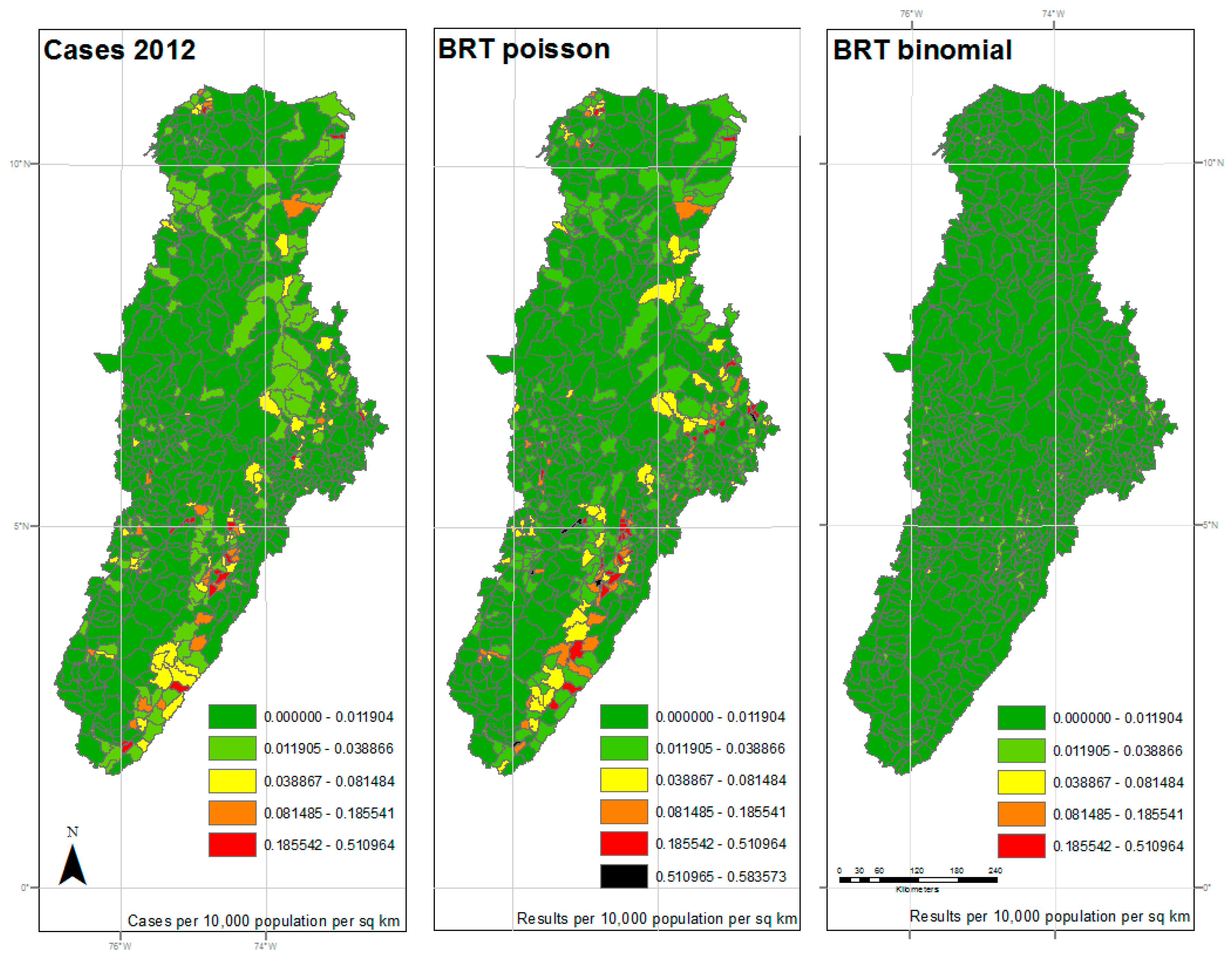
Figure 3.
Results of 2013 analysis—The left panel represents the reported cases per 10,000 population per square kilometer for each municipality. The center panel represents the results of the BRT analysis using the Poisson family, while the right panel represents the results of the BRT analysis using the Bernoulli family. The dark green color represents very low ratios of DF, and red color reflects a higher incidence of DF. All maps used the natural breaks classification set to five classes for comparison.

Figure 4.
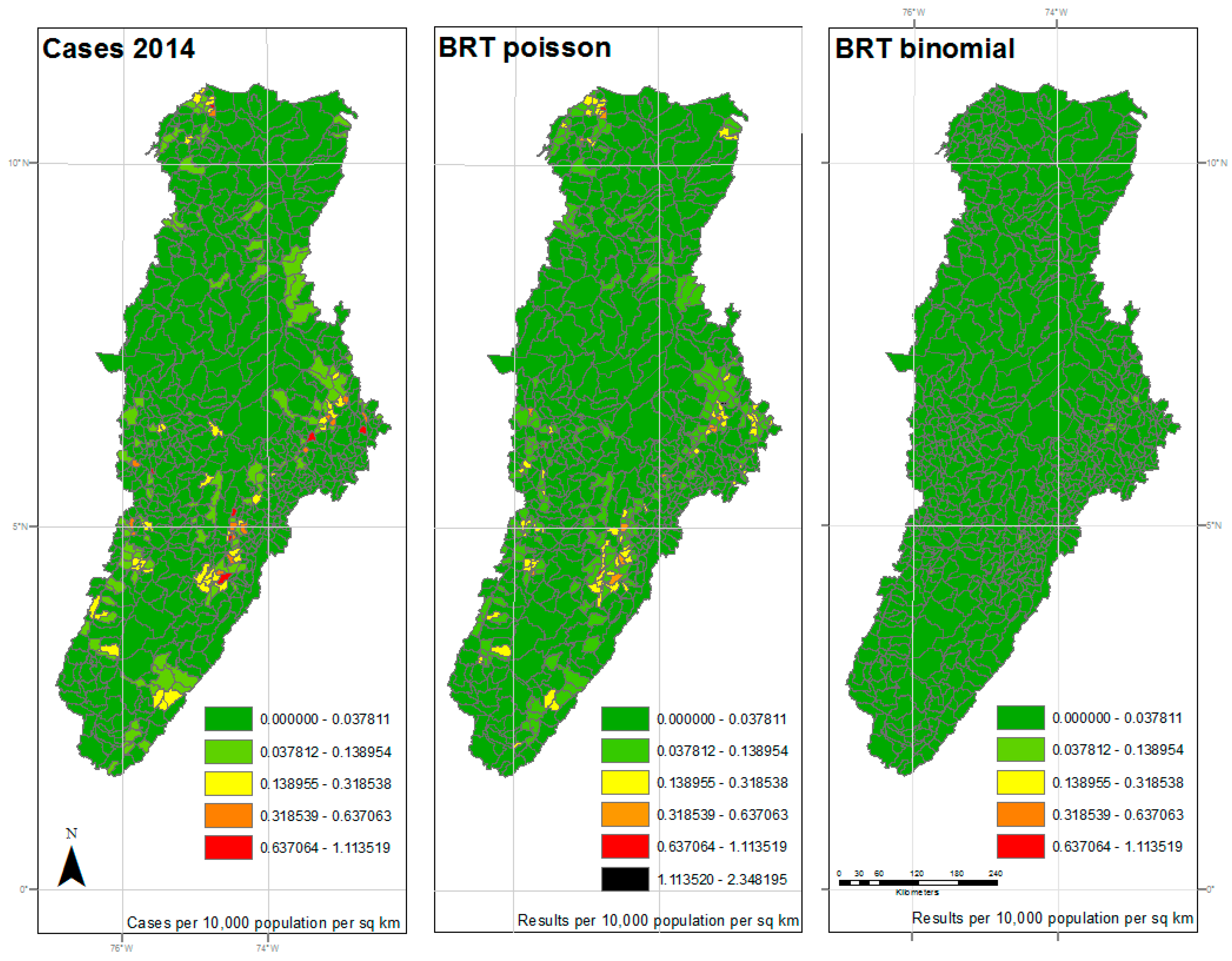
Results of 2014 analysis—The left panel represents the reported cases per 10,000 population per square kilometer for each municipality. The center panel represents the results of the BRT analysis using the Poisson family, while the right panel represents the results of the BRT analysis using the Bernoulli family. The dark green color represents very low ratios of DF, and red color reflects a higher incidence of DF. All maps used the natural breaks classification set to five classes for comparison.
Figure 4.
Results of 2014 analysis—The left panel represents the reported cases per 10,000 population per square kilometer for each municipality. The center panel represents the results of the BRT analysis using the Poisson family, while the right panel represents the results of the BRT analysis using the Bernoulli family. The dark green color represents very low ratios of DF, and red color reflects a higher incidence of DF. All maps used the natural breaks classification set to five classes for comparison.

Table 1.
Comparison of RMSE, correlation, and p-values for the Poisson and Bernoulli family models by year.
Table 1.
Comparison of RMSE, correlation, and p-values for the Poisson and Bernoulli family models by year.
| Year | Poisson | Bernoulli | ||||
|---|---|---|---|---|---|---|
| RMSE | Pearson r | p-Value | RMSE | Pearson r | p-Value | |
| 2012 | 18.013 | 0.956 | <0.001 | 62.703 | 0.298 | <0.001 |
| 2013 | 31.535 | 0.979 | <0.001 | 152.992 | 0.202 | <0.001 |
| 2014 | 35.253 | 0.986 | <0.001 | 80.500 | 0.278 | <0.001 |
Table 2.
Relative importance variables by year 1.
| Poisson Model | Bernoulli Model | ||||
|---|---|---|---|---|---|
| 2012 | 2013 | 2014 | 2012 | 2013 | 2014 |
| LD3B (52.45%) | POP_DEN (56.57%) | POP_DEN (60.22%) | POP_DEN (16.01%) | LD1B (12.67%) | LD1B (27.26%) |
| LD2B (16.42%) | LD3B (14.7%) | LD1B (11.09%) | EL3 (12.56%) | EL3 (11.46%) | LN1B (11.3%) |
| LD1B (8.28%) | UR3 (13.86%) | UR3 (8.71%) | LN3B (8.26%) | VE2B (6.63%) | POP_DEN (9.28%) |
| POP_DEN (5.97%) | LD1B (11.91%) | LD3B (3.97%) | LN3C (6.14%) | POP_DEN (6.61%) | LN2C (5.41%) |
| VE1A (4.15%) | LN1B (0.4%) | LD1A (1.96%) | LD2B (4.63%) | LN1B (5.68%) | LN1C (4.92%) |
| LD1A (2.67%) | FO3 (0.34%) | LN1A (1.83%) | LN2C (4.03%) | SA3 (4.64%) | VE2A (4.75%) |
| FO3 (1.49%) | LN1A (0.31%) | FO3 (1.61%) | LD1B (4.02%) | PR4A (4.54%) | SA3 (4.69%) |
| UR3 (1.39%) | LD2B (0.29%) | VE2A (1.47%) | UR3 (3.87%) | LN1A (4.46%) | EL3 (4.12%) |
| LN3B (1.05%) | VE2A (0.27%) | LN2C (1.33%) | LD1A (3.78%) | LD3B (4.21%) | LD1A (3.88%) |
| LN1B (1.03%) | VE2B (0.23%) | LD2B (1.33%) | VE1A (3.61%) | LN1C (4%) | PR4A (3.48%) |
| VE1B (0.87%) | LD1A (0.22%) | LN3B (1.27%) | FO3 (3.17%) | VE2C (3.99%) | LN3B (3.44%) |
| VE3B (0.84%) | VE2C (0.2%) | VE2C (0.9%) | LN1C (3.09%) | FO3 (3.82%) | FO3 (2.8%) |
| VE3A (0.77%) | LN3B (0.19%) | LN1B (0.84%) | LD3B (3.04%) | LN3B (3.76%) | UR3 (2.69%) |
| VE1C (0.7%) | LN1C (0.12%) | EL3 (0.79%) | PR4A (2.99%) | LD2B (3.68%) | VE2B (2.53%) |
| EL3 (0.42%) | EL3 (0.09%) | VE2B (0.66%) | LN1B (2.86%) | LN2C (3.65%) | LN3C (2.14%) |
| SA3 (0.35%) | SA3 (0.08%) | PR4A (0.55%) | EL1 (2.79%) | UR3 (3.37%) | LD3B (1.72%) |
| LN1A (0.35%) | LN2C (0.07%) | LN1C (0.53%) | VE3A (2.77%) | VE2A (3.29%) | VE2C (1.64%) |
| LN1C (0.28%) | EL1 (0.06%) | EL1 (0.51%) | SA3 (2.39%) | LD1A (3.26%) | LN1A (1.54%) |
| EL1 (0.22%) | PR4A (0.04%) | LN3C (0.25%) | VE3B (2.32%) | LN3C (3.2%) | EL1 (1.39%) |
| PR4A (0.12%) | LN3C (0.04%) | SA3 (0.2%) | VE3C (2.23%) | EL1 (3.08%) | LD2B (1.02%) |
1 All variables, along with their codes, are listed in the appendix.
© 2017 by the authors. Licensee MDPI, Basel, Switzerland. This article is an open access article distributed under the terms and conditions of the Creative Commons Attribution (CC BY) license (http://creativecommons.org/licenses/by/4.0/).
Share and Cite
MDPI and ACS Style
Ashby, J.; Moreno-Madriñán, M.J.; Yiannoutsos, C.T.; Stanforth, A. Niche Modeling of Dengue Fever Using Remotely Sensed Environmental Factors and Boosted Regression Trees. Remote Sens. 2017, 9, 328. https://doi.org/10.3390/rs9040328
AMA Style
Ashby J, Moreno-Madriñán MJ, Yiannoutsos CT, Stanforth A. Niche Modeling of Dengue Fever Using Remotely Sensed Environmental Factors and Boosted Regression Trees. Remote Sensing. 2017; 9(4):328. https://doi.org/10.3390/rs9040328
Chicago/Turabian StyleAshby, Jeffrey, Max J. Moreno-Madriñán, Constantin T. Yiannoutsos, and Austin Stanforth. 2017. "Niche Modeling of Dengue Fever Using Remotely Sensed Environmental Factors and Boosted Regression Trees" Remote Sensing 9, no. 4: 328. https://doi.org/10.3390/rs9040328
Note that from the first issue of 2016, this journal uses article numbers instead of page numbers. See further details here.