Fusing Observational, Satellite Remote Sensing and Air Quality Model Simulated Data to Estimate Spatiotemporal Variations of PM_2.5 Exposure in China

Abstract

Estimating ground surface PM_2.5 with fine spatiotemporal resolution is a critical technique for exposure assessments in epidemiological studies of its health risks. Previous studies have utilized monitoring, satellite remote sensing or air quality modeling data to evaluate the spatiotemporal variations of PM_2.5 concentrations, but such studies rarely combined these data simultaneously. Through assembling techniques, including linear mixed effect regressions with a spatial-varying coefficient, a maximum likelihood estimator and the spatiotemporal Kriging together, we develop a three-stage model to fuse PM_2.5 monitoring data, satellite-derived aerosol optical depth (AOD) and community multi-scale air quality (CMAQ) simulations together and apply it to estimate daily PM_2.5 at a spatial resolution of 0.1° over China. Performance of the three-stage model is evaluated using a cross-validation (CV) method step by step. CV results show that the finally fused estimator of PM_2.5 is in good agreement with the observational data (RMSE = 23.0 μg/m³ and R² = 0.72) and outperforms either AOD-derived PM_2.5 (R² = 0.62) or CMAQ simulations (R² = 0.51). According to step-specific CVs, in data fusion, AOD-derived PM_2.5 plays a key role to reduce mean bias, whereas CMAQ provides spatiotemporally complete predictions, which avoids sampling bias caused by non-random incompleteness in satellite-derived AOD. Our fused products are more capable than either CMAQ simulations or AOD-based estimates in characterizing the polluting procedure during haze episodes and thus can support both chronic and acute exposure assessments of ambient PM_2.5. Based on the products, averaged concentration of annual exposure to PM_2.5 was 55.7 μg/m³, while averaged count of polluted days (PM_2.5 > 75 μg/m³) was 81 across China during 2014. Fused estimates will be publicly available for future health-related studies.

1. Introduction

Many epidemiological studies have associated particulate matter with an aerodynamic diameter of ≤2.5 µm (PM_2.5) with adverse health outcomes, including cardiovascular and respiratory diseases [1,2], infant birth defects [3,4,5], DNA damages [6,7], cancer mortality [8,9] and many others. Severe PM_2.5 pollution in China has attracted considerable public attention [10,11,12] and inspired numerous epidemiological studies to investigate the health effects of air pollution in China since 2013 [13,14,15,16,17,18]. Accurately assessing PM_2.5 exposure is critical for estimating its health risks in such epidemiological studies. However, due to the limited number of ground monitors in China, previous studies generally ignored the spatial variation of PM_2.5 and assessed the ambient exposure uniformly using one monitor or averages of several monitors located within a city or a municipality [13,14,15,16], which causes exposure misclassification. Therefore, accurately estimating the fine-scale spatiotemporal variation of ground PM_2.5 may lay a foundation for future health-related studies of PM_2.5 in China.

Three types of numerical values have been applied in exposure assessments of ambient particles: (1) monitoring observations; (2) satellite remote sensing measurements of aerosol; and (3) air quality model simulations. Routine monitors were widely used to predict air pollution concentrations across an area using geostatistical methods such as Kriging [19,20] or land use regression (LUR) to incorporate external spatial covariates [21,22], but such monitors may be sparsely distributed in sub-urban or rural areas. The PM_2.5 monitoring network has been rapidly spreading over China. In 2013, only approximately 70 cities or municipalities were covered by official sites of the China Environmental Monitoring Center (CEMC), whereas by 2015, the number had increased to approximately 330. However, monitoring data remain inadequate for characterizing the national-scale spatial variability of PM_2.5 in China.

The satellite remote sensing technique can retrieve integrated column concentrations of gases and aerosol from the bottom to top of the atmosphere and has been applied to assess ground surface air pollution [23]. Satellite-derived aerosol optical depth (AOD) has been successfully associated with ground PM_2.5 [24] and has thus been used to generate spatiotemporal estimators of PM_2.5 by acting as a primary predictor in statistical models such as LUR [25,26,27] or being calibrated by ratios (PM_2.5/AOD) simulated by a chemical transport model (e.g., GEOS-Chem) [28,29]. However, due to meteorological or geographical conditions, non-randomly missing values in satellite-derived AOD caused absent estimates of PM_2.5 in specific periods (e.g., winter [26]) or areas (e.g., deserts [28]).

Air quality models, such as the community multi-scale air quality model (CMAQ), simulate pollution concentrations based on emission inventories and chemical and physical processes driven by a meteorological model, such as the weather research and forecasting model (WRF) [30], and can provide exposure estimates with spatiotemporally complete coverage [31,32]. However, the accuracy of air quality models depends on the uncertainty of emission inventories and meteorological inputs and has thus been reported to vary with seasons and locations [33].

Hybrid models have been developed to combine different numerical values of air pollutants to improve exposure estimates. Beckerman et al. [34] estimated monthly PM_2.5 on an 8.9 km × 8.9 km grid over the contiguous United States (US) through combining LUR of monitors and satellite PM_2.5 derived from GEOS-Chem and AOD. Mcmillan et al. [35] developed a hierarchical Bayesian spatiotemporal model to bring monitors and CMAQ together and generated daily PM_2.5 and O₃ on both 36 km × 36 km and 12 km × 12 km grids over the US. Friberg et al. [36] introduced a method to fuse CMAQ simulations and monitoring observations for daily estimates of multiple air pollutants on a 12 km × 12 km grid over Georgia, US. Liu et al. [18] utilized the Ensemble Kalman Filter (EnKF) to assemble in situ observations with daily stimulations of PM_2.5 from an air quality model across China, and applied the analyzed products in risk assessment of chronic exposure to ambient pollution. Beloconi et al. [27] mixed spatiotemporal Kriging maps of monitoring data and satellite AOD to estimate fine-scale (1 km × 1 km) daily estimates of PM_2.5 and PM₁₀ during 2002–2012 over London.

To further increase the accuracy of exposure assessments of PM_2.5 via making full use of available data, this study aims to develop a fused estimator to join monitoring, satellite remote sensing and air quality modeling data together. Our approach incorporated: (1) monitoring records from routine sites as reference measurements of PM_2.5; (2) CMAQ simulations as prior knowledge, which provides completely spatiotemporal coverage of PM_2.5; and (3) satellite AOD as alternative observations with wider spatial coverage than monitors and higher accuracy than CMAQ. We applied a three-stage model for the fused estimator. In Step 1, we derived ground surface PM_2.5 from satellite AOD and calibrated CMAQ simulations by monitoring data using two separate regression models. In Step 2, we combined AOD-derived PM_2.5 and calibrated-CMAQ PM_2.5 using a maximum likelihood method. In Step 3, we incorporated the spatiotemporal autocorrelation of the monitoring data in the final estimator through interpolating the residuals in Step 2. We illustrated the three-stage model by a practice to develop daily maps of PM_2.5 on a regular grid of 0.1° × 0.1 ° over China. The performance of the statistical models was assessed using cross-validation (CV) methods by steps.

2. Materials and Methods

2.1. Data Description

2.1.1. PM_2.5 Monitoring Data

We collected hourly PM_2.5 measurements from three monitoring networks in the year 2014, including the CEMC sites [37], the sites of the Beijing Municipal Environmental Monitoring Center [38] and the sites of the Guangdong Environmental Monitoring Center [39]. Duplicate monitoring sites among these three networks were removed, leaving a total of 944 sites (Figure 1). According to the Chinese National Ambient Air Quality Standard (CNAAQS, GB3095-2012) released in 2012, the ground-based PM_2.5 data are measured using the tapered element oscillating microbalance (TEOM) technique or the beta-attenuation method. For each monitor, we averaged PM_2.5 by day and excluded the dates with less than 19 hourly measurements. Figure 1 presents locations of the monitors.

2.1.2. Satellite Remote Sensing of AOD

Satellite-derived AOD data during 2014 were obtained from moderate resolution imaging spectroradiometer (MODIS), equipped on two earth observing system satellites, Terra and Aqua, which are operated by US National Aeronautics and Space Administration (NASA). Terra (Aqua) scans the earth at 10:30 a.m. (1:30 p.m.) with a global coverage of 1–2 days. They retrieved AOD from visible and near-infrared electromagnetic signals at nadir. Level 2 MODIS AOD products (collection 6) with a spatial resolution of 10 km × 10 km were collected from Atmosphere Archive and Distribution System [40]. L2 swath data were resampled into a fixed grid, which covers the whole investigated regions with a spatial resolution of 0.1° × 0.1° via area-weighted averaging. The AOD_550_Dark_Target_Deep_Blue_Combined dataset with QA Flag equal to 2 or 3 were utilized in this study. According to Ma et al. [41], we combined Terra/Aqua MODIS AOD measurements together to increase the spatial coverage of AOD measurements.

2.1.3. Satellite Remote Sensing Covariates for AOD-Derived PM_2.5

Satellite normalized difference vegetation index (NDVI) and fire spots (FS) were obtained from combined MODIS products. We aggregated monthly products of NDVI with a spatial resolution of 1 km × 1 km into seasonal averages over the regular grid of 0.1° × 0.1°. Daily counts of FS within a 75 km buffer around each centroid of the grid were calculated based on the location and time of fires, collected from MODIS burned area products. Integrated column concentrations of NO₂ were obtained from Ozone Monitoring Instrument (OMI), launched on Aura. Level 2 products of column NO₂ with a spatial resolution of 13 km × 24 km were prepared into seasonal means with a spatial resolution of 0.1° × 0.1°. The above data can be accessed from Land Process Distributed Active Archive Center [42], MODIS Active Fire and Burned Area Products [43] and Goddard Earth Sciences Data and Information Services Center [44].

2.1.4. WRF-CMAQ Simulation

In this study, the WRF model version v3.5.1 [45] and the CMAQ model version 5.1 were used to simulate the daily variations of PM_2.5 over China. The WRF model is driven by the National Centers for Environmental Prediction Final Analysis (NCEP-FNL) reanalysis data as initial and boundary conditions (ICs and BCs). Meteorological parameters simulated by WRF model were applied to drive CMAQ. Our CMAQ simulations utilized CB05 as the gas-phase mechanism, AERO6 as the aerosol module, and Regional Acid Deposition Model (RADM) as the aqueous-phase chemistry model. Boundary conditions for our CMAQ model were provided by dynamic GEOS-Chem simulation [46]. The anthropogenic emissions for Mainland China during 2014 are derived from the Multi-resolution Emission Inventory of China [47]. Detailed model configurations for WRF-CMAQ were presented in our previous study [48]. We simulated meteorological variables including ground wind speed (WS), planetary boundary layer height (PBL), ground ambient pressure (PS), and ground relative humidity (RH) by WRF and PM_2.5 by CMAQ with a spatial resolution of 36 km × 36 km, which were further downscaled to the 0.1° × 0.1° grid using an offline ordinary Kriging method [49]. The daily means of simulations were interpolated in spatial dimensions for each variable separately. The purpose of downscaling is to spatially match WRF-CMAQ simulations with the rest data. Validations for CMAQ-simulated PM_2.5 at both spatial resolutions (0.1° and 36 km) were performed using monitoring data, which are presented in Figures S2 and S3 and briefly illustrated in the Discussion Section. After downscaling, CMAQ-simulated PM_2.5 covered 100% of spatiotemporal coordinates (99,351 pixels × 365 days), while the in situ observations or AOD measurements only covered 0.54% or 31.56% of spatiotemporal coordinates, respectively.

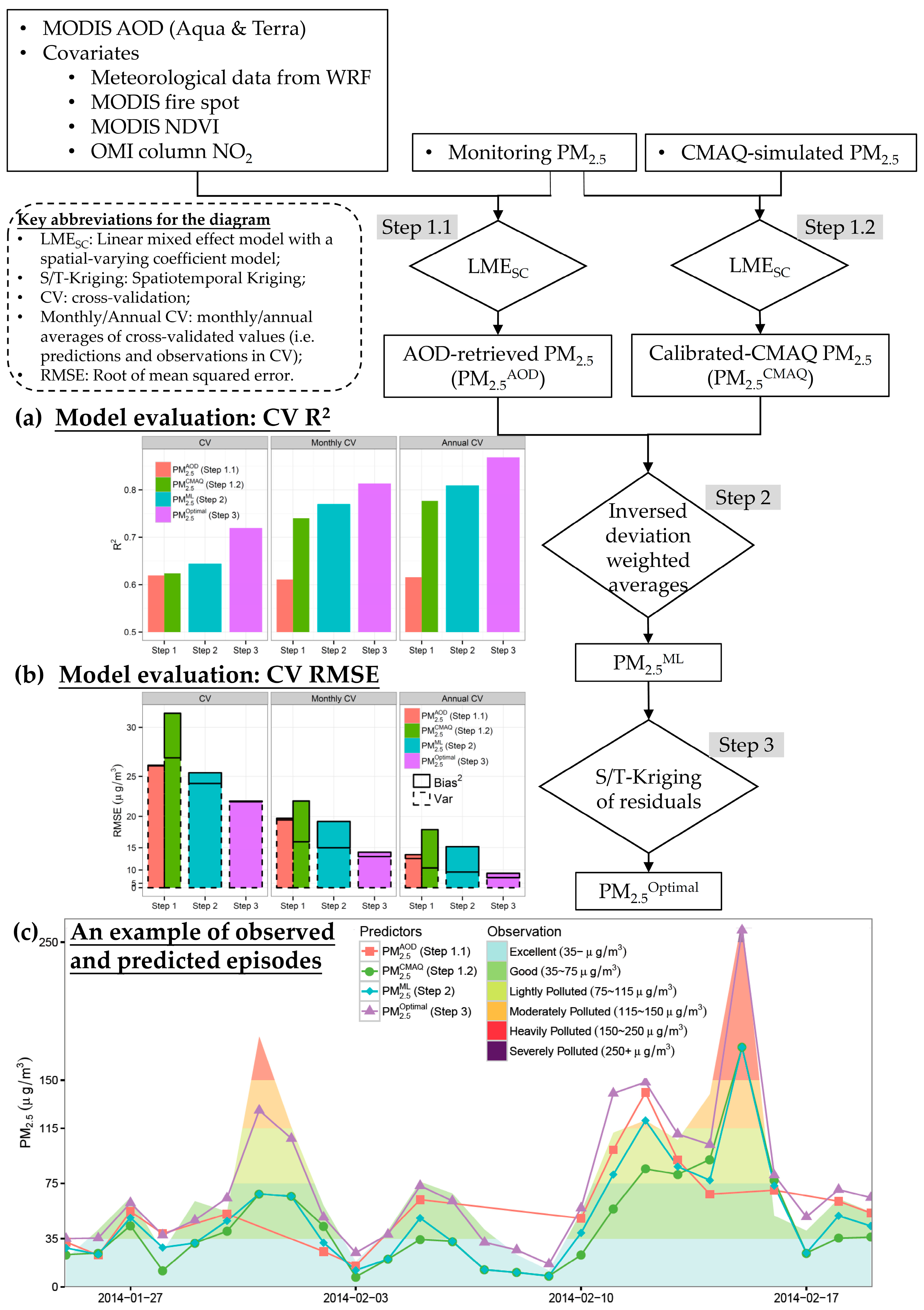
2.2. Statistical Analysis

The modeling framework of exposure assessment included three steps, which were presented in Figure 2. Briefly, we first developed two regression models (Steps 1.1 and 1.2) to associated AOD or CMAQ with in situ observations of PM_2.5, separately; then, the estimates from the two models were combined based on a maximum likelihood (Step 2); and, finally, we incorporated spatiotemporal autocorrelations of the monitoring PM_2.5 (Step 3).

2.2.1. Step 1.1: AOD-Derived PM_2.5

Based on the mature methodology developed by Ma et al. [41], we first derived PM_2.5 from satellite-retrieved AOD with the auxiliary variables, which were selected according to experimental findings (e.g., RH [50,51]) or empirical results on PM_2.5–AOD associations (e.g., NO₂ [52] and FS [26]). Instead of using the linear mixed effect model (LME) [41], we developed an updated version, a linear mixed effect model with a spatial-varying coefficient (LME_SC) model:

$$\begin{array}{ll}{\mathrm{PM}}_{2.5,\mathbf{s}\mathrm{t}}=& \mu +[{\beta }_1+f(s)]{\mathit{AOD}}_{\mathit{st}}+({\beta }_2+{\beta }_{2,j}^{\prime }){\mathit{WS}}_{\mathit{st}}+({\beta }_3+{\beta }_{3,j}^{\prime }){\mathit{PBL}}_{\mathit{st}}\\ & +({\beta }_4+{\beta }_{4,j}^{\prime }){\mathit{PS}}_{\mathit{st}}+({\beta }_5+{\beta }_{5,j}^{\prime }){\mathit{RH}}_{\mathit{st}}+({\beta }_6+{\beta }_{6,j}^{\prime }){\mathit{FS}}_{\mathit{st}}\\ & +({\beta }_7+{\beta }_{7,j}^{\prime }){\mathit{NDVI}}_{\mathit{sj}}+({\beta }_8+{\beta }_{8,j}^{\prime }){\mathit{NO}}_{2,\mathit{sj}}+{ϵ}_{\mathit{s}t},\end{array}$$

(1)

where

$$f\left(\mathit{s}\right)=b{\prime }_{1,t}{\eta }_1\left(\mathit{s}\right)+b{\prime }_{2,t}{\eta }_2\left(\mathit{s}\right)+\cdots +b{\prime }_{\mathrm{k},t}{\eta }_k\left(\mathit{s}\right),$$

$${ϵ}_{\mathit{s}t}~N\left(0,{\sigma }^2\right),$$

$$[b_{i,t=1}^{\prime },b_{i,t=2,}^{\prime }\cdots ,b_{i,t=T,}^{\prime }]\prime ~N\left(0,{\mathrm{\Phi }}_i\right),i=1,\cdots ,\mathrm{k};$$

$$[{\beta }_{i,j=1}^{\prime },{\beta }_{i,j=2,}^{\prime }{\beta }_{i,j=3}^{\prime },{\beta }_{i,j=4}^{\prime }]\prime ~N\left(0,{\mathrm{\Phi }}_i\right),i=2,\cdots ,9$$

In the LME_SC, s, t and j denote spatial coordinates (longitude and latitude at the centroid of each pixel), daily and seasonal index, respectively; ${\mathrm{PM}}_{2.5,s\mathrm{t}}$ denotes in situ observations at spatial location s and date t; and $\mu , {\beta }_1,\cdots , {\beta }_8$ denote fixed intercept and slopes for covariates including: (1) daily values of AOD, WS, PBL, PS, RH and FS; and (2) seasonal values of NDVI and ${\mathrm{NO}}_2$. $\beta {\prime }_{2,j}, \dots , \beta {\prime }_{8,j}$ denote seasonally-specific random slopes for the other covariates than AOD. $f\left(s\right)$ denotes a spatial-varying coefficient for AOD and is expanded by a given set of k-dimensional basis functions (e.g., local bisquare functions [53]) and daily-specific random slopes ($b{\prime }_{,t}$). In this study, for computing efficiency, we expanded $f\left(s\right)$ by 2-D splines provided by R package mgcv [54]. ηs became known values depended on spatial coordinates (s), once the specific form of basis functions was determined. Thus, the inference of coefficients ($b{\prime }_{\cdot ,t}$) in $f\left(\mathit{s}\right)$ was done in regression procedure, simultaneously with other parameters (e.g., βs) in Equation (1). If $f\left(\mathit{s}\right)$ is simplified as a one-dimensional daily-specific random slope ($\beta {\prime }_{1,t}$), the LME_SC will be reduced to a LME, which has been utilized in previous studies to generate AOD-derived PM_2.5 [41]. LME method has disadvantages in generating spatially smoothing predictors, especially near the provincial boundaries. Through introducing spatial-varying coefficients, LME_SC fixed this problem and was evidenced to outperform LME by our cross-validation results. Detailed comparisons are presented in the Discussion Section. Spatial and temporal patterns for PM_2.5–AOD associations (${\beta }_1+f\left(s\right)$) are presented in Figure S8. Fitted value and its standard deviation (SD) from Equation (1) are denoted by PM_2.5^AOD and SD^AOD, respectively. We named PM_2.5^AOD as “AOD-derived PM_2.5” in this study. Equation (1) was fitted based on 92,644 in situ observations collocated with AOD data, and PM_2.5^AOD was estimated at all spatiotemporal coordinates, where AOD existed.

2.2.2. Step 1.2: Calibrated-CMAQ PM_2.5

We calibrated CMAQ simulated PM_2.5 with the in situ observations by a similar LME_SC model:

$${\mathrm{PM}}_{2.5,s\mathrm{t}}={\mu }^{*}+\left[{\beta }_1^{*}+f^{*}\left(s\right)\right]{\mathrm{CMAQ}}_{s\mathrm{t}}+{ϵ}_{\mathit{s}t}$$

(2)

where ${\mathrm{CMAQ}}_{s\mathrm{t}}$ denotes downscaled CMAQ-simulated PM_2.5 with a spatial resolution of 0.1° × 0.1°. In Equation (2), we utilized original scale instead of log-scale of PM_2.5 in order to guarantee comparable error terms (${ϵ}_{\mathit{s}t}$) to that in Equation (1), although logarithm transform was usually used to reduce the bias caused by violation of normality assumption of PM_2.5 in the regression analysis. Spatial and temporal variations of estimated coefficients of CMAQ-simulated PM_2.5 (${\beta }_1^{*}+f^{*}\left(s\right)$) are presented in Figure S9. Fitted value and its SD from Equation (2) are denoted by PM_2.5^CMAQ and SD^CMAQ, respectively. We named PM_2.5^CMAQ as “calibrated-CMAQ PM_2.5” in this study. Equation (2) was fitted based on all 294,122 in situ observations collocated with CMAQ data, and PM_2.5^CMAQ was estimated at all spatiotemporal coordinates.

2.2.3. Step 2: Inversed Deviation Weighted Averages

To minimize the uncertainty, we derived a maximum likelihood estimator (PM_2.5^ML) for the collocated AOD-derived PM_2.5 and calibrated-CMAQ PM_2.5. Assuming the normality for the fitted values (PM_2.5^AOD and PM_2.5^CMAQ), the maximum likelihood estimator can be simplified as inversed deviation weighted averages, shown as follows:

$${\mathrm{PM}}_{2.5,s\mathrm{t}}^{\mathrm{ML}}=\frac{{\mathrm{PM}}_{2.5,\mathrm{st}}^{\mathrm{AOD}}/{({\mathrm{SD}}_{s\mathrm{t}}^{\mathrm{AOD}})}^2+{\mathrm{PM}}_{2.5,\mathrm{st}}^{\mathrm{C}}/{\left({\mathrm{SD}}_{s\mathrm{t}}^{\mathrm{CMAQ}}\right)}^2}{1/{\left({\mathrm{SD}}_{s\mathrm{t}}^{\mathrm{ML}}\right)}^2}$$

(3)

where

$${({\mathrm{SD}}_{s\mathrm{t}}^{\mathrm{ML}})}^2=\frac{1}{1/{({\mathrm{SD}}_{s\mathrm{t}}^{\mathrm{AOD}})}^2+1/{\left({\mathrm{SD}}_{s\mathrm{t}}^{\mathrm{CMAQ}}\right)}^2}$$

For the places where the AOD is missing, the PM_2.5^ML is defined identically as PM_2.5^CMAQ.

2.2.4. Step 3: Spatiotemporal Kriging of the Residuals

Taking spatiotemporal autocorrelation of PM_2.5 into consideration, we interpolated the residuals (${\mathrm{e}}_{s\mathrm{t}}={\mathrm{PM}}_{2.5,s\mathrm{t}}-{\mathrm{PM}}_{2.5,s\mathrm{t}}^{\mathrm{ML}}$) using spatiotemporal Kriging (S/T-Kriging) based on a product-sum covariance function [55]. Assuming a stationary multivariate normal distribution for the residuals (${\mathrm{e}}_{s\mathrm{t}}$), the variance–covariance matrix can be captured by a function (C) of the spatiotemporal coordinates, as shown in follows:

$$\left[{\mathrm{e}}_{s\mathrm{t}}\right]\equiv E\sim MVN\left(0,\Sigma \right),$$

$$Cov\left({\mathrm{e}}_{s_{\mathrm{i}}{\mathrm{t}}_{\mathrm{i}}},{\mathrm{e}}_{s_{\mathrm{j}}{\mathrm{t}}_{\mathrm{j}}}\right)\equiv {\Sigma }_{\mathrm{i},\mathrm{j}}=\mathrm{C}\left({||{\mathit{s}}_i-{\mathit{s}}_j||}_2,{||t_i-t_j||}_1 |\mathbf{\theta }\right),$$

where $\mathbf{\theta }$ denotes the tuning parameters in the covariance function (C) and can be estimated using variogram approach. For a spatiotemporal point (s*, t*), where in situ observation of PM_2.5 does not exist, the residual can be interpolated as ${\hat{\mathrm{e}}}_{s^{*}{\mathrm{t}}^{*}}=Cov\left({\mathrm{e}}_{s^{*}{\mathrm{t}}^{*}},E\right){\Sigma }^{-1}E$. Therefore, the optimal estimates of PM_2.5 can be derived as

$${\mathrm{PM}}_{2.5,s\mathrm{t}}^{\mathrm{Optimal}}={\mathrm{PM}}_{2.5,s\mathrm{t}}^{\mathrm{ML}}+{\hat{\mathrm{e}}}_{s\mathrm{t}}$$

(4)

For more details of S/T-Kriging, please refer to Chapter 6 in Cressie and Wikle [55].

2.3. Model Evaluation

Previous studies usually evaluated statistical performance of PM_2.5 estimators by the 10-fold cross validation (CV₁₀), which randomly divides the monitoring data into ten folds and iteratively leaves one fold out as the testing dataset to assess the predictions from a model trained by the remaining data. For independent data, the root of mean squared error (RMSE) has been considered an unbiased estimator for prediction accuracy [56]. However, for spatiotemporally auto-correlated PM_2.5 data, CV₁₀ may underestimate prediction errors [57]. To fairly evaluate the models, we designed isolated-site cross-validation (CV_IS), in which we held out about 10% of the monitoring sties and used all measurements from the testing sites to validate the modeling results based on the rest data. The testing sites were randomly selected with two constraints: (1) they should be separated from the training sites by more than 25 km; and (2) they should be universally spanned over the study domain, especially areas with dense population. In this study, we involved 91 testing sites with a minimum distance from the remained sites of 26.2 km, as shown in Figure 1. The testing set contained 27,800 samples out of 294,122 total daily values of monitoring measurements. We kept multiple testing values located within one grid at the same time point, because the discrepancy among those values represents the error caused by spatially aggregation, which should not be ignored in model evaluation. A comparison between CV₁₀ and CV_IS was performed based on AOD-derived PM_2.5 from a LME model (Figure S1), and more detailed rationale of CV_IS is presented in the Discussion Section. We also evaluated the three-stage model using the same CV_IS data step by step. The CV_IS analysis of the intermediate estimators illustrated how the errors propagate in our data fusion model.

3. Results

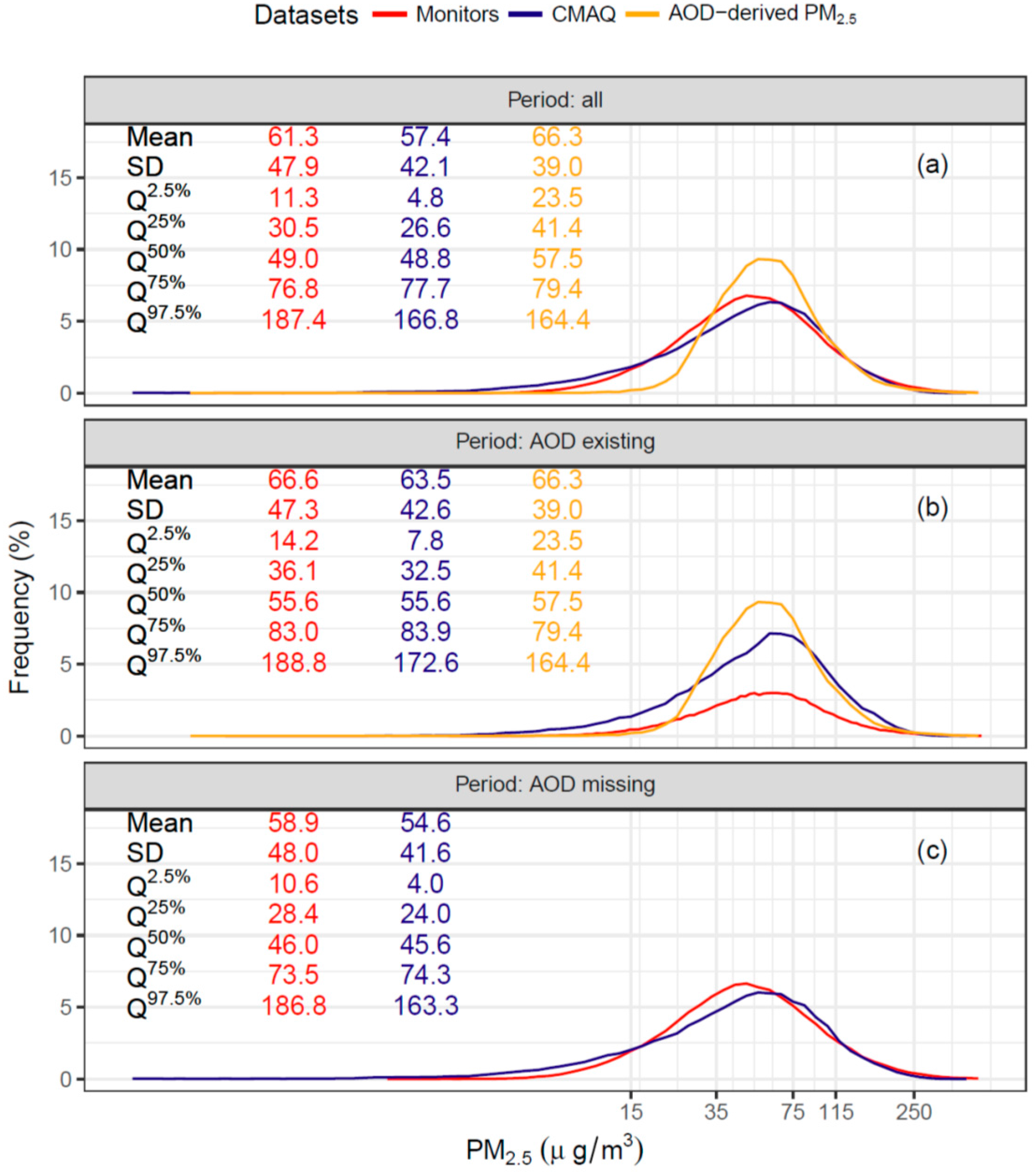
3.1. Descriptive Statistics for Inputs of Data Fusion

Figure 3 presents the frequency distributions and summary statistics of in situ observations, CMAQ simulations and AOD-derived estimates of PM_2.5. CMAQ simulated or AOD-derived PM_2.5 concentrations were extracted at the same spatiotemporal coordinates of monitoring data, in order to compare the three types of inputs in our model. During 2014, the overall mean of the monitoring PM_2.5 is 61.3 μg/m³, which is slightly higher that of CMAQ-simulated PM_2.5 (57.4 μg/m³) but lower than that of AOD-derived PM_2.5 (66.4 μg/m³), which suggests systematic bias in the latter two datasets. However, after excluding the observational PM_2.5 at the time points, when AOD is missing, the mean of monitoring data is increased to 66.6 μg/m³ (Figure 3b), which is close to that of AOD-derived PM_2.5. A Kolmogorov–Smirnov test indicated that monitoring data presented significantly different distributions depended on the missing status of AOD. According to our findings, in China AOD incompleteness occurred non-randomly and was influenced by the ambient concentrations of PM_2.5, which leads to sampling errors in AOD-derived PM_2.5. The systemic bias between frequency distribution of AOD-derived PM_2.5 and that of overall monitoring data was partially caused by the sampling errors of satellite-derived AOD.

3.2. Cross-Validation Results for the Estimates of the Three-Stage Model

Figure 4a presents the CV_IS results of the three-stage model. The final estimator of the model (PM_2.5^Optimal) is in good agreement with the observational data (R² = 0.72). The root of mean squared error (RMSE) is 23.0 μg/m³, which accounts for 55% of the SD of observational PM_2.5 (defined as normalized root of mean squared error (NRMSE)) and 41% of the mean of observational PM_2.5 (defined as relative prediction error (RPE)). The mean bias is 4.9 μg/m³, which suggests that PM_2.5^Optimal underestimate the true values. The slope of a linear regression of the predictors against the observations is 0.76, lower than 1, which indicates that PM_2.5^Optimal may be over-smoothed. Among 27,800 testing observations in CV_IS, collocated satellite-derived AOD data are available for 9530 of them. In other words, at one third of the CV points, PM_2.5^Optimal were estimated based on AOD, CMAQ and ground monitors, while at the other CV points, PM_2.5^Optimal were estimated based on the latter two. To evaluate the capacity of PM_2.5^Optimal to assess the long-term exposure to ambient PM_2.5, we averaged both the predicted and the observed values in CV_IS by month or by year (Figure 4a). Because averaging can lower the variance of predictors, the CV_IS R², respectively, increases to 0.81 or 0.87 for monthly or annually averages, which indicates that PM_2.5^Optimal may be more appropriate to study chronic exposure than acute exposure to PM_2.5.

CV_IS results for the intermediate estimators (i.e., PM_2.5^AOD, PM_2.5^CMAQ and PM_2.5^ML) of the three-stage model are shown in Figure 2 and Figure 4b-d. Generally speaking, the predicting errors were decreased step by step in our modeling process. For example, in daily scale, CV_IS R² increases from 0.62 for either PM_2.5^AOD or PM_2.5^CMAQ in Step 1, to 0.64 for PM_2.5^ML in Step 2 and further to 0.72 for PM_2.5^Optimal in Step 3. The decreasing trend in CV_IS RSME is mostly dominated by the shrinkage in variations of predicting errors due to aggregations of multiple predictors at each testing site. As the more biased estimator, PM_2.5^CMAQ is mixed with the less biased estimator, PM_2.5^AOD, in data fusion, biasness of the combined estimators (PM_2.5^ML and PM_2.5^Optimal) lays between the former two. Although PM_2.5^AOD is less biased than the others; it may fail to capture some PM_2.5 episodes due to incompleteness of satellite data (Figure 2c). Such weaknesses are partially overcome by data fusion (Figure 2c). The detailed CV_IS scatterplots for the intermediate estimators are presented in the Figure 4b–d.

We also explored temporal (Figure S6) and spatial (Figure S7) variations of CV_IS results. To evaluate the temporal variation of CV_IS errors, we calculated the statistics, including R², RMSE and NRMSE by dates. The daily CV_IS results reflected the final estimator’s capacity to capture spatial variations of PM_2.5. The CV_IS RMSE for PM_2.5^Optimal is proportional to the observed value and thus was varied seasonally (higher in colder season, but lower in warmer season). However, we found significant trend neither in daily NRMSEs nor in daily R²s (Figure S6), which indicates that the accuracy of PM_2.5^Optimal is temporally constant. Analogously, we also calculated CV_IS statistics by sites to evaluate the final estimator’s capacity to capture temporal variations of PM_2.5. CV_IS results by sites displayed significantly spatial patterns, which indicates that PM_2.5^Optimal is more accurate in eastern China, but less in western China (Figure S7). Partial reason is that the accuracy of PM_2.5^Optimal tends to increase with the density of training sites (Figure 5), which are more clustered in eastern China, especially the urban areas (e.g., Yangtze River Delta or Pearl River Delta metropolitan region).

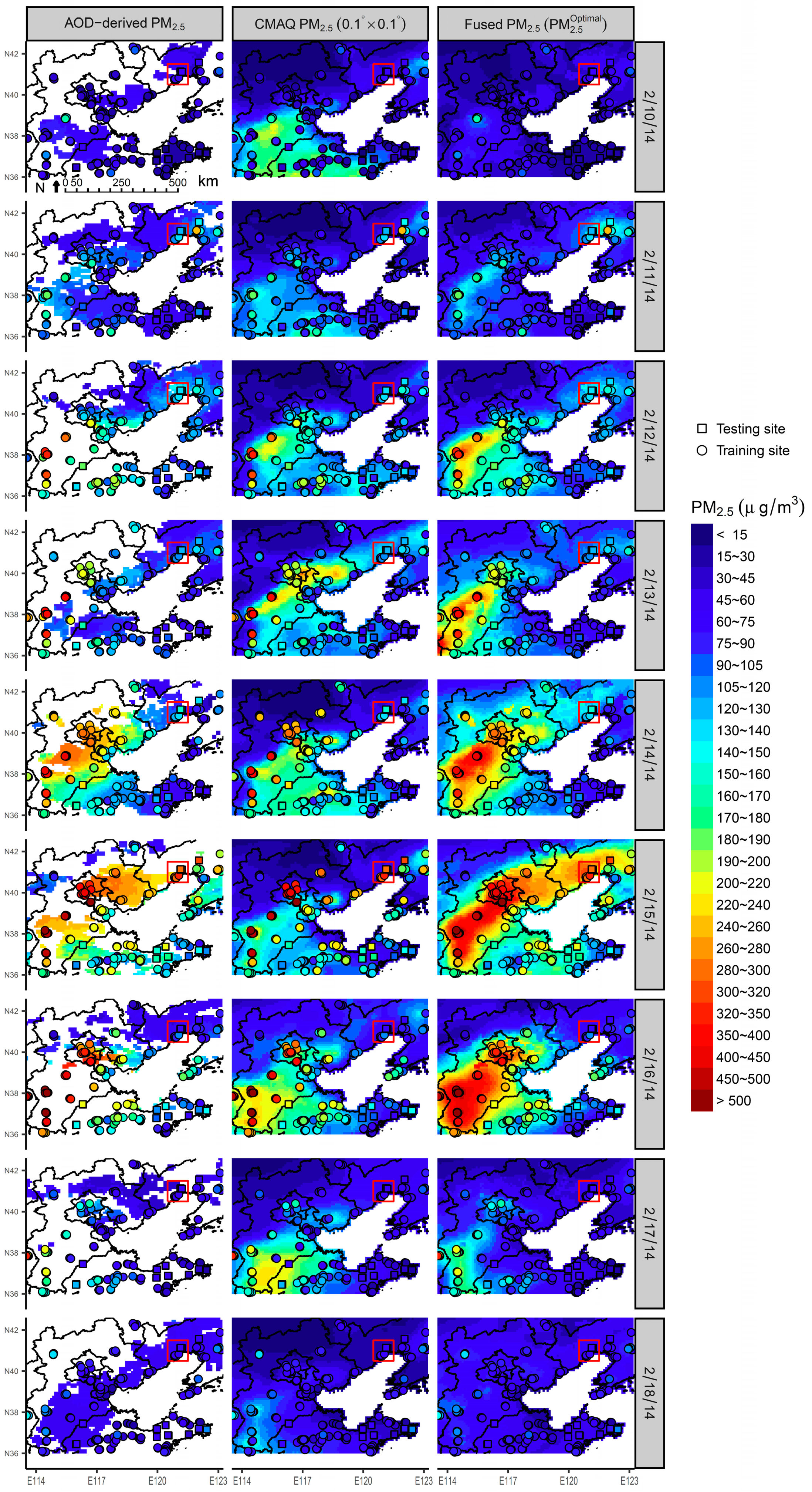
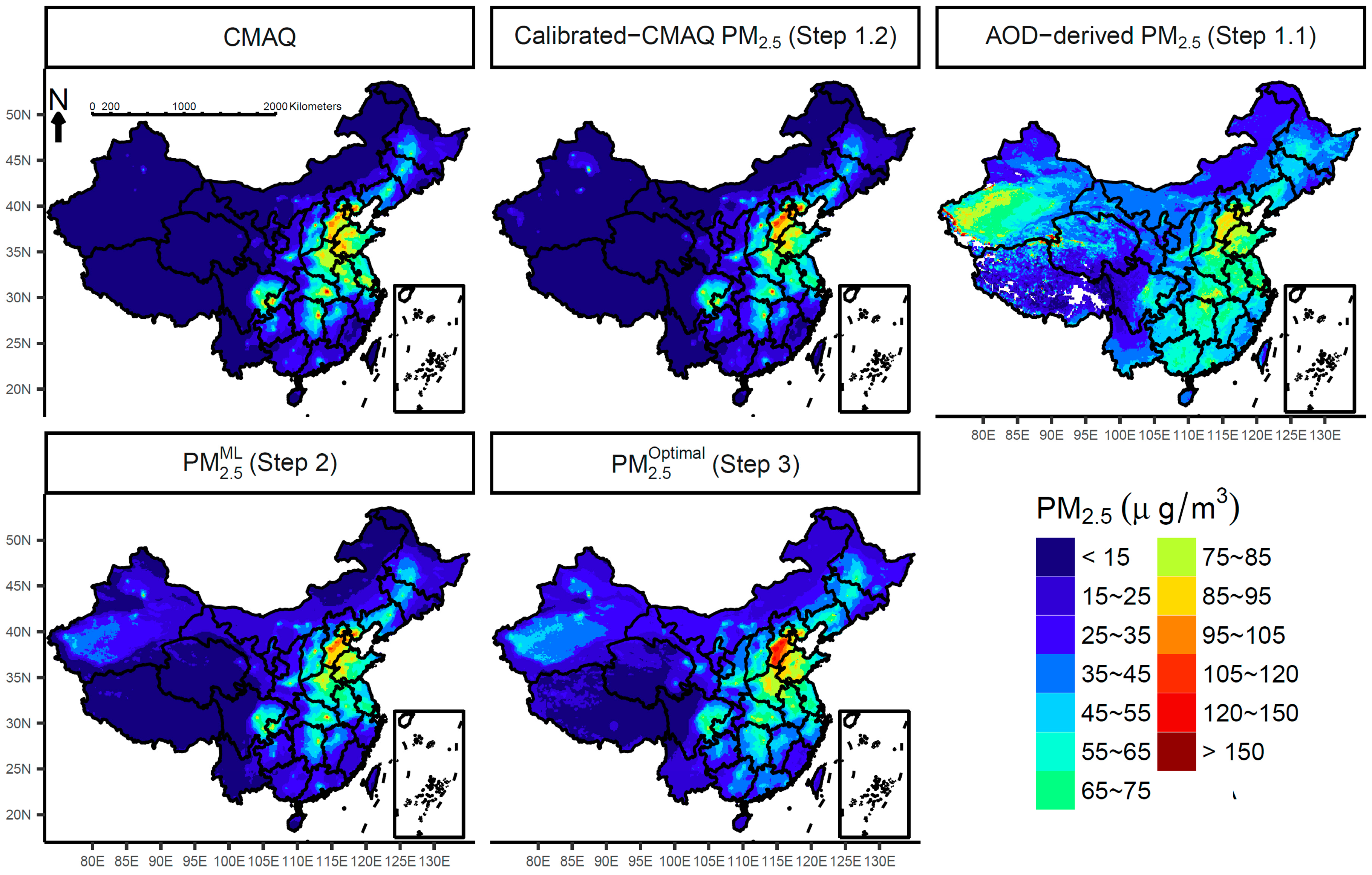
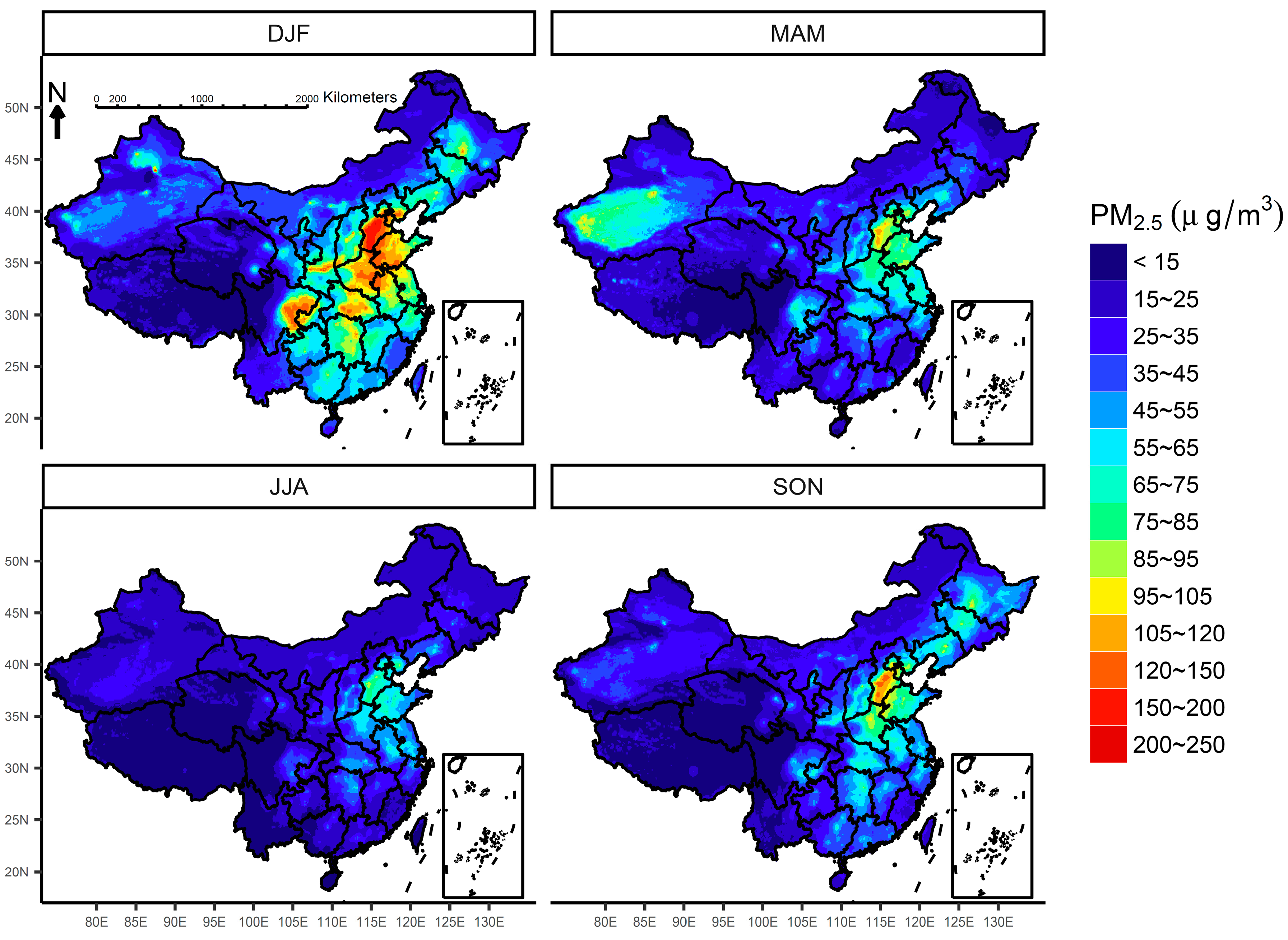
3.3. The Fitted Spatial and Seasonal Patterns of PM_2.5 in China

Figure 6 presents the annual maps of PM_2.5 fitted by the three-stage model and its intermediate steps. Different methods displayed consistent patterns in spatial variation of PM_2.5, particularly across eastern China, where PM_2.5 pollutants were dominated by anthropogenic sources. During 2014, the hot-spots of PM_2.5 (PM_2.5^Optimal = 85~120 μg/m³) spanned over North China Plain (the municipalities of Beijing and Tianjin, and the provinces of Hebei, Henan and Shandong). The moderately polluted areas (PM_2.5^Optimal = 45~85 μg/m³) occupied Sichuan Basin (Sichuan Province and Chongqing Municipality), Loess Plateau (Shanxi Province and middle of Shaanxi Province), Yangtze Plain (Shanghai Municipality, the provinces of Anhui, Jiangsu, Hunan and Hubei) and Northeast China Plain (the provinces of Heilongjiang, Liaoning and Jilin). The major divergence among these maps exists in the deserted areas of northwestern China. CMAQ-based estimators (i.e., CMAQ-simulated PM_2.5 and calibrated-CMAQ PM_2.5) failed to capture PM_2.5 from natural sources and underestimated the concentrations across the Taklamakan desert. In the fused estimators (i.e., PM_2.5^ML and PM_2.5^Optimal), the problem was fixed by introducing AOD data. Figure 7 presents seasonal maps of PM_2.5 fitted by PM_2.5^Optimal, which confirms that PM_2.5 concentrations are higher during winter (DJF) and autumn (SON), but lower in summer (JJA) and spring (MAM). The sever pollution of PM_2.5 in colder seasons might be attributed by fossil fuel combustions, especially across northern China. Seasonal maps for the other estimators are presented in supplemental Figure S4.

3.4. Exposure Assessments Based on the Fused Estimates

The fused estimator of PM_2.5 (PM_2.5^Optimal) will support exposure assessments in future health-related studies. AOD or CMAQ based estimator of PM_2.5 has been utilized to study long-term rather than short-term exposure to ambient pollution [18,58], because of data availability or data accuracy on daily scale. For example, we visualized spatiotemporal distributions of CMAQ simulations and AOD-derived PM_2.5 with the corresponding monitoring data during an episode of haze around Beijing-Tianjin-Hebei region in Figure 8. According to the maps, AOD-based method overlooked some hotspots due to incompleteness and could not capture the whole polluting procedure; whereas CMAQ simulations underestimated the severity of haze due to systematic errors. Unlike them, the fused estimates accurately characterized the growth, expansion and elimination of the haze. Therefore, PM_2.5^Optimal can serves as exposure estimates to study either acute or chronic effects of PM_2.5. For example, combining PM_2.5^Optimal with county-level data of China’s sixth census, we assessed both annual and daily exposures to PM_2.5 across China in 2014. Accordingly, population-weighted concentration of annual exposure to ambient PM_2.5 was 55.7 μg/m³ and 82% of total population inhabited in the places exceeding WHO Air Quality Interim Target-1 (35 μg/m³), whereas population-weighted count of polluted and heavily-polluted days (defined as daily mean of PM_2.5 > 75 μg/m³ or 150 μg/m³ by CNAAQS) was 81 and 14 days, respectively.

4. Discussion

In this paper, we developed a three-stage model to estimate spatiotemporal variations of PM_2.5 through fusing CMAQ simulations, satellite remote sensing measurements and ground monitoring data together. We illustrated the method by a practice to generate daily PM_2.5 maps with a spatial resolution of 0.1° × 0.1° across China during 2014. The CV results evidenced that the fused estimator (PM_2.5^Optimal) was in good agreement with the observational PM_2.5, and outperformed the estimators based on either AOD or CMAQ data alone.

AOD-based methods have been widely utilized to estimate PM_2.5 concentrations on regional [52], national [41] or global scale [29]. Among them, LME or its extension has been more widely used because of computing efficiency. For example, in China, Ma et al. [41] developed high-quality estimates of PM_2.5 covering a long-period from 2004 to 2013, through joining a LME and a generalized additive model (GAM) to retrieve PM_2.5 from MODIS AOD at 0.1° resolution; and tested their estimates by a CV₁₀ of monitoring data in 2013 (RMSE = 27.99 μg/m³, R² = 0.78 and RPE = 36.3% for the first-stage estimator from LME; RMSE = 27.42 μg/m³, R² = 0.79 and RPE = 35.6% for the final estimator from LME + GAM). In this paper, we fitted a similar LME model through reducing the spatial-varying coefficient ($f\left(s\right)$) in Equation (1) to a one-dimensional random slope; and evaluated it by CV₁₀ (RMSE = 23.3 μg/m³, R² = 0.69, RPE = 36.7%), which suggests that the LME method performs equally well on both our datasets and Ma and coworkers’ [41]. However, LME has one disadvantage in modeling AOD in large scale. To incorporate geographical variations of the fitted parameters, LME were usually fitted separately by sub-regions (e.g., provinces), which resulted in spatially non-smoothing predictions near the boundaries of two sub-regions. Ma et al. [41] addressed this issue by creating buffer zones around each province and averaging the overlapped predictions from neighboring provinces. The buffer-zone-averaging method introduced a side effect that the uncertainty (standard errors) of predictions averaged from two different LME models could not be quantified directly. Our LME_SC approach incorporated spatial variations of the modeling parameters by a nonlinear regression coefficient ($f\left(s\right)$), rather than fitting separate models, so that it produced more spatially smoothed estimates than LME. Our CV_IS analysis also confirmed that LME_SC slightly outperformed LME in developing AOD-derived PM_2.5 (RMSE = 26.2 μg/m³ and R² = 0.62 for LME_SC; RMSE = 26.8 μg/m³ and R² = 0.61 for LME).

Another weakness of AOD-based estimators was caused by non-random incompleteness in satellite measurements. In other words, AOD-derived values are more likely to be absent, when estimating PM_2.5 concentrations within a specific range. At the testing sites of CV_IS, AOD-derived PM_2.5 approximately covered 32%, 43%, 44% or 36% of unpolluted (PM_2.5 < 75 μg/m³), lightly-polluted (75 μg/m³ ≤ PM_2.5 < 115 μg/m³), moderately-polluted (115 μg/m³ ≤ PM_2.5 < 150 μg/m³) or heavily-polluted (PM_2.5 ≥ 150 μg/m³) days, respectively (as shown in Figure S5). In China, rainfalls AOD data tend to be missing during rainfalls, when particle concentrations are usually lower due to wet deposition. Such effect partially explains the lower sampling rate of AOD-derived PM_2.5 at unpolluted days (Figure S5). Conversely, hazed episodes, especially in northern China, may be falsely classified as clouds by satellite and be neglected in current AOD algorithm, so that the sampling rate of AOD was also lower at heavily or severely polluted days. Long-termed averages of AOD-derived PM_2.5 can be biased from the truth due to the unevenly missing rates at different concentrations, which is known as sampling bias. Because the extreme values are less captured in their estimates, AOD-based methods may over-smooth the variability of PM_2.5. Previous studies showed sampling bias of AOD may lead to ± 20% error in chronic exposure assessment of PM_2.5 [58]. Combining AOD-derived PM_2.5 with a spatiotemporally complete estimator, such as CMAQ simulations, can reduce the bias. Our step-specific CV_IS results showed that comparing model performance before and after fusing with PM_2.5^CMAQ, accuracy of intermediate estimator of PM_2.5 was considerably improved it in monthly (R² = 0.67 for PM_2.5^AOD vs. R² = 0.77 for PM_2.5^ML) or yearly scale (R² = 0.73 for PM_2.5^AOD vs. R² = 0.81 for PM_2.5^ML), which may be explained by the reduction of sampling bias.

Air quality modeling results have been utilized in risk assessment of ambient pollutants [32] but rarely in epidemiological studies because of their low accuracy and potential bias. Data assimilation methods have been applied to improve predictability of air quality models. In China, Tang et al. [59] first developed an EnKF to combine numerical outputs from the Nested Air Quality Prediction Modeling System (NAQPMS) [60] and in situ observations of Ozone; then Liu et al. [18] applied a similar method to estimate daily PM_2.5 across China during 2013 and reported a RMSE of 30.2 μg/m³ by a five-fold CV, which is as accurate as our intermediate estimator, PM_2.5^CMAQ (CV_IS RSME = 30.1 μg/m³). In this study, we improved raw CMAQ estimates (CV_IS RSME = 33.4 μg/m³, shown in Figure S3) is three aspects: (1) downscaling spatial resolution of CMAQ simulations to 0.1° (CV_IS RSME = 33.0 μg/m³, shown in Figure S2); (2) calibrating them with in situ observations (CV_IS CV_IS RSME = 30.1 μg/m³ for PM_2.5^CMAQ, shown in Figure 4c); and (3) fusing them with AOD-derived PM_2.5 (CV_IS RSME = 28.2 μg/m³ for PM_2.5^ML, shown in Figure 4d). Although the data fusion step increased little on CV_IS RMSE, but significantly decreased the bias of CMAQ-based estimator (Bias = 14.8 μg/m³ for PM_2.5^CMAQ vs. Bias = 7.7 μg/m³ for the PM_2.5^ML, fused by both PM_2.5^CMAQ and PM_2.5^AOD), which reflected that AOD played a key role to control systemic error in data fusion.

In the final step of the three-stage model, we incorporated the spatiotemporal variations unexplained by PM_2.5^ML through modeling the residuals by S/T-Kriging, which is analogous to the GAM stage in Ma et al. [41]. Kriging has been proved to be mathematically equivalent to thin-plate regression splines, a specific type of GAM [49]. According to CV_IS, S/T-Kriging further decreased modeling error by 18% (RMSE = 28.2 μg/m³ for PM_2.5^ML vs. RMSE = 23.0 μg/m³ for PM_2.5^Optimal), which indicated that the spatiotemporal autocorrelations should not be ignored in PM_2.5 modeling. Additionally, we also found that CV_IS errors of PM_2.5^Optimal tended to be lower at the testing sites, which were surrounded by more training sites (Figure 5). Similar findings have been reported in previous studies, which introduced spatial or spatiotemporal autocorrelations into PM_2.5 modeling [61].

Spatiotemporally autocorrelation benefits prediction of PM_2.5, especially at the unmeasured locations but makes troubles for model evaluation. In CVs of auto-correlated variables, randomly selected testing data (e.g., CV₁₀) may not be independent of the training data, so that the predicting accuracy can be overestimated [57]. Through choosing the isolated monitoring sites in CV_IS approach, we attempted to use the testing records, which were less correlated with training data. We compared performance of CV_IS to that of CV₁₀ in evaluating the AOD-derived PM_2.5 from the LME model, as shown in Figure S1. In comparison, we used a subset of CV₁₀ to make sure that the two CVs were conducted on the same testing records. We found that CV₁₀ error of the LME was consistent with the previous studies [41], but considerably lower than CV_IS error (CV₁₀ RMSE = 23.3 μg/m³ vs. CV_IS RMSE = 26.8 μg/m³). The results suggested that CV₁₀ might overestimate the predicting accuracy. Lv et al. [57] addressed this issue through leaving out records from all monitors within a city simultaneously in CV, which is analogous to our approach, considering that monitors are usually clustered within cities but separated between different cities. Even though the models were evaluated by CV_IS in this paper, the influence of spatiotemporal autocorrelations on CVs cannot be avoided completely. In other words, the true predicting error of the three-stage model may still be underestimated in this paper.

The uncertainty of our study sources from three aspects. First, during our study period, the routine monitoring networks for ambient particles were too sparsely distributed to characterize some polluted sub-urban areas, such as undeveloped cities in the provinces of Henan and Shannxi. Second, satellite-derived AOD measurements played a key role to control bias in our approach but were only available at approximately one third of the predicting points. Increasing the spatiotemporal coverage of AOD (e.g., combining AOD from multiple satellites) will be considered in our future studies to reduce modeling uncertainty. Finally, CMAQ-WRF simulating procedures and inputted emission inventories may also contribute to the uncertainty of the three-stage model.

5. Conclusions

We developed a three-stage statistical model to estimate PM_2.5 concentrations through fusing in situ observations, satellite-derived AOD measurements and CMAQ simulations. We applied the method to produce daily maps of PM_2.5 over China at a spatial resolution of 0.1°. The final estimator of the three-stage model is shown to highly correlated with daily monitoring data (CV_IS R² = 0.72) and to outperform CMAQ-simulated PM_2.5 (CV_IS R² = 0.51) or AOD-derived PM_2.5 (CV_IS R² = 0.62). Our estimates will support future health-related studies on either acute or chronic exposure to ambient PM_2.5.

References

1. Dominici, F.; Peng, R.D.; Bell, M.L.; Pham, L.; Mcdermott, A.; Zeger, S.L.; Samet, J.M. Fine particulate air pollution and hospital admission for cardiovascular and respiratory diseases. JAMA 2006, 295, 1127–1134. [Google Scholar] [CrossRef] [PubMed]
2. Peng, R.D.; Bell, M.L.; Geyh, A.S.; Mcdermott, A.; Zeger, S.L.; Samet, J.M.; Dominici, F. Emergency admissions for cardiovascular and respiratory diseases and the chemical composition of fine particle air pollution. Environ. Health Perspect. 2009, 117, 957–963. [Google Scholar] [CrossRef] [PubMed]
3. Ritz, B.; Yu, F.; Fruin, S.; Chapa, G.; Shaw, G.M.; Harris, J.A. Ambient air pollution and risk of birth defects in southern california. Am. J. Epidemiol. 2002, 155, 17–25. [Google Scholar] [CrossRef] [PubMed]
4. Salam, M.T.; Millstein, J.; Li, Y.; Lurmann, F.; Margolis, H.G.; Gilliland, F.D. Birth outcomes and prenatal exposure to ozone, carbon monoxide, and particulate matter: Results from the children’s health study. Environ. Health Perspect. 2005, 113, 1638–1644. [Google Scholar] [CrossRef] [PubMed]
5. Sapkota, A.; Chelikowsky, A.P.; Nachman, K.E.; Cohen, A.; Ritz, B. Exposure to particulate matter and adverse birth outcomes: A comprehensive review and meta-analysis. Air Qual. Atmos. Health 2010, 5, 369–381. [Google Scholar] [CrossRef]
6. Wei, Y.; Han, I.; Shao, M.; Hu, M.; Zhang, J.; Tang, X. PM2.5 constituents and oxidative DNA damage in humans. Environ. Sci. Technol. 2009, 43, 4757–4762. [Google Scholar] [CrossRef] [PubMed]
7. Ren, C.; Park, S.K.; Vokonas, P.S.; Sparrow, D.; Wilker, E.H.; Baccarelli, A.; Suh, H.H.; Tucker, K.L.; Wright, R.O.; Schwartz, J. Air pollution and homocysteine: More evidence that oxidative stress-related genes modify effects of particulate air pollution. Epidemiology 2010, 21, 198–206. [Google Scholar] [CrossRef] [PubMed]
8. Laden, F.; Schwartz, J.; Speizer, F.E.; Dockery, D.W. Reduction in fine particulate air pollution and mortality: Extended follow-up of the harvard six cities study. Am. J. Respir. Crit. Care Med. 2006, 173, 667–672. [Google Scholar] [CrossRef] [PubMed]
9. Pope, C.A.; Burnett, R.T.; Turner, M.C.; Cohen, A.; Krewski, D.; Jerrett, M.; Gapstur, S.M.; Thun, M.J. Lung cancer and cardiovascular disease mortality associated with ambient air pollution and cigarette smoke: Shape of the exposure–response relationships. Environ. Health Perspect. 2011, 119, 1616–1621. [Google Scholar] [CrossRef] [PubMed]
10. Zhang, J.; Mauzerall, D.L.; Zhu, T.; Liang, S.; Ezzati, M.; Remais, J.V. Environmental health in china: Progress towards clean air and safe water. Lancet 2010, 375, 1110–1119. [Google Scholar] [CrossRef]
11. Zhang, Q.; He, K.; Huo, H. Policy: Cleaning china’s air. Nature 2012, 484, 161–162. [Google Scholar] [PubMed]
12. Wang, Y.; Sun, M.; Yang, X.; Yuan, X. Public awareness and willingness to pay for tackling smog pollution in china: A case study. J. Clean. Prod. 2016, 112, 1627–1634. [Google Scholar] [CrossRef]
13. Li, G.X.; Zhou, M.G.; Zhang, Y.J.; Cai, Y.; Pan, X.C. Seasonal effects of PM10 concentrations on mortality in tianjin, china: A time-series analysis. J. Public Health 2012, 21, 135–144. [Google Scholar] [CrossRef]
14. Chen, R.; Zhang, Y.; Yang, C.; Zhao, Z.; Xu, X.; Kan, H. Acute effect of ambient air pollution on stroke mortality in the China air pollution and health effects study. Stroke 2013, 44, 954–960. [Google Scholar] [CrossRef] [PubMed]
15. Guo, Y.; Li, S.; Tian, Z.; Pan, X.; Zhang, J.; Williams, G.M. The burden of air pollution on years of life lost in Beijing, China, 2004-08: Retrospective regression analysis of daily deaths. BMJ 2013, 347, 1–10. [Google Scholar] [CrossRef] [PubMed]
16. Yang, Y.; Li, R.; Li, W.; Wang, M.; Cao, Y.; Wu, Z.; Xu, Q. The association between ambient air pollution and daily mortality in Beijing after the 2008 Olympics: A time series study. PLoS ONE 2013, 8, e76759. [Google Scholar] [CrossRef] [PubMed]
17. Wu, S.; Deng, F.; Huang, J.; Wang, H.; Shima, M.; Wang, X.; Qin, Y.; Zheng, C.; Wei, H.; Yu, H. Blood pressure changes and chemical constituents of particulate air pollution: Results from the healthy volunteer natural relocation (HVNR) study. Environ. Health Perspect. 2013, 121, 66–72. [Google Scholar] [CrossRef] [PubMed]
18. Liu, J.; Han, Y.; Tang, X.; Zhu, J.; Zhu, T. Estimating adult mortality attributable to PM2.5 exposure in China with assimilated PM2.5 concentrations based on a ground monitoring network. Sci. Total Environ. 2016, 568, 1253–1262. [Google Scholar] [CrossRef] [PubMed]
19. Jerrett, M.; Burnett, R.T.; Ma, R.; Pope, C.A.; Krewski, D.; Newbold, K.B.; Thurston, G.D.; Shi, Y.; Finkelstein, N.; Calle, E.E. Spatial analysis of air pollution and mortality in los angeles. Epidemiology 2005, 16, 727–736. [Google Scholar] [CrossRef] [PubMed]
20. Mercer, L.D.; Szpiro, A.A.; Sheppard, L.; Lindstrom, J.; Adar, S.D.; Allen, R.; Avol, E.L.; Oron, A.P.; Larson, T.V.; Liu, L.J.S. Comparing universal kriging and land-use regression for predicting concentrations of gaseous oxides of nitrogen (NOx) for the multi-ethnic study of atherosclerosis and air pollution (MESA air). Atmos. Environ. 2011, 45, 4412–4420. [Google Scholar] [CrossRef] [PubMed]
21. Henderson, S.B.; Beckerman, B.; Jerrett, M.; Brauer, M. Application of land use regression to estimate long-term concentrations of traffic-related nitrogen oxides and fine particulate matter. Environ. Sci. Technol. 2007, 41, 2422–2428. [Google Scholar] [CrossRef] [PubMed]
22. Eeftens, M.; Beelen, R.; de Hoogh, K.; Bellander, T.; Cesaroni, G.; Cirach, M.; Declercq, C.; Dedele, A.; Dons, E.; de Nazelle, A.; et al. Development of land use regression models for PM2.5, PM2.5 absorbance, PM10 and PMcoarse in 20 European study areas; results of the ESCAPE project. Environ. Sci. Technol. 2012, 46, 11195–11205. [Google Scholar] [CrossRef] [PubMed]
23. Martin, R.V. Satellite remote sensing of surface air quality. Atmos. Environ. 2008, 42, 7823–7843. [Google Scholar] [CrossRef]
24. Paciorek, C.J.; Liu, Y.; Morenomacias, H.; Kondragunta, S. Spatiotemporal associations between goes aerosol optical depth retrievals and ground-level PM2.5. Environ. Sci. Technol. 2008, 42, 5800–5806. [Google Scholar] [CrossRef] [PubMed]
25. Kloog, I.; Nordio, F.; Coull, B.A.; Schwartz, J. Incorporating local land use regression and satellite aerosol optical depth in a hybrid model of spatiotemporal PM2.5 exposures in the Mid-Atlantic states. Environ. Sci. Technol. 2012, 46, 11913–11921. [Google Scholar] [CrossRef] [PubMed]
26. Ma, Z.; Hu, X.; Huang, L.; Bi, J.; Liu, Y. Estimating ground-level PM2.5 in China using satellite remote sensing. Environ. Sci. Technol. 2014, 48, 7436–7444. [Google Scholar] [CrossRef] [PubMed]
27. Beloconi, A.; Kamarianakis, Y.; Chrysoulakis, N. Estimating urban PM10 and PM2.5 concentrations, based on synergistic MERIS/AATSR aerosol observations, land cover and morphology data. Remote Sens. Environ. 2016, 172, 148–164. [Google Scholar] [CrossRef]
28. Van Donkelaar, A.; Martin, R.V.; Park, R.J. Estimating ground-level PM2.5 using aerosol optical depth determined from satellite remote sensing. J. Geophys. Res. 2006, 111. [Google Scholar] [CrossRef]
29. Van Donkelaar, A.; Martin, R.V.; Brauer, M.; Kahn, R.A.; Levy, R.C.; Verduzco, C.; Villeneuve, P.J. Global estimates of ambient fine particulate matter concentrations from satellite-based aerosol optical depth: Development and application. Environ. Health Perspect. 2010, 118, 847–855. [Google Scholar] [CrossRef] [PubMed]
30. Byun, D.W.; Schere, K.L. Review of the governing equations, computational algorithms, and other components of the models-3 community multiscale air quality (CMAQ) modeling system. Appl. Mech. Rev. 2006, 59, 51–77. [Google Scholar] [CrossRef]
31. Nawahda, A.; Yamashita, K.; Ohara, T.; Kurokawa, J.; Yamaji, K. Evaluation of premature mortality caused by exposure to PM2.5 and ozone in East Asia: 2000, 2005, 2020. Water Air Soil Pollut. 2012, 223, 3445–3459. [Google Scholar] [CrossRef]
32. Lelieveld, J.; Evans, J.S.; Fnais, M.; Giannadaki, D.; Pozzer, A. The contribution of outdoor air pollution sources to premature mortality on a global scale. Nature 2015, 525, 367–371. [Google Scholar] [CrossRef] [PubMed]
33. Bravo, M.A.; Fuentes, M.; Zhang, Y.; Burr, M.J.; Bell, M.L. Comparison of exposure estimation methods for air pollutants: Ambient monitoring data and regional air quality simulation. Environ. Res. 2012, 116, 1–10. [Google Scholar] [CrossRef] [PubMed]
34. Beckerman, B.S.; Jerrett, M.; Serre, M.L.; Martin, R.V.; Lee, S.; Van Donkelaar, A.; Ross, Z.; Su, J.; Burnett, R.T. A hybrid approach to estimating national scale spatiotemporal variability of PM2.5 in the contiguous United States. Environ. Sci. Technol. 2013, 47, 7233–7241. [Google Scholar] [PubMed]
35. Mcmillan, N.J.; Holland, D.M.; Morara, M.; Feng, J. Combining numerical model output and particulate data using Bayesian space-time modeling. Environmetrics 2010, 21, 48–65. [Google Scholar] [CrossRef]
36. Friberg, M.; Zhai, X.; Holmes, H.A.; Chang, H.H.; Strickland, M.J.; Sarnat, S.E.; Tolbert, P.E.; Russell, A.G.; Mulholland, J.A. Method for fusing observational data and chemical transport model simulations to estimate spatiotemporally resolved ambient air pollution. Environ. Sci. Technol. 2016, 50, 3695–3705. [Google Scholar] [CrossRef] [PubMed]
37. China Environmental Monitoring Center. Available online: http://113.108.142.147:20035/emcpublish/ (accessed on 1 March 2017).
38. Beijing Municipal Environmental Monitoring Center. Available online: http://zx.bjmemc.com.cn/ (accessed on 1 March 2017).
39. Guangdong Environmental Monitoring Center. Available online: http://113.108.142.147:20031/AQIPublish/AQI.html (accessed on 1 March 2017).
40. Atmosphere Archive and Distribution System. Available online: http://ladsweb.nascom.nasa.gov (accessed on 1 March 2017).
41. Ma, Z.; Hu, X.; Sayer, A.M.; Levy, R.C.; Zhang, Q.; Xue, Y.; Tong, S.; Bi, J.; Huang, L.; Liu, Y. Satellite-based spatiotemporal trends in PM2.5 concentrations: China 2004–2013. Environ. Health Perspect. 2016, 124, 184–192. [Google Scholar] [CrossRef] [PubMed]
42. Land Process Distributed Active Archive Center. Available online: https://lpdaac.usgs.gov/ (accessed on 1 March 2017).
43. Modis Active Fire and Burned Area Products. Available online: http://modis-fire.umd.edu/ (accessed on 1 March 2017).
44. Goddard Earth Sciences Data and Information Services Center. Available online: http://disc.sci.gsfc.nasa.gov/ (accessed on 1 March 2017).
45. The Weather Research and Forecasting Model. Available online: http://www.wrf-model.org/ (accessed on 1 March 2017).
46. Bey, I.; Jacob, D.J.; Yantosca, R.M.; Logan, J.A.; Field, B.D.; Fiore, A.M.; Li, Q.; Liu, H.Y.; Mickley, L.J.; Schultz, M.G. Global modeling of tropospheric chemistry with assimilated meteorology: Model description and evaluation. J. Geophys. Res. 2001, 106, 23073–23095. [Google Scholar] [CrossRef]
47. The Multi-Resolution Emission Inventory of China. Available online: http://www.meicmodel.org/ (accessed on 1 March 2017).
48. Zheng, B.; Zhang, Q.; Zhang, Y.; He, K.B.; Wang, K.; Zheng, G.T.; Duan, F.K.; Ma, Y.; Kimoto, T. Heterogeneous chemistry: A mechanism missing in current models to explain secondary inorganic aerosol formation during the January 2013 haze episode in North China. Atmos. Chem. Phys. 2015, 15, 2031–2049. [Google Scholar] [CrossRef]
49. Cressie, N. Statistics for spatial data. Terra Nova 1993, 4, 613–617. [Google Scholar] [CrossRef]
50. Randriamiarisoa, H.; Chazette, P.; Couvert, P.; Sanak, J.; Megie, G. Relative humidity impact on aerosol parameters in a Paris suburban area. Atmos. Chem. Phys. 2006, 6, 1389–1407. [Google Scholar] [CrossRef]
51. Wang, Z.; Chen, L.; Tao, J.; Zhang, Y.; Su, L. Satellite-based estimation of regional particulate matter (PM) in Beijing using vertical-and-RH correcting method. Remote Sens. Environ. 2010, 114, 50–63. [Google Scholar] [CrossRef]
52. Zheng, Y.; Zhang, Q.; Liu, Y.; Geng, G.; He, K. Estimating ground-level PM2.5 concentrations over three megalopolises in China using satellite-derived aerosol optical depth measurements. Atmos. Environ. 2016, 124, 232–242. [Google Scholar] [CrossRef]
53. Cressie, N.; Johannesson, G. Fixed rank kriging for very large spatial data sets. J. R. Stat. Soc. Ser. B Stat. Methodol. 2008, 70, 209–226. [Google Scholar] [CrossRef]
54. Wood, S. Generalized Additive Models: An Introduction with R; CRC Press: Boca Raton, FL, USA, 2006. [Google Scholar]
55. Cressie, N.; Wikle, C.K. Statistics for Spatio-Temporal Data; John Wiley & Sons: Hoboken, NJ, USA, 2015. [Google Scholar]
56. Bunke, O.; Droge, B. Bootstrap and cross-validation estimates of the prediction error for linear regression models. Ann. Stat. 1984, 12, 1400–1424. [Google Scholar] [CrossRef]
57. Lv, B.; Hu, Y.; Chang, H.H.; Russell, A.G.; Bai, Y. Improving the accuracy of daily PM2.5 distributions derived from the fusion of ground-level measurements with aerosol optical depth observations, a case study in North China. Environ. Sci. Technol. 2016, 50, 4752–4759. [Google Scholar] [CrossRef] [PubMed]
58. Geng, G.; Zhang, Q.; Martin, R.V.; van Donkelaar, A.; Huo, H.; Che, H.; Lin, J.; He, K. Estimating long-term PM2.5 concentrations in china using satellite-based aerosol optical depth and a chemical transport model. Remote Sens. Environ. 2015, 166, 262–270. [Google Scholar] [CrossRef]
59. Tang, X.; Zhu, J.; Wang, Z.; Gbaguidi, A. Improvement of ozone forecast over Beijing based on ensemble kalman filter with simultaneous adjustment of initial conditions and emissions. Atmos. Chem. Phys. 2011, 11, 12901–12916. [Google Scholar] [CrossRef]
60. Wang, Z.; Maeda, T.; Hayashi, M.; Hsiao, L.-F.; Liu, K.-Y. A nested air quality prediction modeling system for urban and regional scales: Application for high-ozone episode in Taiwan. Water Air Soil Pollut. 2001, 130, 391–396. [Google Scholar] [CrossRef]
61. Lee, S.-J.; Serre, M.L.; van Donkelaar, A.; Martin, R.V.; Burnett, R.T.; Jerrett, M. Comparison of geostatistical interpolation and remote sensing techniques for estimating long-term exposure to ambient PM2.5 concentrations across the continental United States. Environ. Health Perspect. 2012, 120, 1727. [Google Scholar] [CrossRef] [PubMed]
Figure 1. Locations of monitoring sites of PM2.5. The diamond points present the sites, which are held-out in cross-validation.
Remotesensing 09 00221 g001
Figure 2. Framework for the three-stage model and cross-validation (CV) results by steps: (a) CV R2s by steps, where R2s were derived based on all available CV samples. (b) CV RMSEs by steps, where RMSEs were calculated using the records, in which AOD-derived estimates or their averages exist. Scale of y-axis is logarithm-transformed. Squared RMSE can be divided into two components: squared bias and variance of the estimates, which are highlighted by rectangles in (b). (c) An example of observed episodes by a CVIS testing site located in (121.12°E, 41.12°N). The corresponding predictors (dots and lines) are presented with the monitoring observations (the polygons filled by colors, which reflect air pollution levels.). The location of the site is visualized by the red box in Figure 8.
Remotesensing 09 00221 g002
Figure 3. (a) Distributions of in situ observations, CMAQ simulations (0.1° × 0.1°) and AOD-derived estimates of PM2.5 at the same spatiotemporal coordinates of monitoring data; (b) distributions of the subsets, conditioned that AOD data are existing; and (c) distributions of the subsets, conditioned that AOD data are missing. QX% denotes the Xth percentile of a distribution.
Remotesensing 09 00221 g003
Figure 4. Scatterplots of cross-validated values and their monthly or annual averages for final estimator (PM2.5Optimal) and intermediate estimators of the three-stage model (PM2.5AOD, PM2.5CMAQ and PM2.5ML).
Remotesensing 09 00221 g004
Figure 5. Different performances of CVIS for the final estimator (PM2.5Optimal) by density of training sites, estimated by a two-dimensional Kernel with a bandwidth of 50 kilometer. The blue curves and grey ribbons present the LOESS smoothing trends with corresponding confidence intervals.
Remotesensing 09 00221 g005
Figure 6. Annual maps (0.1° × 0.1°) of PM2.5 during 2014 over China produced by CMAQ, intermediate and final estimators of the three-stage model.
Remotesensing 09 00221 g006
Figure 7. Seasonal maps (0.1° × 0.1°) of PM2.5 during 2014 over China produced by the three-stage model (PM2.5Optimal).
Remotesensing 09 00221 g007
Figure 8. Spatiotemporal distributions of AOD-derived PM2.5, CMAQ simulations and finally fused PM2.5 during an episode of haze around Beijing-Tianjin-Hebei region. In situ observational values are visualized by the dots. The time-series of cross-validated values for the testing site located within the red rectangle are presented in Figure 2c.
Remotesensing 09 00221 g008