Kernel Sparse Subspace Clustering with a Spatial Max Pooling Operation for Hyperspectral Remote Sensing Data Interpretation

Abstract

Hyperspectral image (HSI) clustering is generally a challenging task because of the complex spectral-spatial structure. Based on the assumption that all the pixels are sampled from the union of subspaces, recent works have introduced a robust technique—the sparse subspace clustering (SSC) algorithm and its enhanced versions (SSC models incorporating spatial information)—to cluster HSIs, achieving excellent performances. However, these methods are all based on the linear representation model, which conflicts with the well-known nonlinear structure of HSIs and limits their performance to a large degree. In this paper, to overcome these obstacles, we present a new kernel sparse subspace clustering algorithm with a spatial max pooling operation (KSSC-SMP) for hyperspectral remote sensing data interpretation. The proposed approach maps the feature points into a much higher dimensional kernel space to extend the linear sparse subspace clustering model to nonlinear manifolds, which can better fit the complex nonlinear structure of HSIs. With the help of the kernel sparse representation, a more accurate representation coefficient matrix can be obtained. A spatial max pooling operation is utilized for the representation coefficients to generate more discriminant features by integrating the spatial-contextual information, which is essential for the accurate modeling of HSIs. This paper is an extension of our previous conference paper, and a number of enhancements are put forward. The proposed algorithm was evaluated on two well-known hyperspectral data sets—the Salinas image and the University of Pavia image—and the experimental results clearly indicate that the newly developed KSSC-SMP algorithm can obtain very competitive clustering results for HSIs, outperforming the current state-of-the-art clustering methods.

1. Introduction

Hyperspectral sensors acquire nearly continuous spectral bands with hundreds of spectral channels to capture the diagnostic information of land-cover materials, opening new possibilities for remote sensing applications such as mineral exploration, precision agriculture, and disaster monitoring [1,2,3]. As an unsupervised information extraction technique, clustering is a very useful tool for hyperspectral image (HSI) interpretation. When labeled samples are unavailable or difficult to acquire, clustering can be an effective alternative [4]. Clustering can be defined as a partition process, which involves grouping similar pixels while separating dissimilar ones. However, due to the complex nonlinear structure and large spectral variability, clustering HSIs is a very challenging task.

The traditional clustering methods that are commonly applied to HSIs, such as k-means [5] and fuzzy c-means (FCM) [6], attempt to segment pixels using only the spectral information. However, because of their limited discriminative capability and weak adaptation to the nonlinear structure of HSIs, such methods often fail to achieve satisfactory results. In recent years, to address this issue, a number of spectral-spatial clustering methods have been developed, such as S-k-means [7] and FCM-S1 [8], which have been shown to be able to improve the performance of unsupervised clustering. In addition, supervised spectral-spatial segmentation methods, such as Markov random field (MRF)-based methods [9] and graph-based methods [10], have also been widely used in remote sensing data interpretation.

Subspace-based and sparse representation based approaches have recently drawn wide attention in the context of high-dimensional data analysis, due to their excellent performance. By modeling the data via low-dimensional manifolds, the inherent structure of the data can be better explored [11,12]. As a perfect combination of these two theories, the sparse subspace clustering (SSC) algorithm [13,14] has achieved great success in the computer vision field. By treating pixels from the same land-cover class that have different spectra as belonging to the same subspace, the SSC algorithm has also shown great potential in HSI clustering [15,16,17], which is mainly due to its capacity to address the spectral variability problem. However, SSC interprets the HSIs only with the spectral information, and it ignores the rich spatial information contained in the images. As a result, the obtained performance is limited. In order to account for the spatial information contained in HSIs, SSC models incorporating spatial information have become very popular. In a recent study [15], the spectral-spatial sparse subspace clustering (S⁴C) algorithm was proposed to improve clustering performance by the use of a spectral weighting strategy to relieve the high correlation problem between hyperspectral pixels and a local averaging constraint to incorporate the spatial information contained in the eight-connected neighborhood. As an enhanced approach incorporating spatial information, the ${\ell }_2$–norm regularized sparse subspace clustering (L2-SSC) algorithm [16] was developed to exploit the inherent spectral-spatial properties of HSIs in a more elaborate way, and can achieve a good effect.

One important consideration is that the aforementioned linear methods often have difficulty in coping with the inherently nonlinear structure of HSIs. In recent years, a number of methods have been proposed to deal with the linear inseparability problem in HSI data interpretation. Among these methods, kernel-based algorithms are one of the most commonly used methods. These approaches map the HSI from the original feature space to a much higher dimensional kernel feature space, in which the classes are assumed to be linearly separable. For example, Mercier and Lennon [18] developed support vector machines for hyperspectral image classification with spectral-based kernels. Chen et al. [19] explored kernel sparse representation for HSI classification. However, to the best of our knowledge, there are very few clustering methods that can deal with the nonlinearity problem. Very recently, Morsier et al. [20] proposed a kernel-based low-rank and sparse representation algorithm to explore the nonlinearity of HSIs. However, this approach only utilizes the spectral information, without considering any spatial-contextual information.

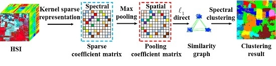
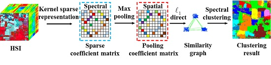
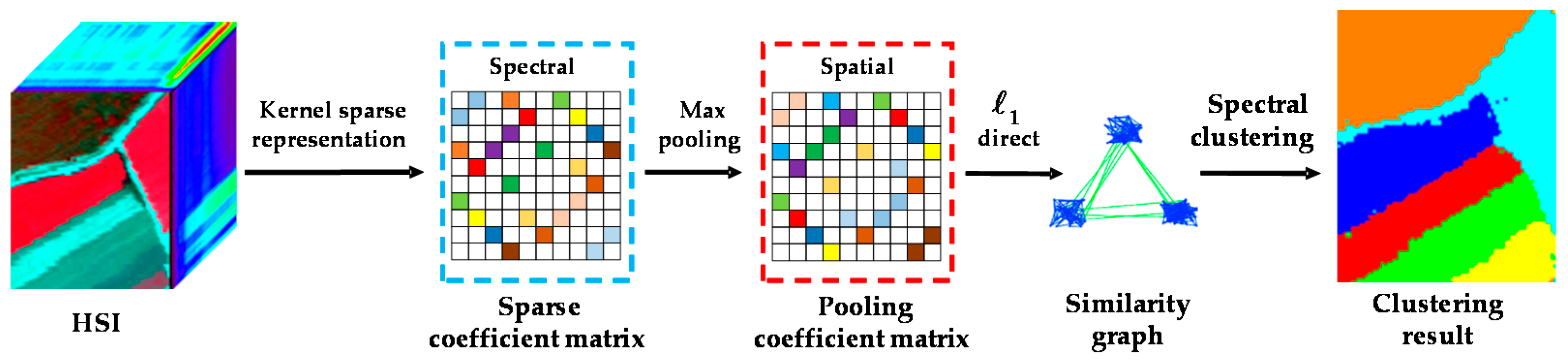
In this paper, to address these issues, we introduce a novel kernel sparse subspace clustering algorithm with a spatial max pooling operation (KSSC-SMP) for hyperspectral remote sensing data interpretation, which is an extension of our previous conference work [21]. The proposed method simultaneously explores the nonlinear structure and the inherent spectral-spatial attributes of HSIs. On the one hand, with the kernel strategy, we map the feature points from the original feature space to a much higher dimensional space to ensure that the linearly inseparable points are more separable. On the other hand, in order to fully exploit the discriminative spectral-spatial information of HSIs and the potential of the SSC model, the spatial max pooling operation is introduced to merge the obtained representation coefficients into new features which incorporate the spatial-contextual information, thereby improving the clustering performance and guaranteeing the spatial homogeneity of the final clustering result.

The rest of this paper is organized as follows. Section 2 reviews the classical SSC model. Section 3 introduces the proposed KSSC-SMP algorithm in detail. Section 4 describes the experimental results. Section 5 analyzes the experimental results. Section 6 draws the conclusions and points out the future research lines.

2. Sparse Subspace Clustering (SSC)

In this section, we briefly review the SSC algorithm. By using the HSI dataset itself as the representation dictionary, the attributes of each data point can be comprehensively exploited within the SSC framework [13]. For an HSI with a size of $M\times N\times p$, all the pixels can be considered as being selected from a union of $l$ affine subspaces $S_1\cup S_2\cup \cdots S_l$ of dimensions ${\left\{d_i\right\}}_{i=1}^l$ in the full space ${ℝ}^p$ with $d_1+d_2+\cdots +d_l=p$, where $M$ denotes the height of the image, $N$ represents the width of the image, and $p$ stands for the number of spectral channels. By treating each pixel as a column vector, the HSI cube can be transformed into a 2-D matrix $Y=\left[y_1,y_2,\cdots ,y_{MN}\right]\in {ℝ}^{p\times MN}$. Then, with this 2-D matrix being utilized as the representation dictionary, the sparse optimization problem can be modeled as follows:

$${\min }_C{\Vert C\Vert }_0 s.t. Y=YC+N,diag\left(C\right)=0,C^{T}1=1$$

(1)

where $C\in {ℝ}^{MN\times MN}$ denotes the representation coefficient matrix, $N\in {ℝ}^{p\times MN}$ stands for the representation error matrix, and $1\in {ℝ}^{MN}$ is a vector whose elements are all ones. The constraint $diag\left(C\right)=0$ is used to eliminate the trivial solution of each pixel being represented as a linear combination of itself [13]. The condition $C^{T}1=1$ means that it adopts the affine subspace model, which is a special linear subspace model [13,15]. As the ${\ell }_0$-norm optimization problem is non-deterministic polynomial hard (NP-hard), the relaxed ${\ell }_1$-norm is usually adopted [22]:

$${\min }_C{\Vert C\Vert }_1 s.t. Y=YC+N,diag\left(C\right)=0,C^{T}1=1$$

(2)

The optimization problem in Equation (2) can be effectively solved by the alternating direction method of multipliers (ADMM) algorithm [23,24,25]. We then construct the similarity graph using the sparse coefficient matrix [15,16,17]. Meanwhile, the symmetric form is adopted to enhance the connectivity of the graph:

$$W=\left|C\right|+{\left|C\right|}^T$$

(3)

where $W\in {ℝ}^{MN\times MN}$ denotes the similarity graph whose element $W_{i,j}$ represents the similarity between pixel $i$ and pixel $j$. The spectral clustering algorithm is then applied to the similarity graph to obtain the final clustering result [26,27,28].

3. Kernel Sparse Subspace Clustering Algorithm with a Spatial Max Pooling Operation (KSSC-SMP)

In this section, we introduce the newly developed KSSC-SMP algorithm. The proposed approach attempts to fully exploit both the nonlinear structure of HSIs and the potential of the SSC model to achieve more accurate clustering results. Considering the complex nonlinear structure of HSIs, we map the feature points to a much higher dimensional kernel space with the kernel strategy to make them linearly separable. In this way, a more accurate representation coefficient matrix can be obtained. In addition, the spatial max pooling operation is introduced to yield new features with these coefficients by incorporating the spatial-contextual information.

3.1. Kernel Sparse Subspace Clustering Algorithm (KSSC)

The kernel sparse subspace clustering (KSSC) algorithm extends the SSC algorithm to nonlinear manifolds by the use of a kernel strategy to map the feature points from the original space to a much higher dimensional space, in order to make them linearly separable [29]. The kernel mapping directly takes the signal in the kernel space as a feature [30] and represents each signal with the others from its own subspace, as in SSC. The sparse representation coefficient matrix can then be obtained by solving the following optimization problem:

$${\min }_C{\Vert C\Vert }_1+\lambda {\Vert {{\rm K}}\left(Y\right)-{{\rm K}}\left(Y\right)C\Vert }_F^2 s.t. diag\left(C\right)=0,C^{T}1=1$$

(4)

where $\lambda$ represents a tradeoff between the data fidelity term and the sparsity term, and ${{\rm K}}:{ℝ}^p\to {{\rm H}}$ is a mapping function from the input space to the reproducing kernel space ${{\rm H}}$ [30]. We let ${{{\rm K}}}_{YY}\in {ℝ}^{MN\times MN}$ denote a positive semi-definite kernel Gram matrix whose elements are computed as follows:

$${\left[{{{\rm K}}}_{YY}\right]}_{i,j}={\left[{\langle {{\rm K}}\left(Y\right),{{\rm K}}\left(Y\right)\rangle }_{{{\rm H}}}\right]}_{i,j}={{\rm K}}{\left(y_i\right)}^T{{\rm K}}\left(y_j\right)=\kappa \left(y_i,y_j\right)$$

(5)

where $y_i$ is the “spectral pixel” at location $i$ in HSI $Y$ and $\kappa :{ℝ}^p\times {ℝ}^p\to ℝ$ represents the kernel function, which measures the similarity of two arguments denoted as a pair of pixels. Commonly used kernels include the radial basis function (RBF) kernel $\kappa \left(y_i,y_j\right)=\exp \left(-\delta {\Vert y_i-y_j\Vert }^2\right)$ and the polynomial kernel $\kappa \left(y_i,y_j\right)={\langle \langle y_i,y_j\rangle +a\rangle }^b$, where $\delta$, $a$, and $b$ are the parameters of the kernel functions. In this paper, the RBF kernel is adopted. As the feature space of the RBF kernel has an infinite number of dimensions, and its value decreases with distance between (0, 1), it can be readily interpreted as a similarity measure [30].

3.2. Incorporating Spatial Information with the Spatial Max Pooling Operation

Through sparse representation, the coefficients can reveal the underlying cluster structure and can be directly utilized as features. However, when only using spectral information, a single representation coefficient vector of the target pixel can only provide limited discriminative information [31,32]. Based on the fact that pixels within a local patch (where the center pixel is the target pixel to be processed) have a high probability of being associated with the same thematic class, the sparse representation coefficients of these pixels are also expected to be similar. Therefore, the spatial pooling operation can be considered a reasonable way to merge these similar sparse representation coefficient vectors and yield a new feature vector with better discriminative ability, which is an approach that has been widely used in the literature [33,34].

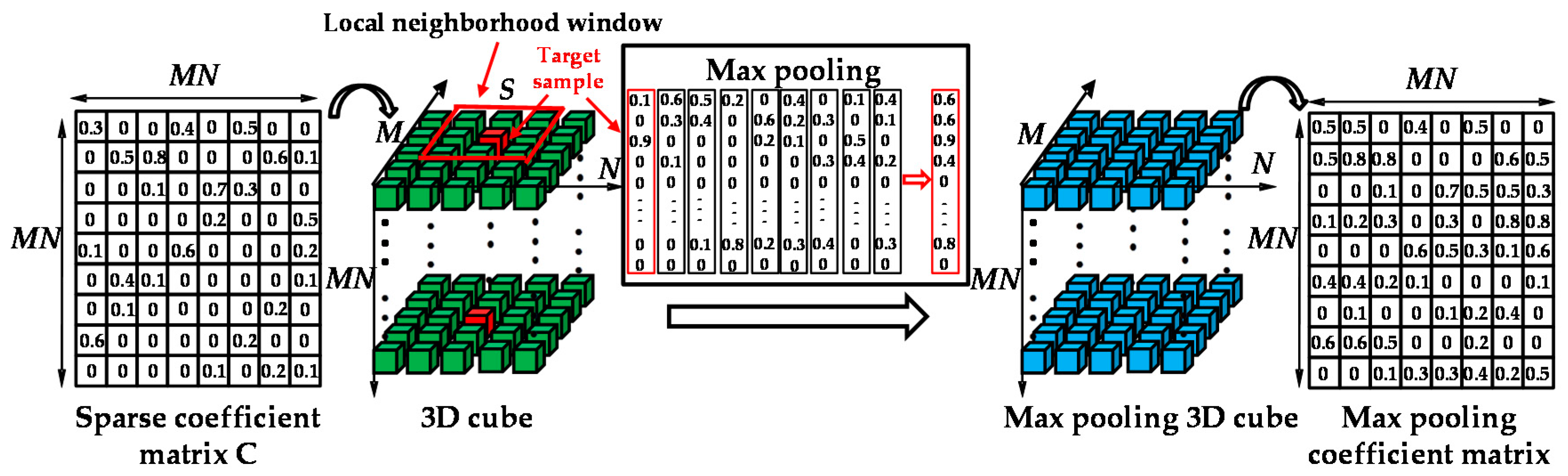
At this point, considering the mechanism adopted by SSC (which pays more attention to larger coefficients and tends to highlight their role), the spatial max pooling operation is adopted to merge these sparse coefficient vectors into a new pooling vector, which suppresses the small elements and preserves the large ones. This is because the larger the representation coefficients, the more similar to the target pixel the corresponding representation atoms are, and the greater the contribution they make to the sparse representation of the target pixel. In this process, since all the representation coefficients within the local patch are simultaneously taken into consideration to generate a new representation coefficient vector, the spatial-contextual information can be naturally incorporated. Moreover, it should be noted that the spatial max pooling operation is performed in the representation dimension, not directly on the pixel values.

Firstly, the 2-D sparse coefficient matrix $C\in {ℝ}^{MN\times MN}$ is reshaped into a 3-D cube $\widehat{C}\in {ℝ}^{M\times N\times MN}$ along rows, which can be seen as a “coefficient hyperspectral cube”. We then consider a local neighborhood window of size $S$ for each representation coefficient vector, with the currently processed one as the center. Following this, the max pooling operation is performed on the local neighborhood window to select the local largest coefficient value of each band to act as one element of the newly generated coefficient vector for the target pixel. In this way, the more meaningful and discriminative information among the local neighborhood is extracted by the newly generated sparse representation coefficient vector, and the spatial-contextual information is naturally incorporated and fused in the max pooling process to generate the new spectral-spatial features. Finally, the obtained coefficient features are utilized to cluster the HSI. The process of spatial max pooling is illustrated in Figure 1.

3.3. The KSSC-SMP Algorithm

In order to further improve the clustering performance, we combine the two aforementioned schemes into a unified framework to obtain the KSSC-SMP algorithm, which can simultaneously deal with the complex nonlinear structure and utilize the spectral-spatial attributes of HSIs. The KSSC-SMP algorithm can be summarized as shown in Algorithm 1.

Algorithm 1. The kernel sparse subspace clustering algorithm with a spatial max pooling operation (KSSC-SMP) for hyperspectral remote sensing imagery

Input: 1) A 2-D matrix of the HSI containing a set of points ${\left\{y_i\right\}}_{i=1}^{MN}$, in a union of $l$ affine subspaces ${\left\{S_i\right\}}_{i=1}^l$; 2) Parameters, including the cluster number $l$, the regulation parameter $\lambda$, the kernel parameter $\delta$, and the window size $S$ of the spatial max pooling operation. Main algorithm: 1) Construct the kernel sparse representation optimization model (Equation (4)) and solve it to obtain the kernel sparse representation coefficient matrix $C$ using ADMM; 2) Conduct the spatial max pooling operation on $C$ to obtain the max pooling coefficient matrix , as shown in Figure 1; 3) Construct the similarity graph with the max pooling coefficient matrix; 4) Apply spectral clustering to the similarity graph to obtain the final clustering results; Output: A 2-D matrix which records the labels of the clustering result of the HSI.

The flowchart of the proposed KSSC-SMP algorithm is given in Figure 2.

4. Experimental Results

In order to evaluate the effectiveness of the proposed KSSC-SMP algorithm, the following state-of-the-art clustering approaches were implemented for comparative purposes: FCM-S1 [8], clustering by fast search and find of density peaks (CFSFDP) [35], SSC [13], S⁴C [15], and L2-SSC [16]. The number of clusters was determined by carefully observing the original image, and the parameters of each clustering method were carefully optimized through the well-known grid search strategy. The thematic information was manually determined to give a label for each cluster group through cross-referencing between the clustering result and the original image. To thoroughly evaluate the performance of each clustering method, both the visual cluster map and quantitative evaluation measures are provided, including the accuracy for each class (producer’s accuracy), the overall accuracy (OA), the kappa coefficient, the z-value, and the running time.

The confusion matrix is defined as shown in

Table 1. Confusion matrix of an algorithm.

	Predicted Class	1	$\cdots$	i	$\cdots$	j	$\cdots$	l	Row Total
Actual Class
1		$p_{1,1}$	$\cdots$	$p_{1,i}$	$\cdots$	$p_{1,j}$	$\cdots$	$p_{1,l}$	$p_{1,+}$
$⋮$		$⋮$	$⋮$	$⋮$	$⋮$	$⋮$	$⋮$	$⋮$	$⋮$
i		$p_{i,1}$	$\cdots$	$p_{i,i}$	$\cdots$	$p_{i,j}$	$\cdots$	$p_{i,l}$	$p_{i,+}$
$⋮$		$⋮$	$⋮$	$⋮$	$⋮$	$⋮$	$⋮$	$⋮$	$⋮$
j		$p_{j,1}$	$\cdots$	$p_{j,i}$	$\cdots$	$p_{j,j}$	$\cdots$	$p_{j,l}$	$p_{j,+}$
$⋮$		$⋮$	$⋮$	$⋮$	$⋮$	$⋮$	$⋮$	$⋮$	$⋮$
l		$p_{l,1}$	$\cdots$	$p_{l,i}$	$\cdots$	$p_{l,j}$	$\cdots$	$p_{l,l}$	$p_{l,+}$
Column total		$p_{+,1}$	$\cdots$	$p_{+,i}$	$\cdots$	$p_{+,j}$	$\cdots$	$p_{+,l}$	MN

l: the number of classes; MN: the total number of pixels; i: the ith class; $p_{i,j}$: the number of pixels that are actually class i but predicted as class j, where $1\le i,j\le l$; $p_{i,+}$: the number of the pixels predicted as class i; $p_{+,i}$: the number of pixels of actual class i.

, which is a specific table layout that allows visualization of the performance of an algorithm. In the clustering field, it is commonly called a “matching matrix”. Based on the confusion matrix, the producer’s accuracy, OA, and kappa are calculated as follows.

$$Producer\text{'}saccuracy:p_i=\frac{p_{i,i}}{p_{i,+}}$$

(6)

$$\mathrm{OA}=\frac{{\displaystyle \sum _{i=1}^l{p}_{i,i}}}{MN}$$

(7)

$$Kappa=\frac{MN{\displaystyle \sum _{i=1}^l{p}_{i,i}-{\displaystyle \sum _{i=1}^l\left(p_{i,+}\cdot p_{+,i}\right)}}}{{\left(MN\right)}^2-{\displaystyle \sum _{i=1}^l\left(p_{i,+}\cdot p_{+,i}\right)}}$$

(8)

where $p_i$ refers to the producer’s accuracy of the ith class. The z-value measure is based on the contingency table, as shown in

Table 2. Contingency table of two different clustering methods.

Algorithm Test	Algorithm 2 Positive	Algorithm 2 Negative	Row Total
Algorithm 1 positive	$f_{1,1}$	$f_{1,2}$	$f_{1,1}+f_{1,2}$
Algorithm 1 negative	$f_{2,1}$	$f_{2,2}$	$f_{2,1}+f_{2,2}$
Column total	$f_{1,1}+f_{2,1}$	$f_{1,2}+f_{2,2}$	$f_{1,1}+f_{1,2}+f_{2,1}+f_{2,2}$

$f_{1,1}$: the number of pixels that both algorithms classified correctly; $f_{1,2}$: the number of pixels that Algorithm 1 classified correctly but Algorithm 2 misclassified; $f_{2,1}$: the number of pixels that Algorithm 2 classified correctly but Algorithm 1 misclassified; $f_{2,2}$: the number of pixels that both algorithms misclassified.

, and it can be calculated as follows [36].

$$z=\frac{f_{1,2}-f_{2,1}}{\sqrt{f_{1,2}+f_{2,1}}}$$

(9)

where $z$ represents the significance of the difference between the two clustering algorithms.

4.1. Experimental Results Obtained with the Salinas Image

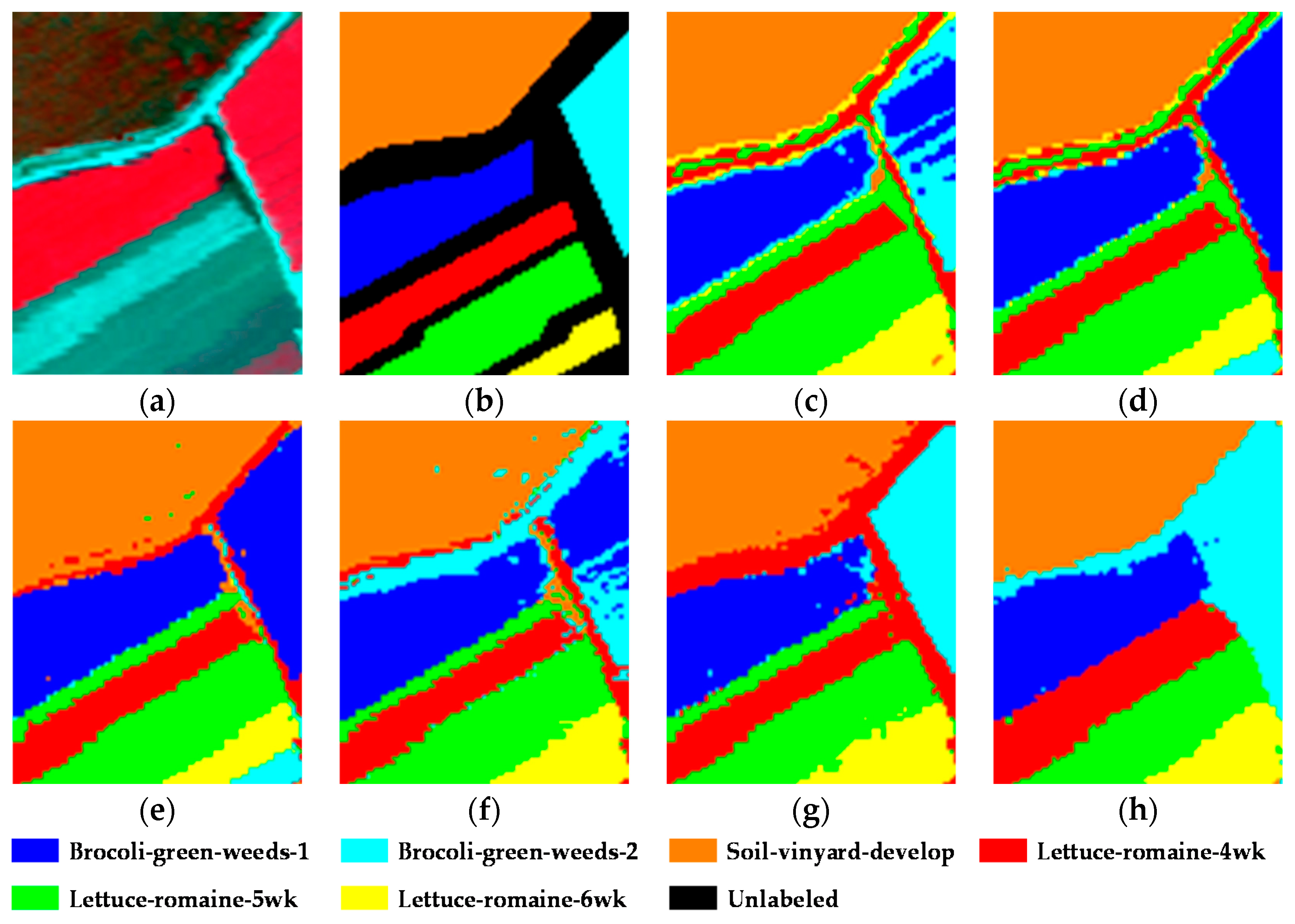
The first experiment was conducted on the well-known Salinas image. This scene was acquired by the Airborne Visible/Infrared Imaging Spectrometer (AVIRIS) sensor over the Salinas Valley, CA, USA, and consists of 512 × 217 pixels and 224 spectral reflectance bands in the wavelength range of 0.4–2.5 um. Twenty bands (108–112, 154–167, and 224) corresponding to water absorption and noisy bands were removed, leaving 204 bands for the experiment. In this scene, there are 16 different classes, which are mainly different kinds of vegetation. A typical area at a size of 100 × 80 was selected as the test data, containing six main land-cover classes: Brocoli-green-weeds-1 (Brocoli-1), Brocoli-green-weeds-2 (Brocoli-2), Soil-vinyard-develop (Soil), Lettuce-romaine-4wk (Lettuce-4wk), Lettuce-romaine-5wk (Lettuce-5wk), and Lettuce-romaine-6wk (Lettuce-6wk). To be consistent with all the unsupervised methods, all the samples in the ground truth were utilized as the test samples. The false-color composite image and the ground truth are shown in Figure 3a,b, respectively. The parameters of each clustering algorithm in this experiment were set as shown in

Table 3. Parameters of each clustering method for the Salinas image: fuzzy c-means with spatial information (FCM-S1), clustering by fast search and find of density peaks (CFSFDP), sparse subspace clustering (SSC), spectral-spatial sparse subspace clustering (S⁴C), ${\ell }_2$-norm regularized sparse subspace clustering (L2-SSC), and kernel sparse subspace clustering with a spatial max pooling operation (KSSC-SMP).

Method	Salinas
FCM-S1	$l=6$, $e=2$, $\alpha =0.9$
CFSFDP	---
SSC	$l=6$, $\lambda =2.63\times {10}^{-6}$
S4C	$l=6$, $\lambda =8.78\times {10}^{-7}$, $\alpha =5\times {10}^3$, $S=3$
L2-SSC	$l=6$, $\lambda =3.07\times {10}^{-6}$, $\alpha =3\times {10}^3$
KSSC-SMP	$l=6$, $\lambda =3.07\times {10}^{-6}$, $\delta ={10}^{-7}$, $S=3$

$l$: cluster number; $e$: fuzzy exponential; $\lambda$: tradeoff parameter; $\alpha$: tradeoff parameter; $\delta$: kernel parameter; $S$: window size parameter.

.

The thematic maps obtained by each clustering algorithm with the Salinas image and the corresponding quantitative evaluation of the clustering precision are provided in Figure 3 and

Table 4. Quantitative evaluation of the different clustering algorithms for the Salinas image: the best result in each row is shown in bold, with the second-best result underlined.

Method	Class	FCM-S1	CFSFDP	SSC	S4C	L2-SSC	KSSC-SMP
Producer’s accuracy (%)	Brocoli-1	99.01	100	99.90	99.51	98.72	100
	Brocoli-2	46.93	0	0	31.75	100	100
	Soil	97.10	97.96	99.49	97.30	95.32	99.95
	Lettuce-4wk	93.39	93.95	94.23	93.67	95.08	100
	Lettuce-5wk	100	100	100	100	94.84	99.46
	Lettuce-6wk	100	95.20	93.45	100	100	100
Overall accuracy (OA) (%)		91.64	86.44	86.93	90.04	96.58	99.89
Kappa		0.8922	0.8241	0.8301	0.8731	0.9563	0.9986
z-value		13.2343	−4.4388	0	10.3494	18.6001	26.5168
Time (s)		59.11	75.52	9.24 × 102	9.59 × 102	8.95 × 102	3.81 × 102

, respectively. In Table 4, the best result in each row is shown in bold, with the second-best result underlined. From the figure and the table, it can be clearly observed that the proposed KSSC-SMP algorithm significantly improves the clustering performance and is superior to the other state-of-the-art clustering methods. KSSC-SMP achieves an optimal or sub-optimal precision for all the classes. As a result, it achieves the best OA of 99.89% and kappa of 0.9986.

4.2. Experimental Results Obtained with the University of Pavia Image

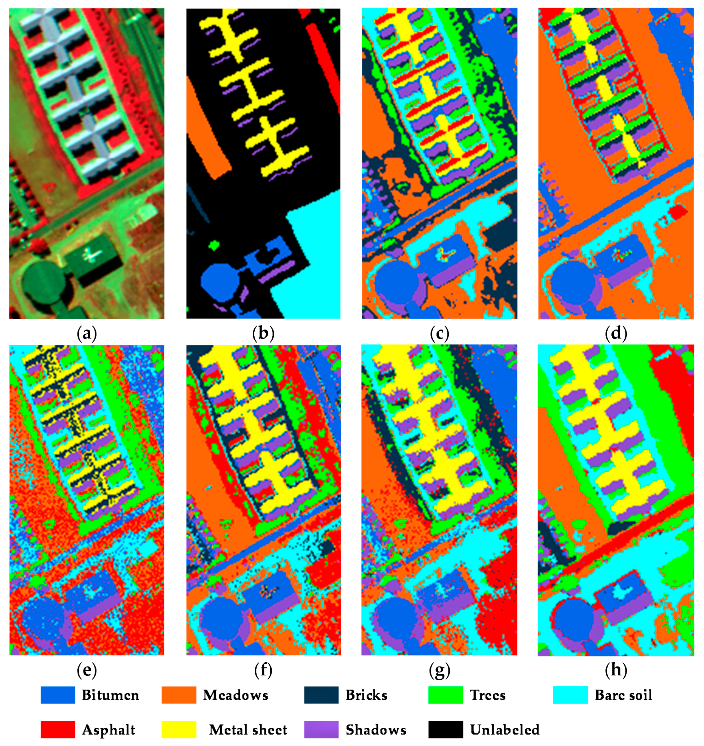
The second experimental dataset was the University of Pavia image scene, which was collected by the Reflective Optics System Imaging Spectrometer (ROSIS) sensor during a flight campaign over Pavia, Northern Italy. This image has 610 × 340 pixels, with 103 spectral reflectance bands utilized in the experiment after removing the water absorption and noisy bands. The geometric resolution of this image is 1.3 m, with nine classes contained in the scene. Considering the computational complexity, a typical sub-set at a size of 200 × 100 was utilized as the test data [15,16,17], with eight main land-cover classes: Metal sheet, Asphalt, Meadows, Trees, Bare soil, Bitumen, Bricks, and Shadows. All the samples in the ground truth were utilized as the test samples. The composite false-color image and the corresponding ground truth are provided in Figure 4a,b. Differing from the first experimental dataset, this scene is of a typical city area that has a more complex distribution of land-cover classes. The parameters of each clustering algorithm in this experiment were set as shown in

Table 5. Parameters of each clustering method for the University of Pavia image: fuzzy c-means with spatial information (FCM-S1), clustering by fast search and find of density peaks (CFSFDP), sparse subspace clustering (SSC), spectral-spatial sparse subspace clustering (S⁴C), ${\ell }_2$-norm regularized sparse subspace clustering (L2-SSC), and kernel sparse subspace clustering with a spatial max pooling operation (KSSC-SMP).

Method	University of Pavia
FCM-S1	$l=8$, $e=2$, $\alpha =0.9$
CFSFDP	---
SSC	$l=8$, $\lambda =1.58\times {10}^{-5}$
S4C	$l=8$, $\lambda =1.58\times {10}^{-5}$, $\alpha =3.0\times {10}^3$, $S=3$
L2-SSC	$l=8$, $\lambda =1.58\times {10}^{-5}$, $\alpha =9\times {10}^3$
KSSC-SMP	$l=8$, $\lambda =1.58\times {10}^{-5}$, $\delta ={10}^{-8}$, $S=3$

$l$: cluster number; $e$: fuzzy exponential; $\lambda$: tradeoff parameter; $\alpha$: tradeoff parameter; $\delta$: kernel parameter; $S$: window size parameter.

.

The cluster maps of the University of Pavia image obtained by each algorithm are shown in Figure 4, with the corresponding quantitative evaluation provided in

Table 6. Quantitative evaluation of the different clustering algorithms for the University of Pavia image. The best result in each row is shown in bold, with the second-best result underlined.

Method	Class	FCM-S1	CFSFDP	SSC	S4C	L2-SSC	KSSC-SMP
Producer’s accuracy (%)	Metal sheet	60.99	37.26	53.84	99.09	97.34	99.85
	Asphalt	0	0	0.71	0	0.71	100
	Meadows	87.37	100	52.60	99.09	92.97	99.09
	Trees	58.73	0	100	87.30	60.32	100
	Bare soil	24.97	21.41	22.04	31.93	37.20	51.58
	Bitumen	100	100	85.58	98.37	87.67	95.47
	Bricks	0	0	0	60.64	0	98.94
	Shadows	99.72	100	98.61	98.61	93.91	100
Overall accuracy (OA) (%)		52.27	46.97	43.97	65.09	63.30	80.02
Kappa		0.4484	0.3874	0.3495	0.5852	0.5618	0.7583
z-value		21.9698	6.8536	0	36.5971	34.1658	48.1975
Time (s)		3.69 × 102	4.81× 102	1.29 × 104	7.40 × 103	1.33 × 104	1.98 × 103

. For consistency, the best result in each row is shown in bold and the second-best result is underlined. In this experiment, it can be clearly seen that the clustering results are consistent with those of the first experiment, and similar conclusions can be drawn. In this experiment, the proposed KSSC-SMP, again, achieves the best clustering performance in both the visual and quantitative evaluations.

5. Discussion

5.1. Experimental Results Analysis

From Figure 3 and Figure 4 and Table 4 and Table 6, it can be clearly observed that the clustering performance of FCM-S1 is far from satisfactory, as this clustering model assumes that each cluster satisfies a convex “ball-like” distribution, and it cannot handle the large spectral variability of HSIs [15]. As a result, misclassification and within-class noise appear in the cluster maps. Compared with FCM-S1, CFSFDP performs even more poorly with a higher level of misclassification, with only a few classes effectively recognized. This suggests that the density-based segmentation strategy does not fit well with the complex structure of HSIs. Specifically, both these methods completely fail to recognize the Asphalt and Bricks classes in the second experiment.

We now compare the clustering results of the SSC algorithm and its extensions. Due to the fact that it ignores the spatial information, the clustering results of SSC are far from satisfactory, with a large amount of salt-and-pepper noise and numbers of misclassifications. Although SSC successfully distinguishes most of the classes in the first experiment, showing great potential for hyperspectral clustering, it performs very badly in the second experiment and obtains the lowest clustering precision. Compared with SSC, S⁴C effectively improves the clustering performance, by utilizing the spectral weighting strategy to guarantee that highly correlated pixels occupy the dominant place in the representation process, and incorporates the spatial neighborhood information with the local averaging constraint. For example, in the first experiment, the recognition precision of Brocoli-green-weeds-2 and Lettuce-romaine-6wk is improved from 0% and 93.45% to 31.75% and 100%, respectively. On the other hand, L2-SSC also obtains a much better clustering precision than that of the original SSC method, which again suggests the importance of the spatial information from another perspective. However, due to the limitations of the linear representation, there are still some classes that are not effectively recognized by these two methods, such as the Asphalt and Bricks classes in the second experiment. Compared with the three linear methods, the proposed KSSC-SMP algorithm further improves the clustering performance by exploiting the nonlinear structure of the HSI and generating more discriminative features by incorporating the spatial-contextual information with the spatial max pooling operation. For example, in the second experiment, for the Asphalt and Bricks classes, which are beyond the recognition capability of most of the methods, the recognition precision of KSSC-SMP is 100% and 98.94%, respectively, which suggests the superiority of the nonlinear method. As a result, KSSC-SMP achieves much smoother cluster maps with a much higher clustering precision in both experiments, which confirms the superiority of the nonlinear method. Increments in OA of approximately 13%, 9%, and 3% are achieved in the first experiment, compared with that of SSC, S⁴C, and L2-SSC, respectively, and increments in OA of approximately 26%, 15%, and 17% are achieved in the second experiment. Overall, KSSC-SMP outperforms the other state-of-the-art clustering methods and achieves the best clustering performance in both the visual and quantitative evaluations.

In order to reflect the significant difference between the clustering methods, we took the clustering result of SSC as the baseline and calculated the z-values [36] of the other clustering results. For the widely used 5% level of significance, we consider that there is a significant difference between the two clustering methods if |z| >3.84. From Table 4 and Table 6, it can be clearly observed that S⁴C and L2-SSC perform significantly better than the original SSC algorithm. In addition, the proposed KSSC-SMP algorithm also performs significantly better than the linear methods. On the other hand, from the last rows of Table 4 and Table 6, it can be seen that the four SSC-based algorithms require more computation time than CFSFDP and FCM-S1, but they do provide better clustering accuracies. Fortunately, with the development of computer hardware and the parallel computing technique, this will not be a major problem for much longer.

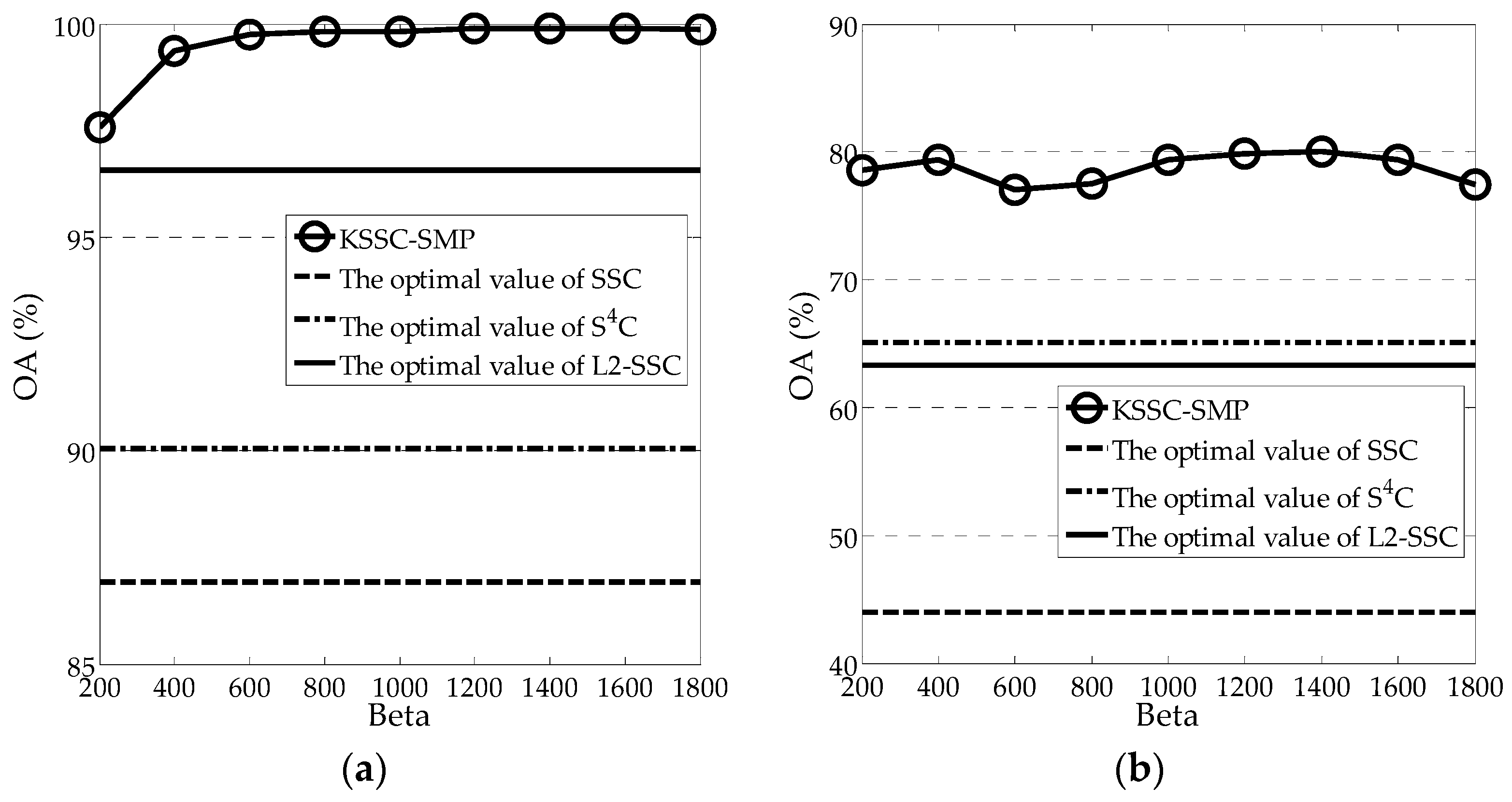
5.2. Sensitivity Analysis of the Parameters

There are three parameters in the proposed KSSC-SMP algorithm: the regularization parameter $\lambda$, the kernel parameter $\delta$, and the window size parameter $S$. When analyzing one parameter, the other two parameters were fixed at the optimal values. Both the AVIRIS Salinas image scene and the University of Pavia image scene were utilized to test the sensitivity of the parameters of KSSC-SMP.

As a tradeoff between the data fidelity term and the sparsity term, the sensitivity of the regularization parameter $\lambda$ was first analyzed. For this parameter, we adopted the same strategy that was used with the other SSC-based methods in [13,15]. In practice, parameter $\lambda$ is decided by the following formulation [15]:

$$\lambda =\frac{\beta }{\mu }$$

(10)

$$\mu \triangleq \underset{i}{\min } \underset{j\ne i}{\max }\left|y_i^T{y}_j\right|$$

(11)

where $\beta$ is a coefficient, and $\mu$ can be exactly computed for each dataset.

From Equations (10) and (11), it can be easily found that the sensitivity of $\lambda$ is actually decided by $\beta$, as $\mu$ is fixed for a certain dataset. Therefore, in practice, we only need to fine tune $\beta$. Figure 5 shows the compromise between OA and $\beta$ for both experimental images. In Figure 5, the optimal clustering values of SSC, S⁴C, and L2-SSC are also provided. From the figure, it can be observed that $\beta$ is independent of the dataset, to some degree, as the optimal value always falls into a relatively narrow range of [1000, 1400]. For a certain dataset, $\beta$ can be easily fine-tuned. In addition, it should be noted that KSSC-SMP always achieves a much better precision than the optimal values of the other three linear SSC-based methods, which further demonstrates its effectiveness.

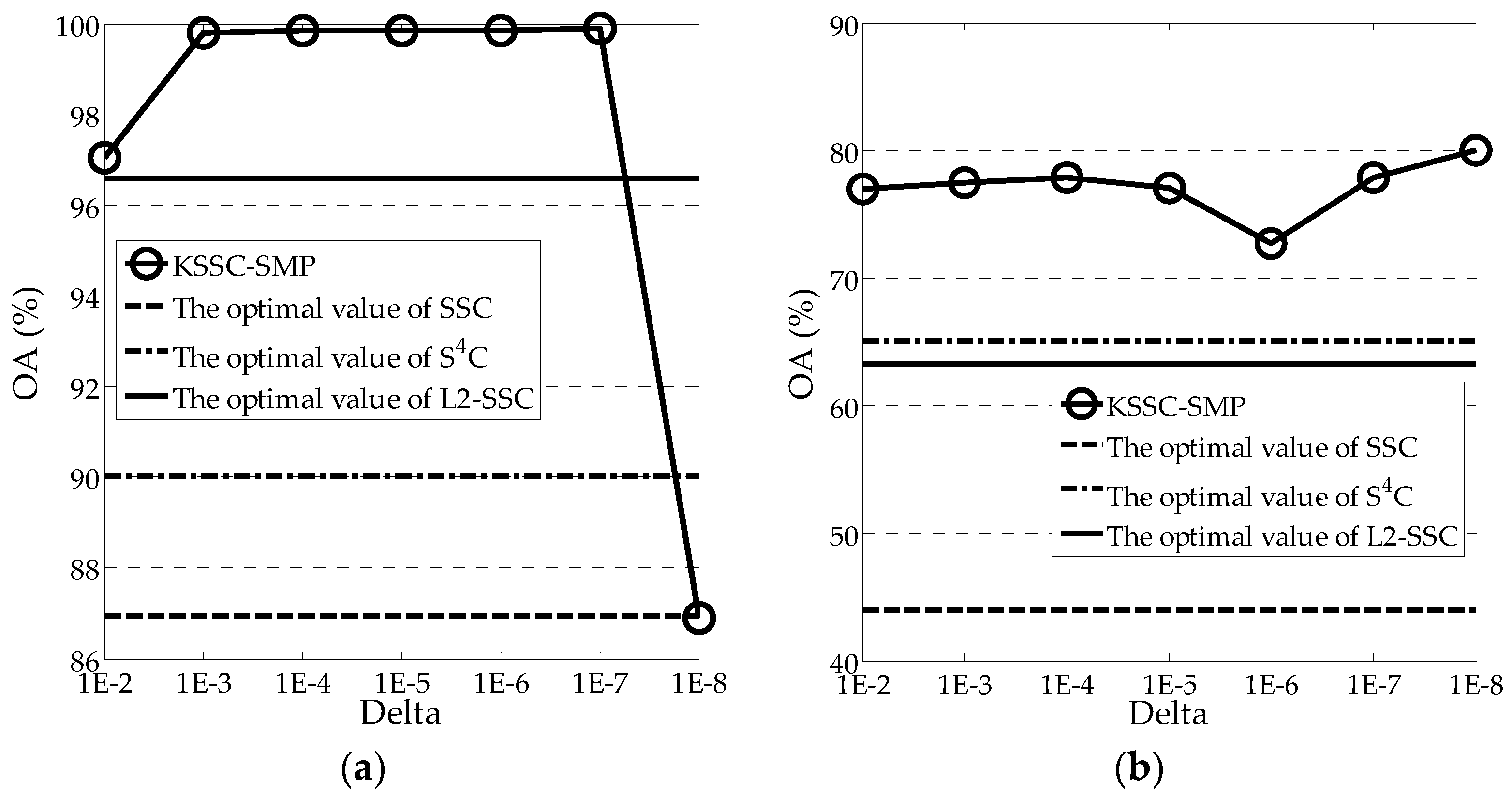
The kernel parameter $\delta$ controls the quality of the projection of the feature points from the original space to the kernel space, and is quite important for the proposed KSSC-SMP algorithm. Similarly, the sensitivity of the kernel parameter was analyzed through a series of experiments, as shown in Figure 6. From the figure, it can be seen that the KSSC-SMP algorithm is relatively robust for this parameter, and its performance is relatively stable. The optimal value of $\delta$ varies for the different datasets. For the Salinas image, the optimal value is 1 × 10⁻⁷, and for the University of Pavia image, it is 1 × 10⁻⁸. However, it can be seen that over a very large range of $\delta$, KSSC-SMP can achieve a better performance than the three linear methods. Therefore, the KSSC-SMP algorithm is suitable for use in real applications.

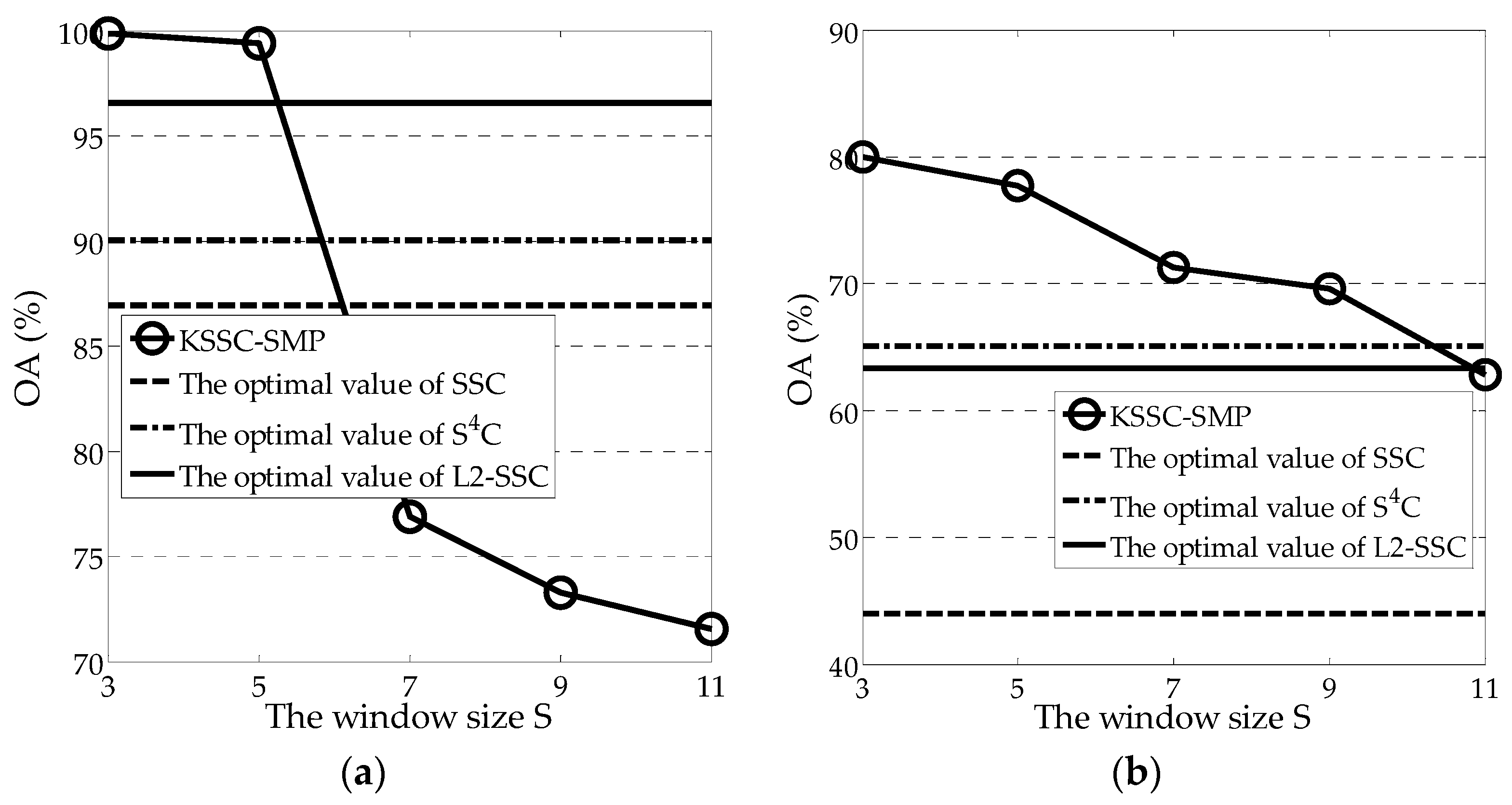
The window size parameter $S$ controls the spatial max pooling operation. The influence of this parameter on the clustering performance is shown in Figure 7, using a similar strategy to that adopted for the other two parameters. From the figure, it can be seen that the spatial information plays a very important role in the clustering process. For both experimental scenes, the optimal value of parameter $S$ is 3. Both these scenes have a relatively complex distribution of land-cover classes. Generally, parameter $S$ is closely related to the resolution of the image. Again, over a large range of parameter $S$, KSSC-SMP can achieve a better clustering performance than the three linear methods, which further confirms its effectiveness.

6. Conclusions and Future Lines of Research

In this paper, we have proposed a new kernel sparse subspace clustering algorithm with a spatial max pooling operation (KSSC-SMP) for HSI data interpretation. The proposed approach focuses on exploiting the complex nonlinear structure of HSIs and obtaining a more precise representation coefficient matrix with the kernel sparse representation. In addition, the spatial max pooling operation is introduced to these coefficients to yield new features to fully exploit the discriminative spectral-spatial information of HSIs and the potential of the SSC model. Thereby, KSSC-SMP can effectively improve the clustering performance and guarantee the spatial homogeneity of the final clustering result.

Although the results show that the KSSC-SMP algorithm is very competitive, there are several aspects that could be improved. For instance, the method could be further improved by adaptively determining the regularization parameters and allowing for the extraction of more discriminative spatial features. All of these issues will be addressed in our future work.