Object-Based Detection of Lakes Prone to Seasonal Ice Cover on the Tibetan Plateau

Abstract

The Tibetan Plateau, the world’s largest orogenic plateau, hosts thousands of lakes that play prominent roles as water resources, environmental archives, and sources of natural hazards such as glacier lake outburst floods. Previous studies have reported that the size of lakes on the Tibetan Plateau has changed rapidly in recent years, possibly because of atmospheric warming. Tracking these changes systematically with remote sensing data is challenging given the different spectral signatures of water, the potential for confusing lakes with glaciers, and difficulties in classifying frozen or partly frozen lakes. Object-based image analysis (OBIA) offers new opportunities for automated classification in this context, and we have explored this method for mapping lakes from LANDSAT images and Shuttle Radar Topography Mission (SRTM) elevation data. We tested our algorithm for most of the Tibetan Plateau, where lakes in tectonic depressions or blocked by glaciers and sediments have different surface colours and seasonal ice cover in images obtained in 1995 and 2015. We combined a modified normalised difference water index (MNDWI) with OBIA and local topographic slope data in order to classify lakes with an area >10 km². Our method derived 323 water bodies, with a total area of 31,258 km², or 2.6% of the study area (in 2015). The same number of lakes had covered only 24,892 km² in 1995; lake area has increased by ~26% in the past two decades. The classification had estimated producer’s and user’s accuracies of 0.98, with a Cohen’s kappa and F-score of 0.98, and may thus be a useful approximation for quantifying regional hydrological budgets. We have shown that our method is flexible and transferable to detecting lakes in diverse physical settings on several continents with similar success rates.

1. Introduction

The Tibetan Plateau is the world’s largest orogenic plateau, with a mean elevation of more than 4000 m above sea level (a.s.l.), and is known as “the Roof of the World” or “the 3rd Pole of the Earth” [1,2,3]. The Plateau is surrounded by the Himalayas to the south, the Kunlun Shan to the north, the Pamir to the west, and the Qilian Shan to the northeast [4]. Together with these ranges, the Tibetan Plateau serves as “the Water Tower of Asia” [5,6,7], hosting glaciers and thousands of lakes that play prominent roles as water resources, environmental archives, and potential sources of natural hazards, such as glacier lake outburst floods [8].

The Tibetan Plateau is among the most sensitive places to atmospheric warming [9]. Temperatures on the plateau have risen by 0.3 °C per decade—three times the global average [1,10]. Symptoms attributed to atmospheric warming on the plateau include retreating glaciers [4,11], degrading permafrost [1,12], and rapidly changing lake areas [13]. The glaciers in the surrounding mountain ranges are prone to changing hydrological and meteorological conditions, potentially contributing to changes in the size of the Plateau’s lakes [7]. Many studies have tried to detect and monitor these changes [9,14,15,16,17]. Some researchers [2,11] have argued that the meltwater from glaciers largely drives the size distribution of these lakes. Ground surveys [18] help to verify the changes in detail; however, such field measurements are difficult, expensive, and time-consuming for large regions, especially if needed regularly. Here, satellite-based monitoring offers a solution in terms of repeated and standardised images of lakes, their surface colour, and seasonal ice cover.

Yang and Lu [13] used LANDSAT images covering several decades to capture how the size of lakes on the Tibetan Plateau has changed. Seasonal changes in size are evident for at least 105 lakes [19], with those in the south, central, and northeastern parts of the plateau having higher water levels between March and October, but showing almost no changes between November and February. Many lakes in the north, however, have lower water levels in the warm season, mainly because of strong evaporation and low precipitation. Ma et al. [20] reported that between 1960 and 2006, most existing lakes grew in size, while 60 new lakes >1 km² appeared on the Tibetan Plateau and surrounding areas. Fang et al. [21] revealed different trends in how 35 lakes changed over the past 40 years. For example, Siling Co, the largest lake on the plateau, has increased by >600 km², whereas lakes in the Himalayas have shrunk; lakes in the north and northeastern Tibetan Plateau mainly grew. A local study of Nam Co reported that this lake expanded by 51.8 km² between 1970 and 2010 [22], owing to increasing annual precipitation, air temperature, and runoff, and decreasing evaporation, similar to trends of other lakes such as Siling Co, Bam Co, Pung Co, Darab Co, and Zige Tangco [23].

Few methods of detecting lakes and their changes on the Tibetan Plateau have been developed further. Li et al. [24] proposed an algorithm applying a normalised difference water index, topographic slope, and hillshading to discern glacial lakes from shadows on LANDSAT ETM+ images. They found that pixels classified as water were bimodally distributed, as opposed to pixels representing other land cover, and thus distinct from melting glaciers and shadows. Song et al. [6] estimated changes in lake-water storage on the Tibetan Plateau from the early 1970s to 2011. Using LANDSAT images and ICESat altimetry data, they reported an increase in lake areas and total water storage. They noted a more positive water balance in the northern and central plateau, but a decreasing water balance in the southeastern part, mostly related to glacier melt. Comparable results [17,25] from ICESat data apply to level changes for 154 lakes on the Tibetan Plateau between 2003 and 2009.

Systematically tracking lake changes offers new challenges and opportunities for automatic classification methods, such as object-based image analysis (OBIA) [26]. Such automatic mapping of landforms reduces the operator bias produced by manual digitisation, and allows rapid investigation of large regions. The training of OBIA algorithms requires careful design, however, especially for areas like the Tibetan Plateau, where simple thresholding frequently confuses lakes with glaciers, ice and cloud cover, or highly reflecting sediments. We address this issue and present an OBIA approach to classifying large lakes on the Tibetan Plateau based on LANDSAT images and the Shuttle Radar Topography Mission (SRTM) digital elevation model (DEM). Our objective was to find a suitable workflow using an object-based approach for detecting large lakes based on a water index and digital topography, aiming for a metric insensitive to glaciers and ice cover, running water, or mountain shadows. We present here a method for rapidly delineating lake boundaries and for examining general trends in lakes size for a large area, such as the Tibetan Plateau. Specifically, we used a modified normalised difference water index (MNDWI) [27] to detect water pixels, and OBIA to extract lake boundaries and distinguish them from rivers and glaciers. We then further tested whether our method is readily applicable to classifying lakes of different origins and in different environmental settings elsewhere.

2. Previous Work

Remote sensing data are indispensable for delineating surface objects and tracking how they change [28,29,30]. The continuity of data collection with set parameters [31] enables consistent and accurate long-term analyses. Satellite images have a long tradition in classifying water [32,33,34], streams [35], changes in lake volumes [36], and lake monitoring [37].

2.1. Thresholding Methods

Methods for automatically detecting water bodies from remote sensing data use various spectral properties of water [2,38]. The most common approach uses thresholds on a single band or a ratio of bands, and is easy, quick, and quite accurate in delineating boundaries of water bodies [2,39]. Frazier and Page [32] were among the first to use density slicing on a single band (ρ) of LANDSAT 5 TM images, determining the optimal threshold on each band (i.e., ${\rho }_{Blue}$, ${\rho }_{Green}$, ${\rho }_{Red}$, ${\rho }_{NIR}$ (ρ near-infrared), ${\rho }_{SWIR1}$ (ρ short-wave infrared), and ${\rho }_{SWIR2}$ (ρ short-wave infrared)). They found that ${\rho }_{SWIR1}$ offered the most accurately classified water areas, only marginally inferior to those obtained via a more costly maximum likelihood-based approach to slicing six bands in total. McFeeters [40] introduced a band-ratio method for separating water from other land cover classes. His normalised difference water index (NDWI) [40] makes assumptions similar to those used for computing the normalised difference vegetation index (NDVI) [41] (

Table 1. Band-ratio indices proposed in previous studies to classify vegetation and water.

Index	Equation	Author
Normalised Difference Vegetation Index	NDVI = (${\rho }_{NIR}$ − ${\rho }_{Red}$)/(${\rho }_{NIR}$ + ${\rho }_{Red}$)	Townshend and Justice [41]
Normalised Difference Water Index	NDWI = (${\rho }_{Green}$ − ${\rho }_{NIR}$)/(${\rho }_{Green}$ + ${\rho }_{NIR}$)	McFeeters [40]
Normalised Difference Water Index	NDWI = (${\rho }_{Red}$ − ${\rho }_{SWIR1}$)/(${\rho }_{Red}$ + ${\rho }_{SWIR1}$)	Rogers and Kearny [42]
Modified Normalised Difference Water Index	MNDWI = (${\rho }_{Green}$ − ${\rho }_{SWIR1}$)/(${\rho }_{Green}$ + ${\rho }_{SWIR1}$)	Xu [27]
Automated Water Extraction Index (for non-shadow areas)	${\mathrm{AWEI}}_{\mathrm{nsh}}=4\times \left({\rho }_{Green}-{\rho }_{SWIR1}\right)-\left(0.25\times {\rho }_{NIR}+2.75\times {\rho }_{SWIR2}\right)$	Feyisa et al. [44]
Automated Water Extraction Index (for shadow areas)	${\mathrm{AWEI}}_{\mathrm{sh}}={\rho }_{Blue}+2.5\times {\rho }_{Green}-1.5\times \left({\rho }_{NIR}+{\rho }_{SWIR1}\right)-0.25\times {\rho }_{SWIR2}$	Feyisa et al. [44]
Water Index	$\mathrm{WI}=1.7204+171{\rho }_{Green}+3{\rho }_{Red}-70{\rho }_{NIR}-45{\rho }_{SWIR1}-71{\rho }_{SWIR2}$	Fisher et al. [45]

), where vegetated surfaces have positive NDVI values, bare-ground areas have values close to zero, and water surfaces have negative values. McFeeters [40] found that replacing ${\rho }_{Red}$ with ${\rho }_{Green}$ emphasised water areas more than other land-surface objects (Table 1), where water surfaces have positive NDWI values, and other objects have negative values. The NDWI remains widely used and has motivated the search for alternative band ratios to allow better separation of water bodies from other land cover. For example, Rogers and Kearny [42] suggested using the ratio of ${\rho }_{Red}$ and ${\rho }_{SWIR1}$ to automatically delineate water boundaries, arguing that only water is more reflective in ${\rho }_{SWIR1}$ than ${\rho }_{Red}$. The NDWI often misclassifies noise in urban areas, because the reflectance pattern of built-up areas on ${\rho }_{Green}$ and ${\rho }_{NIR}$ mimics that of water [27]. Built-up areas also reflect much stronger in ${\rho }_{SWIR1}$ than in ${\rho }_{NIR}$, so that Xu [27] proposed a modified normalised difference water index (MNDWI) (Table 1), which maintains a robust threshold [43]. Nonetheless, new and more complex indices are on the rise. Feyisa et al. [44] suggested a non-normalised automated water extraction index (AWEI) from multi-band ratios of LANDSAT 5 TM data, as an alternative for areas that are easily misclassified as water, such as dark surfaces (AWEI_nsh) and mountainous areas with deep shadows (AWEI_sh) (Table 1). The non-normalised water index (WI) proposed by Fisher et al. [45] combines five LANDSAT ETM+ bands (Table 1), and is intended mainly for regional applications. Upon testing several band-ratio indices, Ouma and Tateishi [18] reported that in general the NDWI overestimated water areas by including non-water pixels, whereas the MNDWI underestimated water areas by rejecting some water pixels. Amongst all these methods, simple thresholding can be very accurate only in relatively flat areas, whereas in mountainous terrain it frequently misclassifies shadows, snow, ice, and clouds with spectral properties similar to those of water. Thresholding is also unable to distinguish between rivers and lakes. Combining the water index with more advanced methods such as OBIA, segmentation, and spectral matching is preferable [46].

2.2. Classification Methods

Several methods have been designed for extracting lake outlines from remote sensing data. Habib et al. [47] combined the spectral angle mapper classification method, the irregular pyramid, and the watershed-with-markers methods in order to identify lakes from SPOT images. They evaluated the angular spectral deviation between every pixel and a set of reference spectra, and assigned each pixel to the closest reference spectrum. Using graph theory and a bottom-up approach to merge neighbouring pixels into bigger segments (irregular pyramids), they also incorporated watershed segmentation. To avoid oversegmentation, they applied markers, which they used as the minima of the gradient image.

Texture analysis is an approach aiding the regional mapping of larger lakes (>200 m²), involving thresholding and supervised classification of LANDSAT GeoCover^TM mosaics (GWEM) [48]. The method uses a low-pass filter with 3 × 3 kernel size to remove small objects (<10 pixels). Thus, derived lake polygons are then combined with hillshade data to find shadows wrongly classified as lakes, as shadows and clouds are major sources of misclassification for this approach. Alternatives include an automated method for extracting rivers and lakes from LANDSAT TM and ETM+ images [49], which combines the NDWI, MNWDI, and AWEI for more reliable mapping, especially when considering neighbour effects of mixed pixels at lake shores [49]. All these methods, however, were tested in ice- and snow-free areas only.

A global mapping study addressing the problem of ice in detecting water bodies from LANDSAT images [50] relied on the MNDWI, and on a SRTM DEM to exclude ice, snow, and shadows. Sheng et al. [51] proposed a similar method at continental and global scales using LANDSAT 8 and segmenting the NDWI with an arbitrary initial threshold to detect lakes. They analysed each lake separately to determine individual thresholds, while SRTM-derived slope and hillshade data helped to remove shadows in mountainous terrain. Again, none of these approaches catered to the detection of lakes in a (partly) frozen state.

2.3. Classification Methods and Monitoring

The water indices and other more advanced classification methods find use in monitoring long-term changes of water areas. An example of small-scale change detection is a study by Gao et al. [52], who investigated a global database of large reservoirs with 250-m resolution Moderate Resolution Imaging Spectroradiometer (MODIS) data. They analysed changes in the areas of 34 reservoirs between 1992 and 2010 by thresholding and clustering the NDVI for delineating water bodies. This approach worked well and consistently for classifying reservoirs, particularly those with small shoreline-to-area ratios. Similarly, Deus and Gloaguen [53] used MODIS data, the MNDWI, and histogram thresholding to quantify changes in Lake Manyara in East Africa, detecting significant decreases in lake area that were strongly correlated with annual rainfall variability. Bai et al. [54] used LANDSAT MSS, TM, and ETM+ images, as well as segmentation of the NDWI to study lake changes in arid central Asia, and found that lakes decreased in size by ~50% between 1975 and 2007, with shrinkage spreading from east to west along major precipitation gradients. Rokni et al. [55] used LANDSAT TM, ETM+, and OLI images to automatically extract water areas and model the changes of Lake Urmia, Iran, from 2000–2013, and found that the NDWI was the most suitable of the various indices for mapping a shrinking lake area.

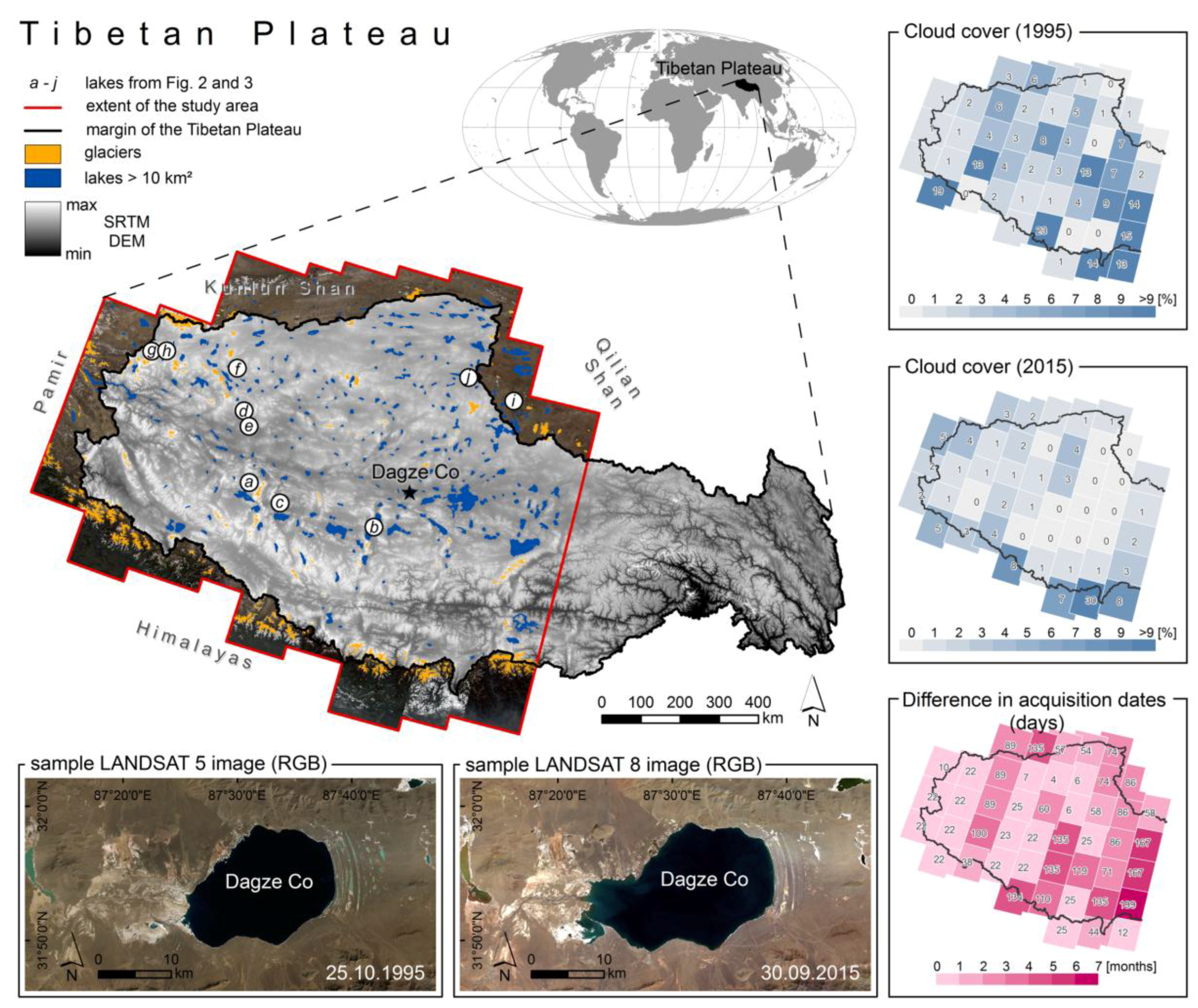
3. Study Area and Data

Our study covered nearly 1,187,000 km², the greater part of the Tibetan Plateau (Figure 1), where lakes mostly formed in tectonic depressions, or behind glaciers and sediments. The lakes have different colours due to sediment concentrations, mineral content (salinity), water depths, aquatic vegetation, and seasonal ice cover (Figure 2). We excluded from our analysis the southeastern Tibetan Plateau because few cloud-free LANDSAT images were available for this area. We analysed 47 LANDSAT 5 images taken in 1995 and 47 LANDSAT 8 images taken in 2015. The size of the study area and the different weather conditions captured on these images required that we analyse different days of the year (i.e., 25 April–17 December 1995, and 8 June–22 November 2015). High-quality images were few for 1995, so we included 22 images from 1994 and four images from 1996. To avoid bias due to seasonal lake-level changes we selected, whenever possible, image pairs that were less than three months apart (Figure 1); for most of the study area, we obtained 36 out of 47 pairs. We selected only images with negligible cloud cover (Figure 1), and atmospheric and sun-angle correction provided by the U.S. Geological Survey (http://espa.cr.usgs.gov/). We used top-of-atmosphere (TOA) reflectance bands instead of at-sensor spectral radiance (SR) because the cosine effect of different solar zenith angles linked to different acquisition times was already removed [31]. TOA reflectance compensates for different values of exoatmospheric solar irradiance arising from spectral band differences; TOA data also account for the varying distance between the Earth and the Sun [31]. To distinguish frozen lakes from glaciers and mountain shadows, we used the SRTM DEM version 4 [56] as a supporting layer in the OBIA, generating a local slope map from the maximum elevation change between pixels in a 3 × 3 neighbourhood.

4. Methods

We developed an algorithm for mapping lakes with seasonal ice cover, combining a water index with digital elevation models using OBIA principles. Our algorithm is insensitive to the physical state of water and allows us to distinguish between frozen lakes and glaciers. We estimated the accuracy of our automatic classification for two time slice datasets for the Tibetan Plateau collected in 1995 and 2015 using a confusion matrix. Furthermore, we tested the transferability of our approach to areas with different environmental conditions. In addition, we verified changes in lake size and general trends over the last 20 years.

An OBIA approach allows the classification of objects from images, by combining spectral properties of pixels and analysing the spatial relation between them. The principle in using this approach is to classify objects that are not uniform across a large area, and to reduce randomly distributed noise that occurs when using pixel-based classification algorithms. The first step in OBIA is segmentation, where pixels are merged into bigger homogenous objects. In the next step, it is possible to build assumptions based on segments’ spectral values. Here, algorithms defining their shape, geometry, spatial position, and connections to the neighbouring segments, are considered an advantage over other classifiers. In OBIA, it is also possible to combine layers of different types of data, such as satellite images and DEM, to extract objects of interest. We chose this approach because attempts to classifying water boundaries based on colour alone have had limited success. From the broad range of available normalised water indices, we selected the MNDWI [27], as it produces the smallest differences between water, snow, and ice, compared to other indices. This allowed us to more easily combine the ‘frozen’ and ‘non-frozen’ parts of a single lake together, while maintaining a stable threshold [43]. We also tested the applicability and the performance of our OBIA workflow for three recently proposed non-normalised water indices: the automated water extraction indices AWEI_nsh and AWEI_sh [44], and the water index WI [45] (Figure 3). For each of these indices, water areas should have positive values, and all other surfaces should have negative values. Glaciers and mountain shadows also have positive values, however, making the classification of lakes in mountainous and glaciered areas like the Tibetan Plateau more difficult.

We generated mosaics from all images for 1995 and 2015 via the Mosaic to New Raster method available in ArcGIS 10.3 software. To speed up the OBIA process, we stretched the MNDWI, AWEI, and WI values into a 0–255 scale (Figure 4b), converting them to 8-bit unsigned integer rasters. We then used a multiresolution segmentation algorithm [57] (Figure 4c) on the MNDWI, AWEI, and WI values. We segmented each index separately, but omitted information on local slope, as the underlying SRTM data were obtained in February 2000, and may thus have biased the segmentation. We also avoided automatic scale selection methods, such as scale-parameter estimation [58] or plateau objective functions [59], as they turned out to be mostly redundant and time consuming. For example, applying the segmentation algorithm to a single LANDSAT image without automatic scale selection using an Intel Core i7-4600U processor with 16GB RAM memory took less than five minutes, whereas using scale-parameter estimation for the same task took more than one hour, partly because some of the segmentation process produced redundant data. The distribution of index values for water bodies (Figure 4b) is more homogenous than those of other types of land cover [24]. The segments for water areas are therefore mostly larger and more compact than for the surrounding landscapes. The multiresolution segmentation algorithm uses three parameters—‘scale’, ‘shape’, and ‘compactness’—which control segment size, roundness, and the degree of homogeneity of values inside the segments, respectively. The crucial point in our OBIA approach was to select an appropriate segment size so that it remained below the smallest lake to be analysed, while remaining large enough to warrant feasible computing times. We selected a scale of 100, shape of 0.1, and a compactness of 0.7 (Figure 4c and Figure 5), after running tests with different parameter combinations, and observing that high values of ‘shape’ and low values of ‘compactness’ performed poorly in classifying water bodies.

We then used the thresholding of the water indices to classify segments as either ‘water’ or ‘other’ (Figure 4d). Due to the different histogram ranges of MNDWI, AWEI_nsh, AWEI_sh, and WI, we developed four individual workflows with different thresholds. First, we applied higher thresholds (MNDWI > 180) to find areas clearly representing water, then incrementally lowered the thresholds (MNDWI > 160) in an infinite loop, adding more neighbourhood assumptions regarding sharing the boundary with segments already classified as water (relative border to water >0.25) and with slopes ≤ 0.5°. The lowest threshold of MNDWI we applied was >150, with a stricter assumption regarding the segment borders; a threshold of >0.4 helped to assign additional water areas, especially those along lake shores or covered by cloud. To distinguish lakes from rivers, we further used the asymmetry of segments and their relation to neighbouring segments. We used the Asymmetry function in the eCognition 9.1 software, defined as the segment length relative to a regular polygon drawn around the segment; asymmetry can range from 0 to 1, with higher values expressing more asymmetric segments. We found that rivers can be separated from lakes for an Asymmetry > 0.85, a relative border to other water segments <0.15, and a boundary shared by a single water segment at the most. Many glaciers on the Tibetan Plateau have MNDWI, AWEI, and WI values similar to those of lakes, so that a pure OBIA-based classification based on a water index produced many misclassifications. We therefore used a local slope map generated from SRTM DEM as a supporting layer; as most glaciers occupy areas with slopes >2° (Figure 4e), we reclassified all segments accordingly. In a neighbourhood analysis, we corrected segments that were misclassified as glaciers (Figure 4f). We reclassified all segments from the glacier class with relative borders to water bodies and glaciers of >0.4 and ≤0.1, respectively, as water. Accordingly, we reclassified water class segments with relative borders to glaciers and water bodies of ≥0.4 and <0.1, respectively, and with a mean slope >0.5°, as glaciers, merging neighbouring segments assigned to the same class (Figure 4g).

To reduce errors arising from the resolution of satellite images and the DEM, we focused on lakes that were >10 km² in size in 2015 (see Section 5.1), and exported these as vector polygons for further quality assessment (Figure 4h). The whole procedure for automatic lake detection using an Intel Core i7-4600U processor with 16GB RAM memory took us ~15 min for each processed tile (we had 16 tiles in total), where each individual raster tile contained 12.156 columns and 10.405 rows (~113,835 km²). We used the lake polygons to generate reference data, visually checking the accuracy of each single lake boundary based on natural colour mosaics, and manually improving the automatically-extracted lakes where necessary. Manual digitising of each lake was necessary because the lakes on the Tibetan Plateau change their size seasonally and in the long term, resulting in no available accurate reference data. We applied the same digitisation scheme and rules for all manually-generated lake polygons.

We digitised the reference data by photographic interpretation of LANDSAT images in 2D in ArcMap 10.3 at scales between 1:5000 and 1:20,000, depending on the complexity of the lake shores. We selected this scale range by taking into account the minimum mapping unit of our images, which was 30 × 30 m. We also checked whether lakes were overlooked by the automatic classification or other objects were falsely assigned as lakes. Several lakes, had diffuse boundaries due to lake salinity, clouds, or mountain shadows, which hindered correct interpretation of images. In such cases, we used water index maps and images with higher resolution, available at ArcGIS online, as supporting layers to delineate the lake boundary. In total, we generated 323 reference lakes for each time slice. We used these reference data to estimate the accuracy of the classification (

Table 2. Summary of performance metrics of the classification of lakes on the Tibetan Plateau.

Performance Metrics
Type I error	FP/(TP + FP)
Type II error	FN/(FN + TN)
Total error	(FP + FN)/(TP + FP + FN + TN)
Overall accuracy	(TP + TN)/(TP + FP + FN + TN)
Producer’s accuracy	TP/(TP + FP)
User’s accuracy	TP/(TP + FN)
Cohen’s kappa	(po − pe)/(1 − pe)
F-score	2TP/(2TP + FP + FN)
Root mean square error	$\sqrt{\frac{1}{N}{{\displaystyle \sum }}_{i=1}^N{\left(x_i-{\widehat{x}}_i\right)}^2}$
Mean absolute error	$\frac{1}{N}{{\displaystyle \sum }}_{i=1}^N\left|x_i-{\widehat{x}}_i\right|$
Bias (Mean error)	$\frac{1}{N}{{\displaystyle \sum }}_{i=1}^N\left(x_i-{\widehat{x}}_i\right)$

TP—true positive; FP—false positive; FN—false negative; TN—true negative; p_o—relative observed agreement among rates; p_e—hypothetical probability of chance agreement; $x_i$—predicted value; ${\widehat{x}}_i$—observed value; N—number of observations.

) in terms of type I error, type II error, total error [60], overall accuracy, producer’s accuracy, user’s accuracy [61], Cohen’s kappa [62], and F-score measures. In addition, we estimated root mean square error, mean absolute error, and mean error (bias) (Table 2). The most significant measure is user’s accuracy, because it describes whether the automatically extracted lakes were captured in the reference data.

5. Results

Our classification of Tibetan lakes detected 323 lakes with areas of >10 km² in the study area in 2015, with a total area of 31,258 km², or 2.6% of the study area. Twenty years earlier, the same lakes covered only 24,892 km², meaning that their total area grew by ~26% (see detailed data online at http://arcg.is/1r8Mj4a).

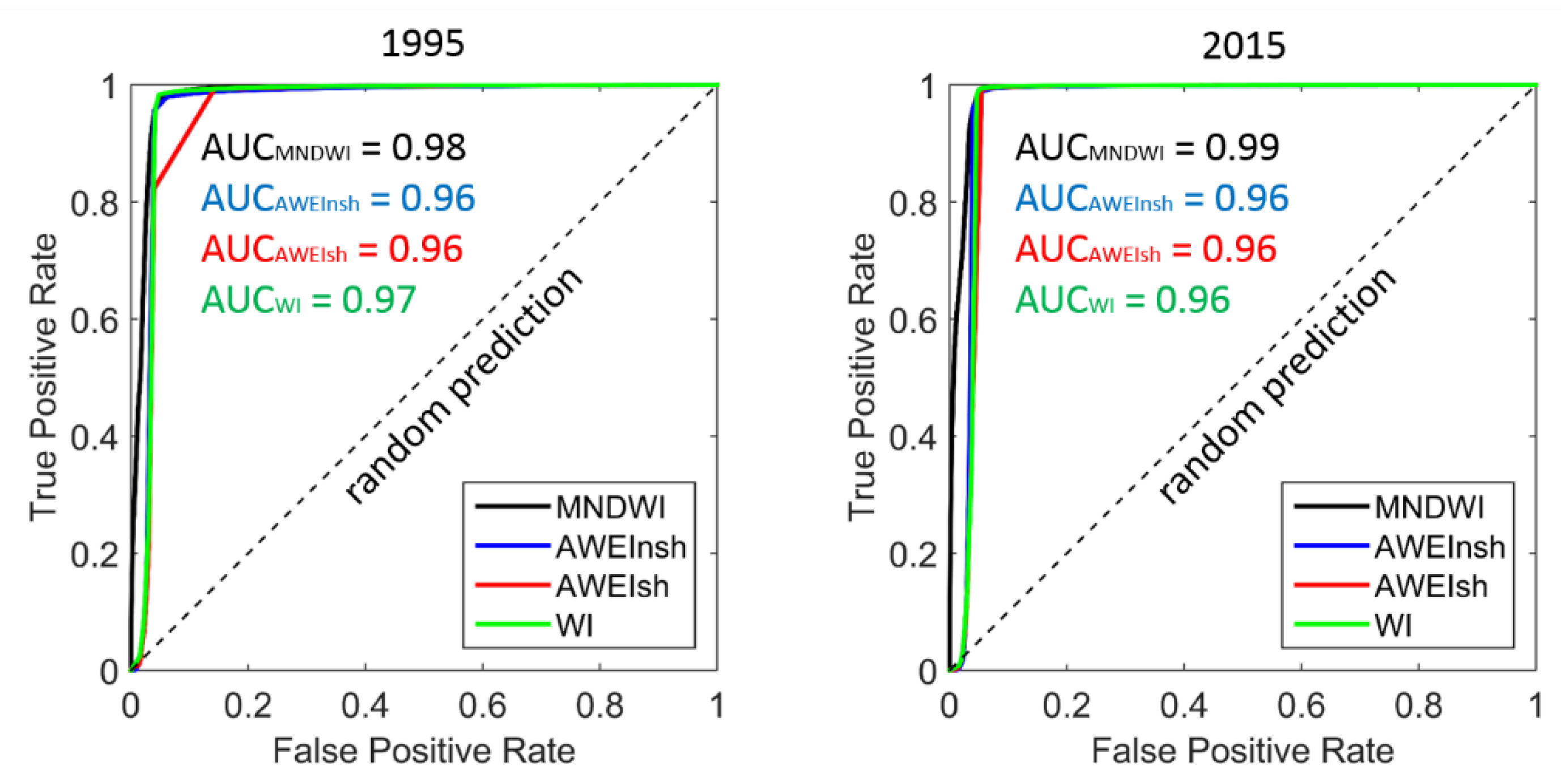
5.1. Accuracy of Extracted Lakes

We selected a minimum lake area of 10 km², given the 30-m resolution of the satellite images and to minimise the influence of mixed pixels from low-resolution images. The proportion of mixed pixels to total lake pixels increases with decreasing lake area (Figure 6). For lakes <10 km², this proportion is >0.2, whereas for lakes >50 km² it is <0.07. Estimating the accuracy of lakes with high percentages of mixed pixels may therefore misrepresent the accuracy of the method. We compared the classified lake boundaries with the manually generated reference data and computed several performance metrics for the entire study area (

Table 3. Performance metrics for OBIA-based extraction of lakes on the Tibetan Plateau with MNDWI, WI, AWEI_nsh, and AWEI_sh for 1995 and 2015.

Performance Metric	1995				2015
	MNDWI	WI	AWEInsh	AWEIsh	MNDWI	WI	AWEInsh	AWEIsh
Type I	0.0134	0.0089	0.0234	0.0140	0.0169	0.0081	0.0337	0.0143
Type II	0.0003	0.0016	0.0005	0.0022	0.0005	0.0018	0.0007	0.0016
Total	0.0006	0.0018	0.0010	0.0024	0.0010	0.0020	0.0016	0.0020
O. Acc.	0.9994	0.9982	0.9990	0.9976	0.9990	0.9980	0.9984	0.9980
P. Acc.	0.9866	0.9911	0.9766	0.9860	0.9831	0.9919	0.9663	0.9857
U. Acc.	0.9850	0.9292	0.9778	0.9073	0.9808	0.9376	0.9732	0.9428
Kappa	0.9855	0.9583	0.9767	0.9438	0.9815	0.9630	0.9690	0.9628
F-score	0.9858	0.9592	0.9772	0.9450	0.9819	0.9640	0.9698	0.9638
RMSE	0.0244	0.0420	0.0309	0.0490	0.0309	0.0442	0.0398	0.0442
MAE	0.0005	0.0018	0.0010	0.0024	0.0010	0.0020	0.0016	0.0020
ME	−0.0003	−0.0014	0.0003	−0.0018	−0.0001	−0.0015	0.0002	−0.0012

Type I error (Type I); Type II error (Type II); Total error (Total); Overall accuracy (O. Acc.); Producer’s accuracy (P. Acc.); User’s accuracy (U. Acc.); Cohen’s kappa (Kappa); Root mean square error (RMSE); Mean absolute error (MAE); Mean error (ME).

).

Our OBIA method for extracting lakes >10 km² had an overall accuracy of 0.99, and the producer’s and user’s accuracy, Cohen’s kappa, and the F-score for both time slices were >0.98 when using the MNDWI (Table 3). The performance with AWEI_nsh, AWEI_sh and WI was slightly lower, albeit >0.94, with the exception of the user’s accuracy for WI of ~0.92. The accuracy in classifying lakes with respect to their physical states of water (frozen, partly frozen, and unfrozen) was similar. All lakes, irrespective of ice cover, were detected with very high producer’s accuracy (Figure 7). The MNWDI achieved the highest accuracy and the lowest root mean square error, mean absolute error, and mean error; we checked the performance of standalone water indices in extracting lakes >10 km² (Figure 8), and found that the area under the curve (AUC) of MNWDI exceeded those of the AWEI and WI indices.

Visual cross checks revealed that using the AWEI_sh in our OBIA approach misclassified many land areas as lakes, especially by falsely assigning border segments adjacent to lakes (Figure 9, Table 3). The AWEI_nsh appeared to be the least useful for selecting thresholds between water and non-water pixels (Figure 9). Histograms showed that the zero threshold was more reliable to use on MNDWI than any other water index. Most misclassified areas were along the border of lakes, particularly irregular shorelines; river deltas were also often represented by single segments in our method. Clouds also caused some misclassification of lakes (Figure 9), whereas glaciers were a lesser problem. In some cases, small islands in the lakes were also misclassified.

We note that seasonal lake ice had little influence on our data; however, with our OBIA approach, lakes were mostly classified correctly regardless. We studied Siling Co, in detail, which is the largest lake in our study area (though not on the entire Tibetan Plateau). We selected additional images for the two time slices, covering more seasonal variations in lake ice and snow cover on shorelines. To this end, we used the OBIA classification with the MNDWI without changing any parameter in the workflow. We found our method to be robust throughout and capable of detecting lakes with high accuracy (Figure 10). Misclassification occurred only in an image obtained on 2 December 1994, in which shores were covered by snow, violating the assumptions of our OBIA approach designed exclusively for snow-free images.

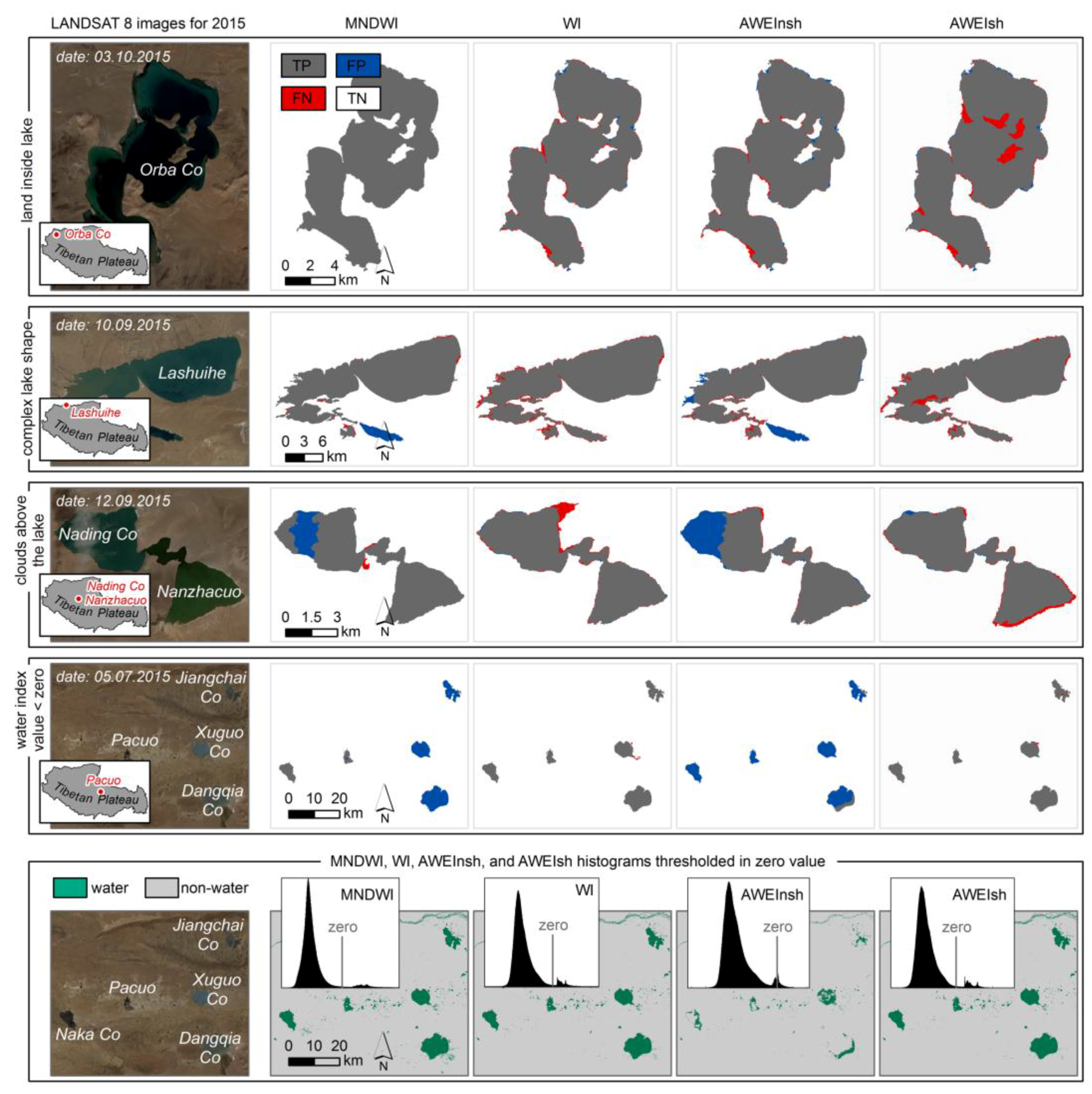
5.2. Sources of Error in the Analyses

Although our classification has very high accuracy, we have highlighted several sources of error unrelated to the algorithm but nevertheless influencing our classification. The first source of error arose from splitting the data into smaller tiles. To make our analysis feasible, we had to separate the study area into 16 square tiles with two pixels of overlap between neighbouring tiles. This led to misclassifying small parts of lakes along the borders of the tiles.

Another source of error concerned reference data that solely relied on LANDSAT images. The 30-m resolution of images made it difficult to delineate some of the blurrier lake images. The roundness of the lakes also played a role, as rounded shapes with a lower perimeter-area ratio are easier to digitise. This ratio translated into the number of pixels along lake borders for which correct classification was difficult. Another important point is that manually-generated reference data are always prone to operator bias, as different people are likely to map the same lakes with minor differences. Such differences may produce fake changes in lake areas, and therefore we treated any lake-area changes of <1 km² as potentially suspicious.

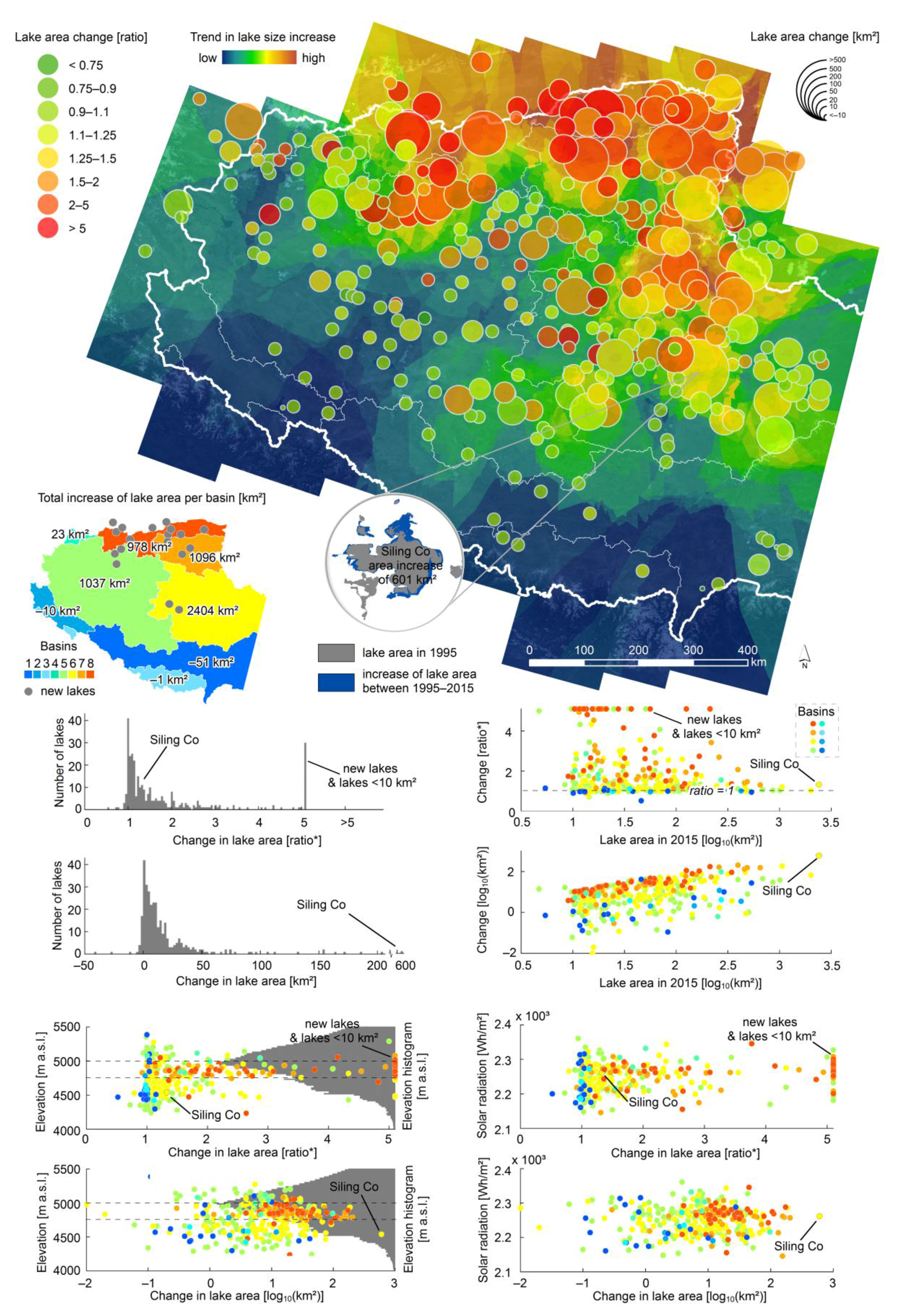
5.3. Lake-Area Changes (1995–2015)

Our analysis showed that the total area of lakes >10 km² on the Tibetan Plateau increased by 6366 km². Out of 323 lakes, 25 increased their area by >50 km², eleven lakes grew by >100 km², and one lake by >500 km². These changes were not evenly spread throughout the study area. The highest relative increase occurred in the northern part of the Tibetan Plateau, where most lakes are concentrated (Figure 11); these grew mostly by between 100% and 200%, and up to 50 km² in absolute area (Figure 11). The highest increase in total lake area (2404 km²) occurred in internal basin ‘6’ on the northeastern part of the plateau, where 108 lakes were detected (Figure 11). In basin ‘5’, which has a similar number of lakes (112), the total lake area increased by 1037 km². Most lakes that underwent moderate changes (<10 km²) are in the southwestern Tibetan Plateau, mainly along the Himalayas and adjacent mountain belts (see detailed data online at https://uni-potsdam.maps.arcgis.com/apps/webappviewer/index.html?id=3595915b0af244c89750823133a9e165). Between 1995 and 2015, eighteen new lakes >1 km² formed mostly in the northeastern part of the plateau, at elevations between 4700 and 5000 m a.s.l., slightly below the most dominant elevation (Figure 11). This narrow elevation band also featured the greatest increase in lake size, whereas most lakes with lesser changes lie at lower elevation. We notice a weak correlation of lake growth with incoming solar radiation, especially for basins ‘7’ and ‘8’ (Figure 11).

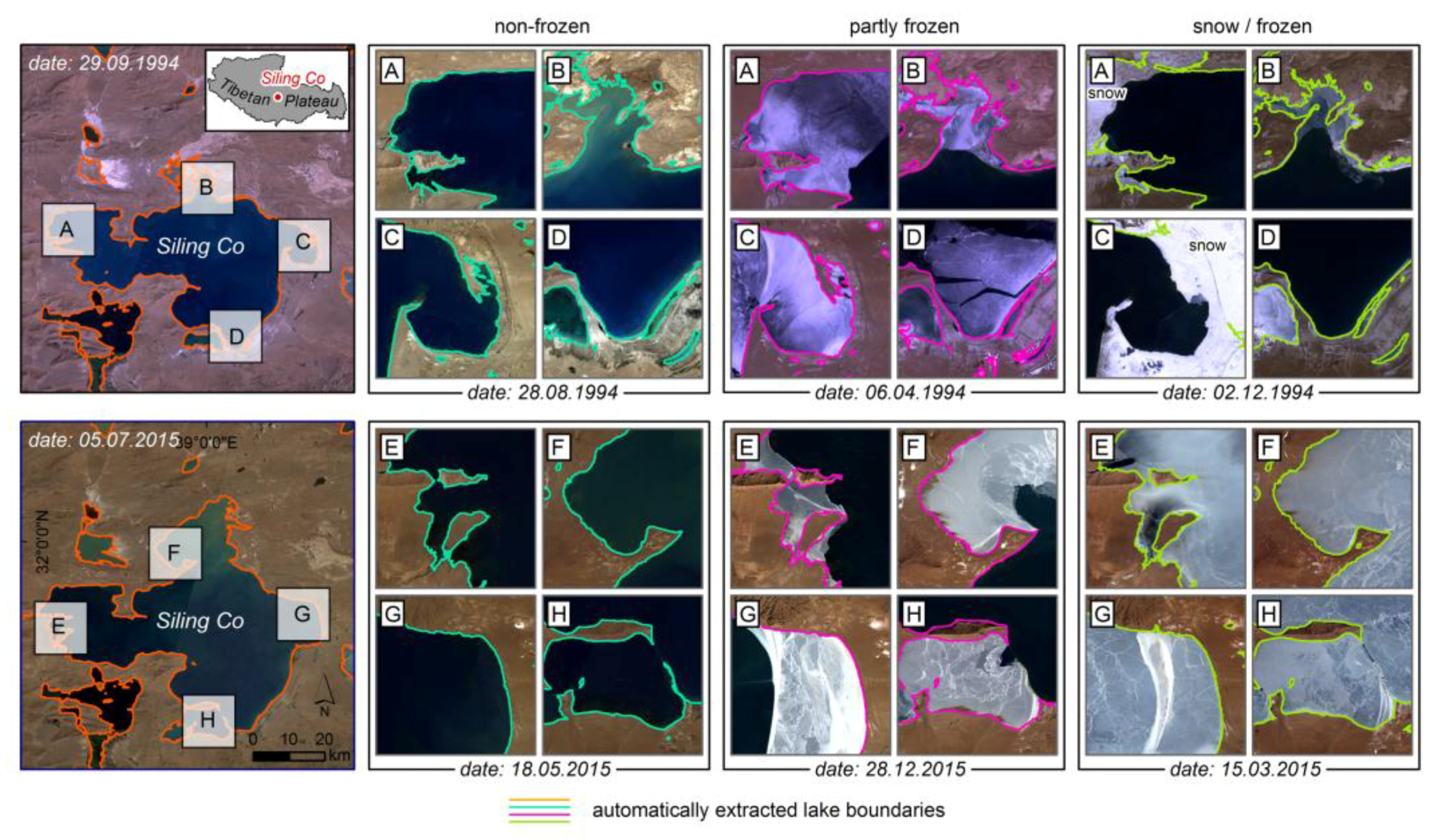
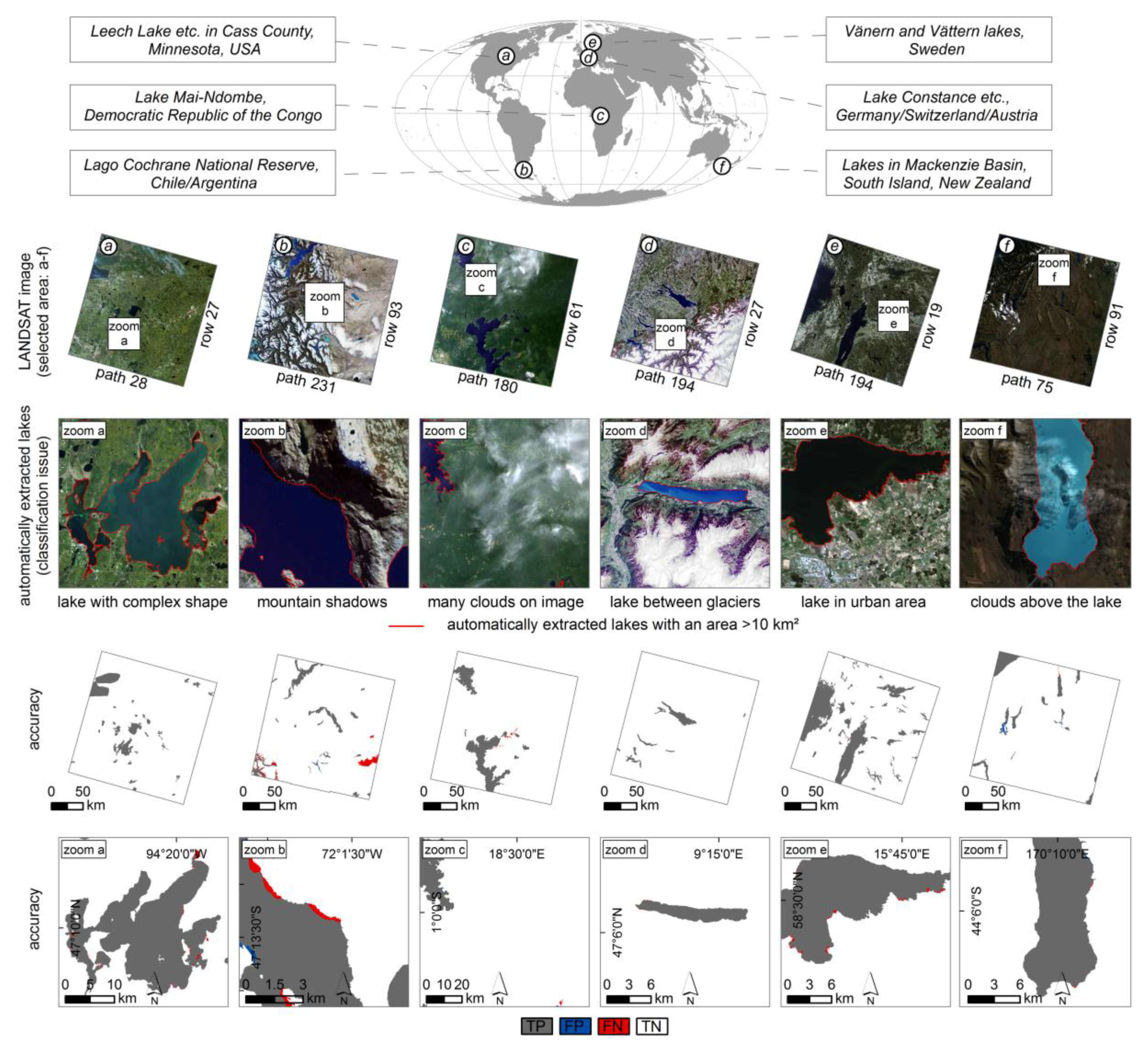
5.4. Transferability of OBIA Approach

We tested the global transferability of our method for extracting lakes with the MNDWI, as this index achieved the highest accuracy. We selected six LANDSAT 8 images capturing areas with numerous lakes on five continents, representing environments greatly different to that of the Tibetan Plateau (Figure 12,

Table 4. Characteristics of test sites across the world used to verify the transferability of our OBIA method for lake classification (see Figure 12 for locations).

TS	Continent (Country)	Landscape Type	Extracted Lakes	Date	TA
a	North America (USA)	Flat area	Leech Lake, etc. in Cass County, Minnesota	29.09.2015	2156.28
b	South America (Chile/Argentina)	Mountains	Lakes in Lago Cochrane National Reserve	01.04.2014	1518.87
c	Africa (Democratic Republic of the Congo)	Flat forested area	Mai-Ndombe Lake, etc.	12.01.2016	2812.52
d	Europe (Germany/Switzerland/Austria)	Mountains with glaciers	Constance Lake, etc.	22.05.2016	802.76
e	Europe (Sweden)	Lakeland—flat postglacial area	Vänern and Vättern Lakes, etc.	09.05.2016	5848.82
f	Australia (New Zealand)	Hilly region	Lakes in Mackenzie Basin	17.03.2016	1696.70

TS (test site); Date (Image acquisition date [day.month.year]); TA (Total area [km²] of lakes >10 km² on image).

).

We maintained our OBIA workflow for these selected areas without changing any parameters, and found that nearly all classified test areas yielded overall, producer’s, and user’s accuracies of >0.95, with a Cohen’s kappa and F-score of >0.96, with low root mean square errors, mean absolute errors, and mean errors (

Table 5. Performance metrics for OBIA-based lake extraction using MNDWI for lakes in different test areas across the world (see Figure 12 for locations).

Performance Metrics	Test Area
	a	b	c	d	e	f
Type I error	0.0022	0.0216	0.0021	0.0050	0.0025	0.0471
Type II error	0.0004	0.0120	0.0014	0.0001	0.0012	0.0005
Total error	0.0005	0.0124	0.0014	0.0002	0.0014	0.0027
Overall accuracy	0.9995	0.9876	0.9986	0.9998	0.9986	0.9973
Producer’s accuracy	0.9978	0.9784	0.9979	0.9950	0.9975	0.9529
User’s accuracy	0.9940	0.7825	0.9835	0.9948	0.9939	0.9899
Cohen’s kappa	0.9956	0.8631	0.9898	0.9948	0.9949	0.9697
F-score	0.9959	0.8695	0.9906	0.9949	0.9957	0.9711
Root mean square error	0.0220	0.1113	0.0381	0.0149	0.0369	0.0515
Mean absolute error	0.0005	0.0124	0.0014	0.0002	0.0014	0.0027
Mean error	−0.0002	−0.0106	−0.0011	−0.0001	−0.0006	0.0017

). For one test area, the lakes in Lago Cochrane National Reserve, Chile, the performance metrics were much lower, mainly because the algorithm misclassified a single large river delta (Figure 12b). Visual checks indicated that flat and hilly regions allow for better delineation of lake boundaries than high mountains. Shadows were correctly distinguished from lakes; however, where shadows overlapped with lakes, misclassifications arose. Small and thin clouds were usually correctly distinguished from lakes (Figure 12f); however, thicker clouds increased misclassification (Figure 9). Overall, our method performed well for nearly all landscape types, including low-gradient environments without glaciers (Figure 12a) and alpine environment with glaciers (Figure 12d, Table 5).

6. Discussion

In the second part of the 20th century, 82% of the Tibetan Plateau glaciers retreated; if this trend continues, two-thirds of the current Tibetan Plateau glaciers could be gone in the coming centuries [1]. Changes in evaporation may significantly increase this trend, supplying water to lakes and enhancing their growth. Systematically monitoring lake areas therefore supports estimates of the rates of change. Our comparative analysis confirms previous findings that have reported that expanding lakes are not spread uniformly across the Tibetan Plateau [6,19,21], but are instead focused in the northeastern part of the Plateau. Compared to the distribution of glaciers (Figure 1), we found that lakes grew by the smallest amount where glaciers in the Himalayan Mountains Range are most numerous. This may be due to the temperature increase, which may promote stronger evaporation [25].

Accurate automated mapping of lake boundaries may aid regional studies of the hydrological balance of tens to thousands of lakes. Our OBIA based approach provides a tool that allows, in a short time and an easy way, to delineate the shorelines of large lakes, thus assisting the monitoring of regional changes in lake size, both seasonal and in the long term. The performance of our automatic classification tested on the Tibetan Plateau is surprisingly high. Tests of our method on lakes in other environments, without changing any parameters, were similarly successful, and most lakes were correctly detected with only minor misclassification at the boundaries of lakes, especially where shorelines were complex. This high accuracy largely draws from using a water index in an OBIA context. The water index we used, the MNDWI, is generally highly accurate; however, misclassifying glaciers, shadows, and clouds, as well as its varying threshold for separating ‘water’ from other land-cover types—which should be around zero value—makes it difficult to transfer the method to areas outside of the training area. We implemented water index thresholding in the OBIA using few thresholds, which more correctly detected the lakes’ boundaries than did single thresholding. Applying neighbourhood assumptions for every segment allowed us to distinguish lakes from other objects falsely assigned by the water index. By using a multiresolution segmentation algorithm, we reduced unwanted salt-and-pepper noise that is a characteristic of simple water index thresholding. The OBIA rule set relied on relations between the segments and their spatial location, allowing us to more realistically separate lakes from other bjects with similar water index values. The OBIA protocol found segments that were incorrectloy classified by the MNDWI thresholding due to their low values caused by clouds above the lakes, MNDWI values that were too low, or shadows, and subsequently re-classified them as lakes. The topographic slope information excludes glaciers and other falsely included objects. Although our method is designed for lakes >10 km², it is capable of extracting numerous smaller lakes accurately; however, we omitted some small lakes (<1 km²) owing to the choice of ‘scale’ parameter. For detecting lakes <10 km² more correctly, we recommend decreasing the ‘size’ of segments. The smallest correctly-identified lake for the 1995 images had an area of 0.0135 km² (15 pixels). The correctness of its predicted boundaries is difficult to check, however, given the 30-m data resolution.

Mixed pixels along lake shores remain a major challenge for classification. We have shown that they can form a large proportion of the classified lake area, especially for small lakes and low-resolution images, thus increasing the cost of classifying them compared to large lakes. We suggest that this proportion should not exceed 10% of the area of the smallest object of interest. This is why we focused only on lakes >10 km², as for most of these lakes the mixed pixels ratio was <10% (Figure 6).

We found that MNDWI accurately indicated of water areas, detecting nearly all lakes in our study area. Compared to several other water indices, the MNDWI ROC curve indicated the best performance in detecting lakes >10 km²; additionally its derivation is physically more intuitive than those for the WI and AWEI. In computing the MNDWI, one may neglect erroneous pixels in the input bands, because for such errors the absolute value of MNDWI will be >1, thus enabling fast and easy quality checks. For computing the AWEI and WI, this issue remained pending; therefore, one must check all input bands carefully and exclude erroneous values from the bands separately. The MNWDI is a normalised metric, and therefore it is easier to manipulate, contrast, and stretch the data as desired, while the range of values remains the same with respect to SR or TOA data, making it possible to use the same threshold independently of the input data.

Combining optical images with elevation models enabled us to build more sophisticated assumptions in OBIA and separate lakes from glaciers, which have similar spectral properties on LANDSAT images. A slope map derived from DEM gives adequate information on the differences between these two landforms. Lakes have a slope of approximately zero, whereas the slope for glaciers is mostly larger. Although the slope of some lake shores may be similar to that of glaciers, the use of common boundaries with other flatter lake segments promotes a correct assignment to the lake class. In very steep terrain, lake-shore pixels can have spuriously high slopes as an artefact of including nearby hillslopes. Using a more accurate DEM may allow us to achieve better results, especially if the DEM data were gathered shortly before or after the time slice of interest. We used a DEM from 2000 to analyse lakes in 1995 and 2015, so that five and 15 years of geomorphic change could have affected our elevation data. LANDSAT images are available for the entire globe; however, SRTM data are only available between 56° S and 60° N. The lack of more digital topographic data for areas with higher altitude therefore curtails our method, particularly in Arctic regions featuring thousands of glacial and periglacial lakes. In such cases, however, a new global 0.4 arc second (~12m) DEM gathered by the TerraSAR-X-Add-on for Digital Elevation Measurements (TanDEM-X) mission (https://tandemx-science.dlr.de/) may open new doors.

We also recall that, in snow-covered areas, the multiresolution segmentation algorithm is unable to properly delineate lake boundaries using a water index, so we recommend using our method only for images without snow cover. Using a metric of the spread of water-index values, such as their standard deviation, may help to distinguish water from snow. Similarly, clouds remain an issue in detecting lake boundaries. The fraction of cloud cover provided with LANDSAT images may be insufficient because even an image with low cloud cover may introduce classification errors, where clouds obscuring parts of lakes can be crucial. Visual checks of images remain indispensable. We recommend tools such as the LAND Viewer (http://lv.eosda.com), which enables verification of the RGB and different band compositions of LANDSAT-8 and SENTINEL-2 images in relation to date, percentage of cloud, and sun angle in detail before downloading.

Our method fills in a gap in classifying lakes prone to seasonal ice cover, as such lakes are notoriously difficult to detect automatically. Our automatic and fast classification allows the mapping of water bodies, irrespective of landscape type, with an accuracy similar to those of previous approaches [48,49,63]. The added value of our algorithm is that it detects lakes regardless of whether they are partly or completely frozen. We therefore believe that our OBIA algorithm has great potential for tracking in detail not only long-term changes, but also seasonal variations in lake areas, especially given the increasing access to free high-resolution satellite images, such as those from the SENTINEL sensor, which revisits a given area every five days.

7. Conclusions

We have proposed an approach for automatically detecting large lakes prone to seasonal ice cover. We developed our method for the Tibetan Plateau, where such ice cover and surrounding glaciers make the use of various remote-sensing-based water indices problematic. Our method is insensitive in this regard and distinguishes with high estimated accuracy between lakes, glaciers, and shadows, giving the opportunity to track annual and seasonal changes of mountain lakes, especially those surrounded by many glaciers. Our approach combines a satellite-image-derived water index, OBIA, and a DEM-derived slope map to automatically extract lakes. The method can be applied in areas where acquiring images in ice-free seasons is difficult. Testing of our method on LANDSAT images for two time slices (1995 and 2015) showed that lakes on the Tibetan Plateau grew ~26% in total, and that the changes were not evenly spread through the whole tested area. The largest increase occurred in the northeast, whereas the southwestern Tibetan Plateau saw the largest decrease. Further tests of our method in areas abundant in lakes throughout the world showed that our approach may be general and flexible enough for regional, if not global, monitoring of lake changes.

References

1. Qiu, J. The Third Pole. Nature 2008, 454, 393–396. [Google Scholar] [CrossRef] [PubMed]
2. Song, C.; Huang, B.; Ke, L.; Richards, K.S. Remote sensing of alpine lake water environment changes on the Tibetan Plateau and surroundings: A review. ISPRS J. Photogramm. Remote Sens. 2014, 92, 26–37. [Google Scholar] [CrossRef]
3. Wang, C. A remote sensing perspective of alpine grasslands on the Tibetan Plateau: Better or worse under ‘Tibet Warming’? Remote Sens. Appl. Soc. Environ. 2016, 3, 36–44. [Google Scholar] [CrossRef]
4. Liu, X.; Chen, B. Climatic warming in the Tibetan Plateau during recent decades. Int. J. Climatol. 2000, 20, 1729–1742. [Google Scholar] [CrossRef]
5. Immerzeel, W.W.; van Beek, L.P.H.; Bierkens, M.F.P. Climate change will affect the Asian Water Towers. Science 2010, 328, 1382–1385. [Google Scholar] [CrossRef] [PubMed]
6. Song, C.; Huang, B.; Ke, L. Modeling and analysis of lake water storage changes on the Tibetan Plateau using multi-mission satellite data. Remote Sens. Environ. 2013, 135, 25–35. [Google Scholar] [CrossRef]
7. Immerzeel, W.W.; Kraaijenbrink, P.D.A.; Shea, J.M.; Shrestha, A.B.; Pellicciotti, F.; Bierkens, M.F.P.; De Jong, S.M. High-resolution monitoring of Himalayan glacier dynamics using unmanned aerial vehicles. Remote Sens. Environ. 2014, 150, 93–103. [Google Scholar] [CrossRef]
8. Yao, T.; Thompson, L.; Yang, W.; Yu, W.; Gao, Y.; Guo, X.; Yang, X.; Duan, K.; Zhao, H.; Xu, B.; et al. Different glacier status with atmospheric circulations in Tibetan Plateau and surroundings. Nat. Clim. Chang. 2012, 2, 663–667. [Google Scholar] [CrossRef]
9. Zhang, Y.; Yao, T.; Ma, Y. Climatic changes have led to significant expansion of endorheic lakes in Xizang (Tibet) since 1995. Sci. Cold Arid Reg. 2011, 3, 463–467. [Google Scholar]
10. Yao, T.; Thompson, L.G.; Mosbrugger, V.; Zhang, F.; Ma, Y.; Luo, T.; Xu, B.; Yang, X.; Tayal, S.; Jilani, R.; et al. Third Pole Environment (TPE). Environ. Dev. 2012, 3, 52–64. [Google Scholar] [CrossRef]
11. Yang, W.; Yao, T.; Xu, B.; Wu, G.; Ma, L.; Xin, X. Quick ice mass loss and abrupt retreat of the maritime glaciers in the Kangri Karpo Mountains, southeast Tibetan Plateau. Chin. Sci. Bull. 2008, 53, 2547–2551. [Google Scholar] [CrossRef]
12. Yang, M.; Nelson, F.E.; Shiklomanov, N.I.; Guo, D.; Wan, G. Permafrost degradation and its environmental effects on the Tibetan Plateau: A review of recent research. Earth-Sci. Rev. 2010, 103, 31–44. [Google Scholar] [CrossRef]
13. Yang, X.; Lu, X. Drastic change in China’s lakes and reservoirs over the past decades. Sci. Rep. 2014, 4, 1–10. [Google Scholar] [CrossRef] [PubMed]
14. Shao, Z.G.; Zhu, D.G.; Meng, X.G.; Zheng, D.X.; Qiao, Z.J.; Bin Yang, C.; Han, J.E.; Yu, J.; Meng, Q.W.; Lü, R.P. Characteristics of the change of major lakes on the Qinghai-Tibet Plateau in the last 25 years. Geol. Bull. China 2007, 26, 1633–1645. [Google Scholar] [CrossRef]
15. Zhu, L.P.; Xie, M.P.; Wu, Y.H. Quantitative analysis of lake area variations and the influence factors from 1971 to 2004 in the Nam Co basin of the Tibetan Plateau. Chin. Sci. Bull. 2010, 55, 1294–1303. [Google Scholar] [CrossRef]
16. Zhang, G.; Xie, H.; Kang, S.; Yi, D.; Ackley, S.F. Monitoring lake level changes on the Tibetan Plateau using ICESat altimetry data (2003–2009). Remote Sens. Environ. 2011, 115, 1733–1742. [Google Scholar] [CrossRef]
17. Phan, V.H.; Lindenbergh, R.; Menenti, M. ICESat derived elevation changes of Tibetan lakes between 2003 and 2009. Int. J. Appl. Earth Obs. Geoinf. 2012, 17, 12–22. [Google Scholar] [CrossRef]
18. Ouma, Y.O.; Tateishi, R. A water index for rapid mapping of shoreline changes of five East African Rift Valley lakes: An empirical analysis using Landsat TM and ETM+ data. Int. J. Remote Sens. 2006, 27, 3153–3181. [Google Scholar] [CrossRef]
19. Song, C.; Huang, B.; Ke, L.; Richards, K.S. Seasonal and abrupt changes in the water level of closed lakes on the Tibetan Plateau and implications for climate impacts. J. Hydrol. 2014, 514, 131–144. [Google Scholar] [CrossRef]
20. Ma, R.; Duan, H.; Hu, C.; Feng, X.; Li, A.; Ju, W.; Jiang, J.; Yang, G. A half-century of changes in China’s lakes: Global warming or human influence? Geophys. Res. Lett. 2010, 37, 2–7. [Google Scholar] [CrossRef]
21. Fang, Y.; Cheng, W.; Zhang, Y.; Wang, N.; Zhao, S.; Zhou, C.; Chen, X.; Bao, A. Changes in inland lakes on the Tibetan Plateau over the past 40 years. J. Geogr. Sci. 2016, 26, 415–438. [Google Scholar] [CrossRef]
22. Liu, J.; Kang, S.; Gong, T.; Lu, A. Growth of a high-elevation large inland lake, associated with climate change and permafrost degradation in Tibet. Hydrol. Earth Syst. Sci. 2010, 14, 481–489. [Google Scholar] [CrossRef]
23. Lei, Y.; Yao, T.; Bird, B.W.; Yang, K.; Zhai, J.; Sheng, Y. Coherent lake growth on the central Tibetan Plateau since the 1970s: Characterization and attribution. J. Hydrol. 2013, 483, 61–67. [Google Scholar] [CrossRef]
24. Li, J.; Sheng, Y.; Luo, J. Automatic extraction of Himalayan glacial lakes with remote sensing. J. Remote Sens. 2011, 15, 29–43. [Google Scholar]
25. Wang, X.; Gong, P.; Zhao, Y.; Xu, Y.; Cheng, X.; Niu, Z.; Luo, Z.; Huang, H.; Sun, F.; Li, X. Water-level changes in China’s large lakes determined from ICESat/GLAS data. Remote Sens. Environ. 2013, 132, 131–144. [Google Scholar] [CrossRef]
26. Blaschke, T. Object based image analysis for remote sensing. ISPRS J. Photogramm. Remote Sens. 2010, 65, 2–16. [Google Scholar] [CrossRef]
27. Xu, H. Modification of normalised difference water index (NDWI) to enhance open water features in remotely sensed imagery. Int. J. Remote Sens. 2006, 27, 3025–3033. [Google Scholar] [CrossRef]
28. Singh, A. Review Article Digital change detection techniques using remotely-sensed data. Int. J. Remote Sens. 1989, 10, 989–1003. [Google Scholar] [CrossRef]
29. Melesse, A.M.; Weng, Q.; Thenkabail, P.S.; Seney, G.B. Remote sensing sensors and applications in environmental resources mapping and modelling. Sensors 2007, 7, 3209–3241. [Google Scholar] [CrossRef]
30. Arp, C.D.; Jones, B.M.; Lu, Z.; Whitman, M.S. Shifting balance of thermokarst lake ice regimes across the Arctic Coastal Plain of northern Alaska. Geophys. Res. Lett. 2012, 39, 1–5. [Google Scholar] [CrossRef]
31. Chander, G.; Markham, B.L.; Helder, D.L. Summary of current radiometric calibration coefficients for Landsat MSS, TM, ETM+, and EO-1 ALI sensors. Remote Sens. Environ. 2009, 113, 893–903. [Google Scholar] [CrossRef]
32. Frazier, P.S.; Page, K.J. Water body detection and delineation with Landsat TM data. Photogramm. Eng. Remote Sens. 2000, 66, 1461–1467. [Google Scholar]
33. McFeeters, S.K. Using the normalized difference water index (NDWI) within a geographic information system to detect swimming pools for mosquito abatement: A practical approach. Remote Sens. 2013, 5, 3544–3561. [Google Scholar] [CrossRef]
34. Mueller, N.; Lewis, A.; Roberts, D.; Ring, S.; Melrose, R.; Sixsmith, J.; Lymburner, L.; McIntyre, A.; Tan, P.; Curnow, S.; et al. Water observations from space: Mapping surface water from 25 years of Landsat imagery across Australia. Remote Sens. Environ. 2016, 174, 341–352. [Google Scholar] [CrossRef]
35. Yang, K.; Smith, L.C. Supraglacial streams on the Greenland ice sheet delineated from combined spectral-shape information in high-resolution satellite imagery. IEEE Geosci. Remote Sens. Lett. 2013, 10, 801–805. [Google Scholar] [CrossRef]
36. Fitzpatrick, A.A.W.; Hubbard, A.L.; Box, J.E.; Quincey, D.J.; Van As, D.; Mikkelsen, A.P.B.; Doyle, S.H.; Dow, C.F.; Hasholt, B.; Jones, G.A. A decade (2002–2012) of supraglacial lake volume estimates across Russell Glacier, West Greenland. Cryosphere 2014, 8, 107–121. [Google Scholar] [CrossRef]
37. Zhu, W.; Jia, S.; Lv, A. Monitoring the fluctuation of Lake Qinghai using multi-source remote sensing data. Remote Sens. 2014, 6, 10457–10482. [Google Scholar] [CrossRef]
38. Nath, R.K.; Deb, S.K. Water-body area extraction from high resolution satellite images-An Introduction, review, and comparison. Int. J. Image Process. 2010, 3, 353–372. [Google Scholar]
39. Ryu, J.H.; Won, J.S.; Min, K.D. Waterline extraction from Landsat TM data in a tidal flat a case study in Gomso Bay, Korea. Remote Sens. Environ. 2002, 83, 442–456. [Google Scholar] [CrossRef]
40. McFeeters, S.K. The use of the Normalized Difference Water Index (NDWI) in the delineation of open water features. Int. J. Remote Sens. 1996, 17, 1425–1432. [Google Scholar] [CrossRef]
41. Townshend, J.R.G.; Justice, C.O. Analysis of the dynamics of African vegetation using the normalized difference vegetation index. Int. J. Remote Sens. 1986, 7, 1435–1445. [Google Scholar] [CrossRef]
42. Rogers, A.S.; Kearney, M.S. Reducing signature variability in unmixing coastal marsh Thematic Mapper scenes using spectral indices. Int. J. Remote Sens. 2004, 25, 2317–2335. [Google Scholar] [CrossRef]
43. Ji, L.; Zhang, L.; Wylie, B. Analysis of dynamic thresholds for the Normalized Difference Water Index. Photogramm. Eng. Remote Sens. 2009, 75, 1307–1317. [Google Scholar] [CrossRef]
44. Feyisa, G.L.; Meilby, H.; Fensholt, R.; Proud, S.R. Automated Water Extraction Index: A new technique for surface water mapping using Landsat imagery. Remote Sens. Environ. 2014, 140, 23–35. [Google Scholar] [CrossRef]
45. Fisher, A.; Flood, N.; Danaher, T. Comparing Landsat water index methods for automated water classification in eastern Australia. Remote Sens. Environ. 2016, 175, 167–182. [Google Scholar] [CrossRef]
46. Jawak, S.D.; Kulkarni, K.; Luis, A.J. A review on extraction of lakes from remotely sensed optical satellite data with a special focus on cryospheric lakes. Adv. Remote Sens. 2015, 4, 196–213. [Google Scholar] [CrossRef]
47. Habib, T.; Gay, M.; Chanussot, J.; Bertolino, P. Segmentation of high resolution satellite images SPOT applied to lake detection. In Proceedings of the IEEE International Conference on Geoscience and Remote Sensing Symposium, Denver, CO, USA, 31 July–4 August 2006; pp. 3680–3683. [Google Scholar]
48. Verpoorter, C.; Kutser, T.; Tranvik, L.J. Automated mapping of water bodies using Landsat multispectral data. Limnol. Oceanogr. Methods 2012, 10, 1037–1050. [Google Scholar] [CrossRef]
49. Jiang, H.; Feng, M.; Zhu, Y.; Lu, N.; Huang, J.; Xiao, T. An automated method for extracting rivers and lakes from Landsat imagery. Remote Sens. 2014, 6, 5067–5089. [Google Scholar] [CrossRef]
50. Yamazaki, D.; Trigg, M.A.; Ikeshima, D. Development of a global ~90 m water body map using multi-temporal Landsat images. Remote Sens. Environ. 2015, 171, 337–351. [Google Scholar] [CrossRef]
51. Sheng, Y.; Song, C.; Wang, J.; Lyons, E.A.; Knox, B.R.; Cox, J.S.; Gao, F. Representative lake water extent mapping at continental scales using multi-temporal Landsat-8 imagery. Remote Sens. Environ. 2016, 185, 129–141. [Google Scholar] [CrossRef]
52. Gao, H.; Birkett, C.; Lettenmaier, D.P. Global monitoring of large reservoir storage from satellite remote sensing. Water Resour. Res. 2012, 48, 1–12. [Google Scholar] [CrossRef]
53. Deus, D.; Gloaguen, R. Remote sensing analysis of lake dynamics in semi-arid regions: Implication for water resource management. Lake Manyara, East African Rift, Northern Tanzania. Water 2013, 5, 698–727. [Google Scholar] [CrossRef]
54. Bai, J.; Chen, X.; Li, J.; Yang, L.; Fang, H. Changes in the area of inland lakes in arid regions of central Asia during the past 30 years. Environ. Monit. Assess. 2011, 178, 247–256. [Google Scholar] [CrossRef] [PubMed]
55. Rokni, K.; Ahmad, A.; Selamat, A.; Hazini, S. Water feature extraction and change detection using multitemporal landsat imagery. Remote Sens. 2014, 6, 4173–4189. [Google Scholar] [CrossRef]
56. Reuter, H.I.; Nelson, A.; Jarvis, A. An evaluation of void-filling interpolation methods for SRTM data. Int. J. Geogr. Inf. Sci. 2007, 21, 983–1008. [Google Scholar] [CrossRef]
57. Baatz, M.; Schäpe, A. Multiresolution Segmentation: An Optimization Approach for High Quality Multi-Scale Image Segmentation; Strobl, J., Blaschke, T., Griesebner, G., Eds.; Angew. Geogr. Informationsverarbeitung XII. Beiträge zum Agit. Salzbg; Herbert Wichmann Verlag: Karlsruhe, Germany, 2000; pp. 12–23. [Google Scholar]
58. Drǎguţ, L.; Tiede, D.; Levick, S.R. ESP: A tool to estimate scale parameter for multiresolution image segmentation of remotely sensed data. Int. J. Geogr. Inf. Sci. 2010, 24, 859–871. [Google Scholar] [CrossRef]
59. Martha, T.R.; Kerle, N.; Van Westen, C.J.; Jetten, V.; Kumar, K.V. Segment optimization and data-driven thresholding for knowledge-based landslide detection by object-based image analysis. IEEE Trans. Geosci. Remote Sens. 2011, 49, 4928–4943. [Google Scholar] [CrossRef]
60. Sithole, G.; Vosselman, G. Experimental comparison of filter algorithms for bare-Earth extraction from airborne laser scanning point clouds. ISPRS J. Photogramm. Remote Sens. 2004, 59, 85–101. [Google Scholar] [CrossRef]
61. Congalton, R.G. A review of assessing the accuracy of classifications of remotely sensed data. Remote Sens. Environ. 1991, 37, 35–46. [Google Scholar] [CrossRef]
62. Cohen, J. A coefficient of agreement for nominal scales. Educ. Psychol. Meas. 1960, 20, 37–46. [Google Scholar] [CrossRef]
63. Jawak, S.D.; Luis, A.J. A semiautomatic extraction of Antarctic lake features using Worldview-2 imagery. Photogramm. Eng. Remote Sens. 2014, 80, 33–46. [Google Scholar] [CrossRef]
Figure 1. Study area of the Tibetan Plateau, showing glaciers and lakes with an area >10 km2. Cloud cover and acquisition dates differ between images for the two time slices in 1995 and 2015. LANDSAT image credits: U.S. Geological Survey (http://espa.cr.usgs.gov/); SRTM data credits: CGIAR Consortium for Spatial Information (http://srtm.csi.cgiar.org/).
Remotesensing 09 00339 g001
Figure 2. Examples of seasonal differences in lake-ice cover and corresponding RGB values in LANDSAT 5 (1995) and LANDSAT 8 (2015) images. For lake locations on the Tibetan Plateau see corresponding labels on Figure 1. LANDSAT image credits: U.S. Geological Survey (http://espa.cr.usgs.gov/).
Remotesensing 09 00339 g002
Figure 3. The modified normalised difference water index (MNDWI), water index (WI), automated water extraction index for areas without shadows (AWEInsh), and automated water extraction index for areas with shadows (AWEIsh) for selected lakes on the Tibetan Plateau, based on LANDSAT 5 (1995) and LANDSAT 8 (2015). For lake locations on the Plateau see Figure 1.
Remotesensing 09 00339 g003
Figure 4. Object-based workflow used for lake classification using eCognition software, and visual representation of individual steps in the classification; (a) example of LANDSAT 8 input image; (b) modified normalised difference water index (MNDWI); (c) multiresolution segmentation of MNDWI; (d) MNDWI thresholding; (e) SRTM slope-derived map; (f) neighbourhood analysis of incorrectly classified segments; (g) merging neighbouring segments assigned to the same class; (h) final classification of lakes >10 km2.
Remotesensing 09 00339 g004
Figure 5. Effects of model parameters ‘scale’, ‘shape’, and ‘compactness’ in the multiresolution segmentation algorithm applied to stretched (0–255) modified normalised difference water index (MNDWI) for 2015; all ‘scales’ are shown for fixed ‘shape’ = 0.1, and ‘compactness’ = 0.7.
Remotesensing 09 00339 g005
Figure 6. Proportion of mixed pixels versus lake size; MP is the ratio of mixed pixels; A is the lake area in km2.
Remotesensing 09 00339 g006
Figure 7. Box-and-whisker plots of the estimated producer’s accuracy in classifying lakes on the Tibetan Plateau with respect to their ice cover, using one of four different water indices.
Remotesensing 09 00339 g007
Figure 8. Receiver operating characteristics (ROC) with area under the curve (AUC) for estimating the performance in classifying lakes on the Tibetan Plateau using different water indices.
Remotesensing 09 00339 g008
Figure 9. Estimated accuracy of OBIA classification of lakes on the Tibetan Plateau using different water indices: MNDWI, WI, AWEInsh, and AWEIsh; TP is the true positive rate; FP is the false positive rate; FN is the false negative rate; and TN is the true negative rate.
Remotesensing 09 00339 g009
Figure 10. Results from OBIA classification of Siling Co (see inset for location on Tibetan Plateau) with different degrees of seasonal ice cover.
Remotesensing 09 00339 g010
Figure 11. General trends in lake-area changes and the ratio of changes between 1995 and 2015 on the Tibetan Plateau; * lakes with ratio > 5 are set to 5.1 for better legibility.
Remotesensing 09 00339 g011
Figure 12. Transferability and accuracy assessment of OBIA method for extracting lakes in areas other than the Tibetan Plateau; TP is the true positive rate; FP is the false positive rate; FN is the false negative rate; and TN is the true negative rate.
Remotesensing 09 00339 g012