What is the Point? Evaluating the Structure, Color, and Semantic Traits of Computer Vision Point Clouds of Vegetation

Abstract

Remote sensing of the structural and spectral traits of vegetation is being transformed by structure from motion (SFM) algorithms that combine overlapping images to produce three-dimensional (3D) red-green-blue (RGB) point clouds. However, much remains unknown about how these point clouds are used to observe vegetation, limiting the understanding of the results and future applications. Here, we examine the content and quality of SFM point cloud 3D-RGB fusion observations. An SFM algorithm using the Scale Invariant Feature Transform (SIFT) feature detector was applied to create the 3D-RGB point clouds of a single tree and forest patches. The fusion quality was evaluated using targets placed within the tree and was compared to fusion measurements from terrestrial LIDAR (TLS). K-means clustering and manual classification were used to evaluate the semantic content of SIFT features. When targets were fully visible in the images, SFM assigned color in the correct place with a high accuracy (93%). The accuracy was lower when targets were shadowed or obscured (29%). Clustering and classification revealed that the SIFT features highlighted areas that were brighter or darker than their surroundings, showing little correspondence with canopy objects like leaves or branches, though the features showed some relationship to landscape context (e.g., canopy, pavement). Therefore, the results suggest that feature detectors play a critical role in determining how vegetation is sampled by SFM. Future research should consider developing feature detectors that are optimized for vegetation mapping, including extracting elements like leaves and flowers. Features should be considered the fundamental unit of SFM mapping, like the pixel in optical imaging and the laser pulse of LIDAR. Under optimal conditions, SFM fusion accuracy exceeded that of TLS, and the two systems produced similar representations of the overall tree shape. SFM is the lower-cost solution for obtaining accurate 3D-RGB fusion measurements of the outer surfaces of vegetation, the critical zone of interaction between vegetation, light, and the atmosphere from leaf to canopy scales.

1. Introduction

The three-dimensional (3D), multi-spectral observation of forest canopies by automated computer vision structure from motion (SFM) algorithms represents a transformative technological advance for ecological remote sensing. Relatively easy-to-use SFM algorithms and unmanned aerial vehicles (UAVs) have lowered the barrier for the remote sensing of the structural and color-spectral traits of vegetation [1]. This new form of SFM-UAV remote sensing enables on-demand, high-resolution observations of vegetation for estimating canopy structure, biomass, and phenology [2,3,4,5]; the topography of stream channels and bare geologic substrates [6,7,8]; and the structure of single trees [9], among many applications. SFM remote sensing produces a LIDAR-like (Light Detection and Ranging) 3D point cloud dataset where color is inherently assigned (‘fused’) to points as part of the overall processing pipeline. Even so, much remains unknown about the empirical quality of 3D-RGB fusion datasets produced by SFM remote sensing and how the observations represent canopy objects.

The fusion of color-spectral measurements from optical imagery with 3D structure measurements, primarily from LIDAR, represents the state-of-the-art method for characterizing ecosystem vegetation. 3D-spectral fusion products improve the understanding of ecosystem vegetation beyond what can be achieved with either system alone, for example, in describing the spatial heterogeneity of forest canopy biochemistry [10], fuel loading [11], land cover types [12], and even in the discrimination of individual forest tree species [13,14,15].

However, the actual practice of fusing data from two separate sensor systems is challenging, due to mismatches in spatial coverage and alignment, different scales of observation (e.g., pixel size vs. LIDAR foot print size), and the inherent difficulties in attempting to collect co-synchronous data from two systems [16,17,18,19,20]. Moreover, due to the differences in acquisition conditions (altitude, view angle), LIDAR and imagery may not observe the same vegetation surface at the same point in 3D space, resulting in a mismatch between the assignment of spectral and structural information [21]. Precision integrated LIDAR-spectral fusion systems address these challenges [13], yet these systems are too costly to deploy at high frequencies for small spatial scale study sites (e.g., <1 km²) on an as-needed basis [22], and so remain out of reach for most field scientists. By enabling inherently fused structural and color-spectral measurements of vegetation from a single sensor, SFM may overcome many of the existing technical challenges of remote sensing fusion that occur when structure is measured using one sensor and color traits are measured using another.

Despite this potential, prior research has only scratched the surface with regards to the quality of SFM 3D-RGB fusion datasets. The quality of SFM 3D-RGB fusion data has only been evaluated at coarse spatial scales relative to satellite remote sensing observations (e.g., 250 m × 250 m), and not to the precision of individual points or at a fine scale [3]. That research also observed that points are typically absent from SFM point clouds when there are large shadows in images. Recent research also found that the quality of 3D measurements obtained from SFM point clouds is strongly affected by the way in which the images are collected. Dandois et al. [23] observed that the quality of SFM point clouds of vegetation, including the accuracy of canopy height measurements, point cloud density, and the degree to which points penetrate the canopy, was affected by the amount of photographic overlap and the contrast of images. These studies suggest that the quality of SFM 3D-RGB point clouds is strongly influenced by interactions between the content of images and the behavior of the SFM algorithms. Similarly, it is also unclear what SFM point cloud points represent in terms of canopy objects. With LIDAR, a point may represent one or more surfaces intersected by the laser pulse along its path of travel and within a footprint of a relatively predictable size and shape [24]. With remote sensing imaging, the pixel represents the combined passive reflectance of the electromagnetic energy over a fixed area [25]. SFM remote sensing uses passive optical images to produce a 3D point cloud and it is not clear what size of an area is represented by a point and how well the color at that location is represented. In order to better understand how this new technique can best advance our ability to measure the structural and color characteristics of vegetation, a more focused treatment on the properties and creation of the SFM 3D-RGB point cloud points is required.

With SFM remote sensing, a point cloud point corresponds to a location within a scene observed by a computer vision ‘image feature detector’ and matched across multiple images through the use of ‘image feature descriptors’. This information is used in photogrammetric bundle adjustment to simultaneously identify the 3D point locations within the scene, along with the internal (focal length, principal point, lens distortion, etc.) and external calibration (3D location, rotation) of the cameras/images that observed each point [26]. Image feature detectors produce a numerical descriptor from a group of pixels extracted from an image [27]. Along with playing a fundamental role in computer vision, image feature descriptors also play an important role in remote sensing, and are increasingly finding value in ecology. Image features are used to facilitate automated registration for mosaicking and fusing images and LIDAR datasets [28,29,30,31]. Recently, image features have been used for the classification of images of coral communities, leaves, and flowers [32,33,34]. Yang and Newsam [35] applied clustering on image feature descriptors to automatically assign semantic land cover categories (e.g., forest, urban, agriculture, etc.) to segments of high-resolution imagery. As a note to the reader, the term semantic is used here and throughout this paper in the context of computer vision research and refers to producing labels that describe the content of images [27]. Because SFM point cloud points and our ability to harness the information they contain are fundamentally dependent upon image features, it is important to examine how effectively such features represent physical canopy objects (leaves, branches, crownlets, crowns, etc.).

1.1. Research Objectives and Approach

This research aims to improve the understanding of forest canopy representation by SFM 3D-RGB point clouds and to evaluate the empirical quality of those observations by focusing on three primary research questions: (1) Does the color of 3D points correspond to the correct color at that location in the scene?; (2) Do SFM points represent an area of a fixed size/scale?; and (3) Do SFM point features represent or capture different canopy objects like leaves, branches, or crowns?

To address these questions, the work is divided into two main sections: the evaluation of SFM 3D-RGB measurements by the comparison of SFM and TLS observations of a single urban tree (question 1), and the evaluation of SFM point cloud image features in the context of forest vegetation from an existing dataset of high resolution UAV-based SFM datasets (questions 2 and 3). The quality of 3D-RGB fusion (question 1) was evaluated by measuring the classification accuracy of painted targets placed in a free-standing tree under leaf-on and leaf-off conditions by SFM, and also by a terrestrial laser scanner (TLS) with an attached calibrated camera for image fusion. To evaluate SFM point cloud object detection (i.e., the physical basis for points, questions 2 and 3) relative to human interpretation, samples of individual point cloud points were manually assigned semantic tags (e.g., leaf, tree, grass, car) from an existing set of UAV-based SFM point clouds of forest canopy and other landscapes [3]. The tags were then compared to clusters of image features based on their numeric feature descriptors. We hypothesized that if point cloud points represented real canopy objects like leaves, branches, and crowns, then clusters of image features would contain a relatively higher proportion of the semantic tags associated with those objects.

The work is carried out based on experiments from two different contexts (ground-based and single tree vs. UAV-based across many landscapes) to best capture the different and complex aspects of SFM remote sensing datasets. SFM 3D point clouds are like LIDAR/LIDAR-fusion point clouds in some ways and like optical image remote sensing in other ways. SFM point clouds are like LIDAR-fusion in that they contain 3D-RGB measurements of the structure and color-spectral properties of vegetation. The first set of experiments therefore aims to understand SFM-3D point cloud quality based on a comparison to LIDAR. To this end, the ground-based observation of a single tree was carried out to facilitate rapid and repeatable SFM observations and to support the use of painted targets within the tree crown, which would be impractical in a forest canopy context. Other studies have also made use of a ground-based ‘test-subject’ tree in experiments that were aimed at improving understanding of TLS scanning of the structural and/or color-spectral properties of vegetation [36,37]. In the second set of experiments, we make use of an existing set of high resolution UAV-based SFM datasets from prior work to better understand the aspects of SFM remote sensing that are more similar to image-based remote sensing. In this context, SFM datasets are treated like other forms of high resolution remote sensing, with which insights into landscape cover, vegetation type, and land use can be inferred from classification techniques, including those that make use of computer vision algorithms [35]. By combining these experiments and results into a single work, we aim to provide a comprehensive understanding of the nature of SFM remote sensing datasets. In doing so, this work should better inform future research and applications of this burgeoning technique for the remote sensing of vegetation.

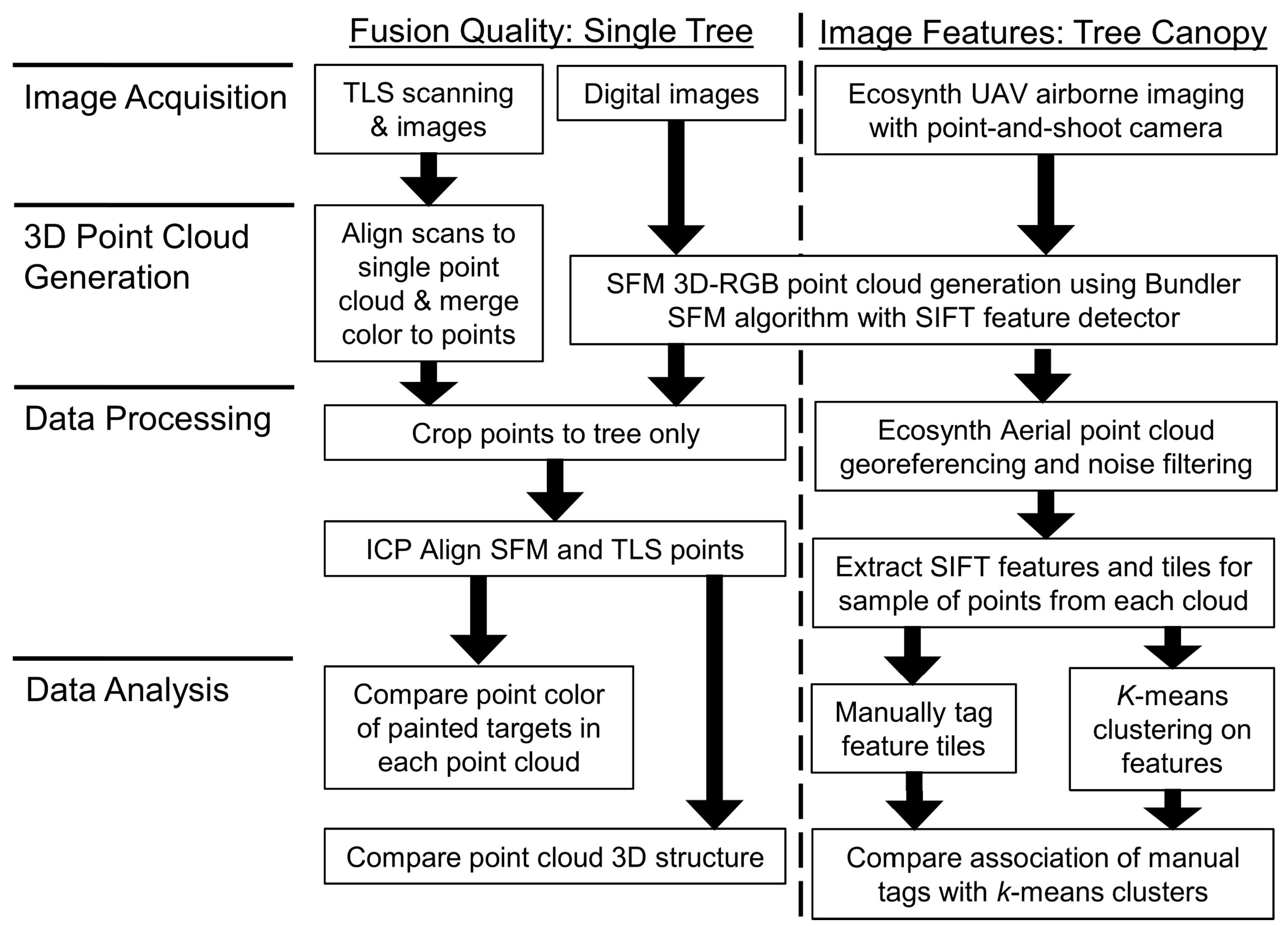
2. Materials and Methods

Data collection and analysis techniques are diagrammed in Figure 1 and are described below in two sections based on the main research objectives: evaluating the quality of SFM 3D-RGB fusion and assessing how vegetation is represented by SFM features.

2.1. Evaluating SFM 3D-RGB Fusion Quality

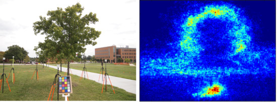
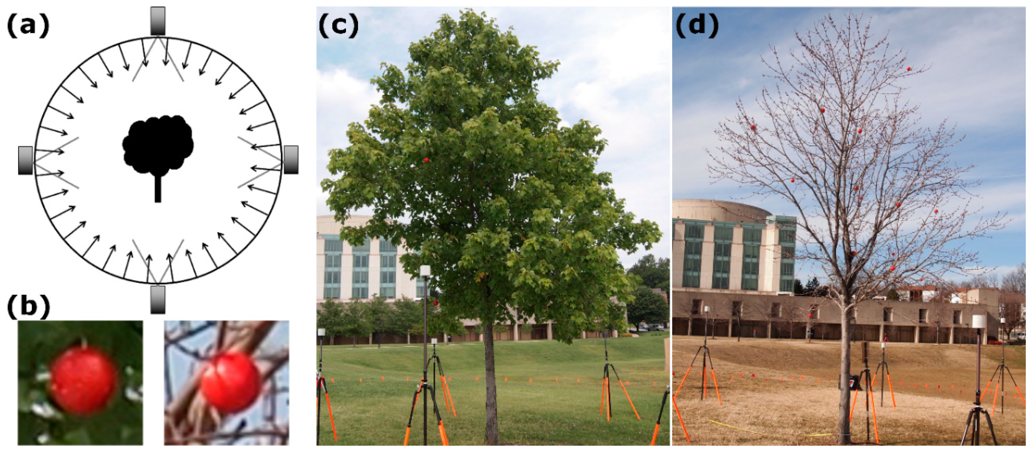
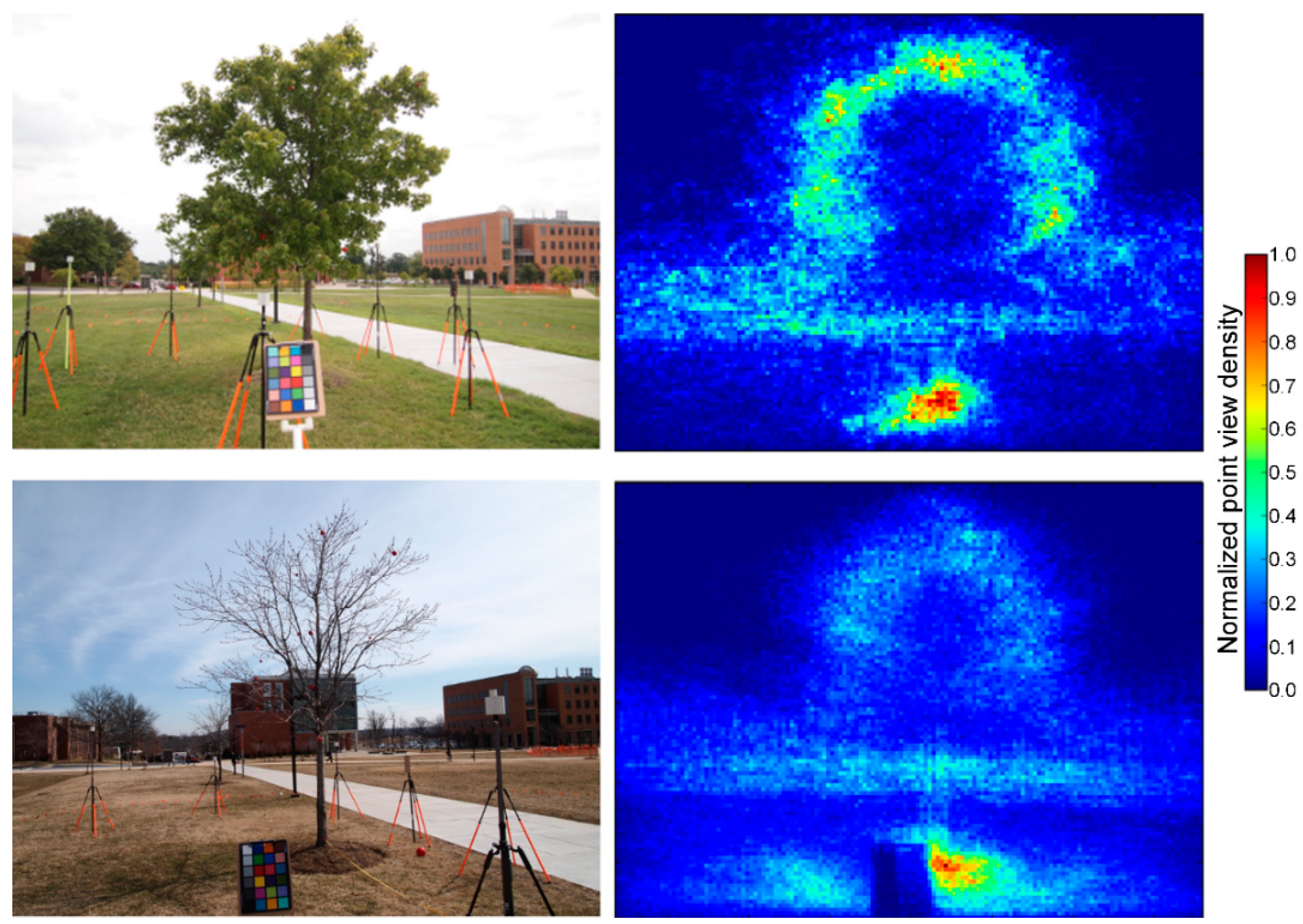
2.1.1. Ground-Based Scanning of a Single Tree

To evaluate the quality of SFM 3D-RGB fusion point clouds, a single free-standing tree was used to facilitate repeated imaging and to allow for the placement of painted targets to guide analysis. A red maple (Acer rubrum; height: 5.2 m; diameter at 1.37 m: 0.13 m) on the campus of the University of Maryland Baltimore County, Maryland, USA, was scanned under leaf-on (20 August 2012) and leaf-off (5 March 2013) conditions using an Olympus E-PL2 DSLR digital camera (14–42 mm lens) on a 2.0 m pole and a RIEGL VZ-400 terrestrial LIDAR scanner (TLS) equipped with a Nikon D700 DLSR digital camera with a (20 mm) lens for built-in LIDAR-color fusion. The TLS LIDAR height was 1.6 m and the accessory camera mount was located 0.4 m above this, or 2.0 m above the ground. Prior to scanning, foam balls (diameters: 0.05 m, 0.07 m, 0.15 m) were painted matte red and hung throughout the tree (leaf-on: n = 11; leaf-off: n = 14). In each season, SFM digital images and TLS scans were collected at the same time at roughly mid-day (10:00–14:00), to minimize the effect of shadows, but changes in lighting based on the relative location of the camera and sun were unavoidable. The lighting and weather varied from overcast to partly cloudy or clear on both days. With both camera systems, photos were taken with default ‘Auto’ shooting mode settings of focus, white balance, and shutter speed. Ten replicates of SFM digital images were taken at 2.5°/0.3 m intervals around the entire tree at a 7 m radius (≈144 images per replicate). Four TLS laser scans plus digital images were collected from orthogonal positions at a 7 m distance from the tree (i.e., north, east, south, and west). The single tree data collection configuration is diagrammed in Figure 2.

2.1.2. SFM 3D-RGB Point Clouds from Digital Images

3D-RGB point clouds were generated from ground image datasets using the open source Bundler SFM algorithm [26,38]. Bundler uses the Scale Invariant Feature Transform (SIFT) feature detector algorithm to identify features for matching across images [39]. The computation required an average of 12–24 h on a dual Intel Xeon X5670 workstation (12 compute cores) with 48GB of RAM running 64-bit Ubuntu 12.04. Single tree point cloud datasets were manually trimmed to only include the points of the tree. To compare the 3D structure derived from TLS and SFM point clouds, it was necessary to spatially align the point clouds in the same coordinate system [36]. All SFM and TLS point clouds were spatially co-registered by the iterative closest point (ICP) alignment method [40] within the open-source software Meshlab (v1.3.3 [41], described in Text S1). Point clouds were cropped to only include the tree (average points per point cloud: ≈80,000 leaf-on, ≈90,000 leaf-off).

2.1.3. TLS Data Processing

Leaf-on and leaf-off TLS scans were processed within the RISCAN-Pro software package (v1.7.3 release 6034) following the manufacturer’s instructions (detailed in Text S2). The reflective targets placed on tripods around the tree were used to automatically co-register individual TLS scans into a single 360° point cloud model. The same reflective targets were also used to manually refine the calibration between the TLS scans and digital images collected from the on-board DSLR, following the manufacturer’s instructions. The RGB color from the digital images was then automatically ‘fused’ to the 3D point cloud, based on the pixel color at the projection of each point into the corresponding image. The TLS point clouds were then manually trimmed to only include the points of the tree itself and exported into ASCII text files containing the XYZ location and RGB color of points. The trimmed TLS leaf-on point cloud contained 3,070,354 points and the leaf-off point cloud contained 926,215 points. To support the statistical comparison between TLS and SFM datasets, a set of 10 random samples was generated for each TLS point cloud as a form of pseudo-replication. The TLS replicates were sampled to produce new point clouds roughly matching the number and approximate average point count of the SFM point cloud replicates (≈90,000 points per replicate).

2.1.4. Extracting Points at Painted Targets

Threshold filtering based on the amplitude of the returned laser energy was used to identify the TLS points at painted targets [37]. The reflected laser energy at the targets was relatively higher than that of the surrounding foliage, but similar to large branches, so threshold-filtered point clouds were manually trimmed to remove any non-target points. For each target, a ‘target area’ was defined based on the TLS points associated with that target as a cube centered on the average of the XYZ coordinates with a side length equal to the average range in each XYZ dimension. Points in each TLS and SFM replicate falling inside the target areas were set aside for additional analysis.

2.1.5. Evaluation of 3D-RGB Fusion Quality

The accuracy of SFM fusion was evaluated by calculating the dominant hue color value of points observed in the target area relative to the red color of the painted targets, as defined by the range of hue color values (330°–20°) manually extracted from images of the targets [42,43]. A target was classified as ‘observed’ if the point cloud replicate contained one or more points within the target 3D search area. A ‘correct’ 3D-color fusion observation was one in which an average of >50% of the points observed at a target location had a hue color value within the red range.

2.2. Evaluation of Image Features from Tree Canopy Point Clouds

2.2.1. UAV Canopy Aerial Imagery

Aerial image data from prior research [3] collected using a point and shoot digital camera and a hobbyist multirotor UAV was used to evaluate the relationship between SFM image features, vegetation objects, and other types of landcover. Eight aerial image datasets represent three Temperate Deciduous forest areas in Maryland, USA, captured under varying conditions of flight altitude, levels of cloud cover (clear and overcast), wind, and the phenological state of the canopy (leaf-on, senescing, leaf-off), described in Table S3 and prior research.

2.2.2. SFM 3D-RGB Point Clouds from Digital Images

3D-RGB point clouds were generated from UAV imagery using the same Bundler SFM algorithm and workstation as described above (Section 2.1.2), requiring 27–552 h of computation. Aerial point cloud datasets of tree canopies were georeferenced to the WGS84 UTM Zone 18N projected coordinate system based on UAV GPS telemetry and were filtered using the Python-based free and open source Ecosynth online tools [44], following Dandois and Ellis [3].

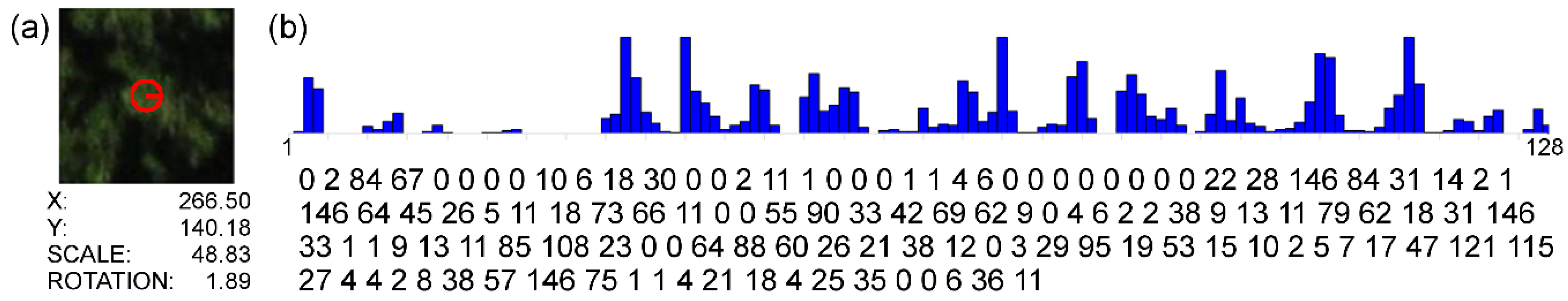
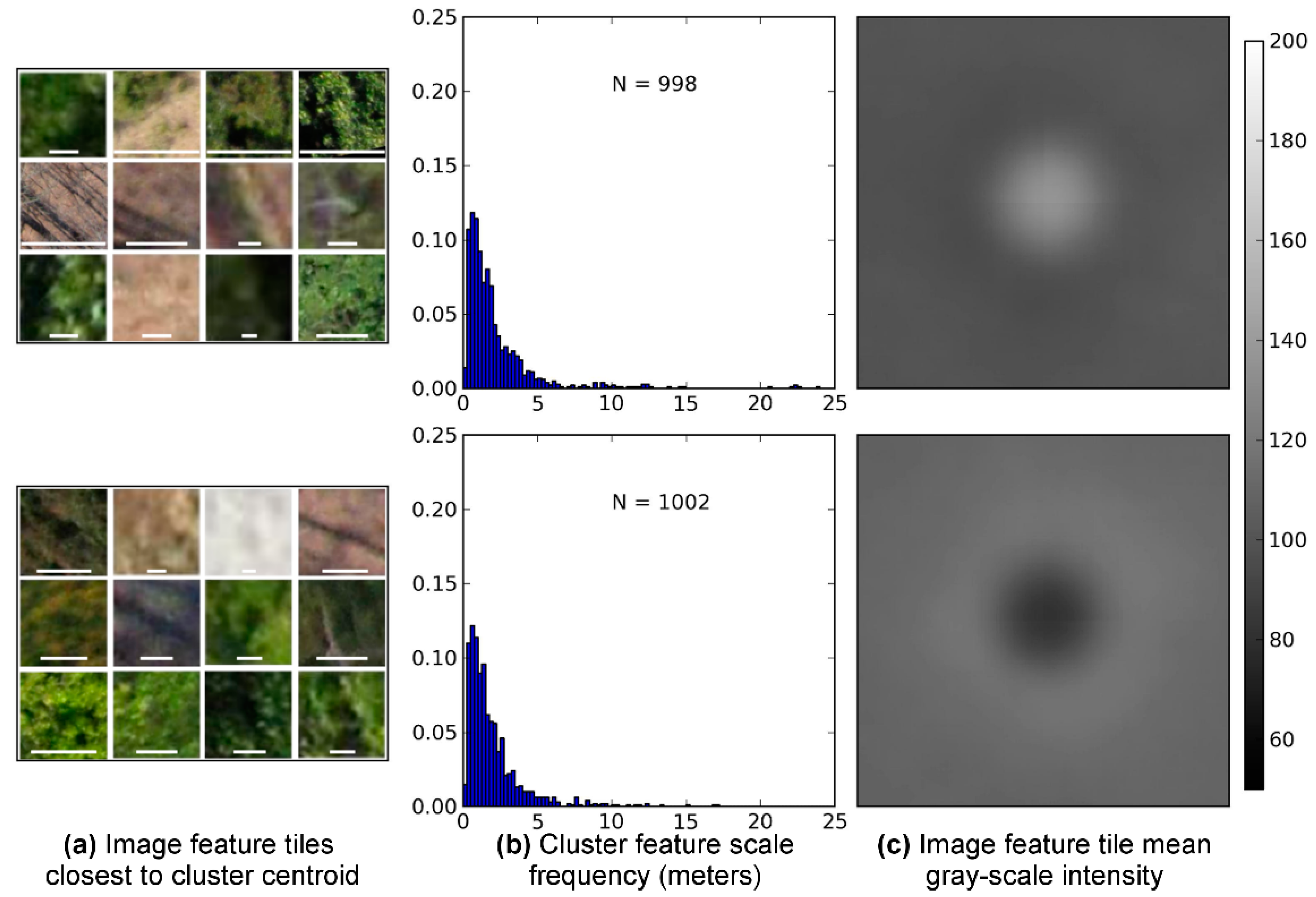
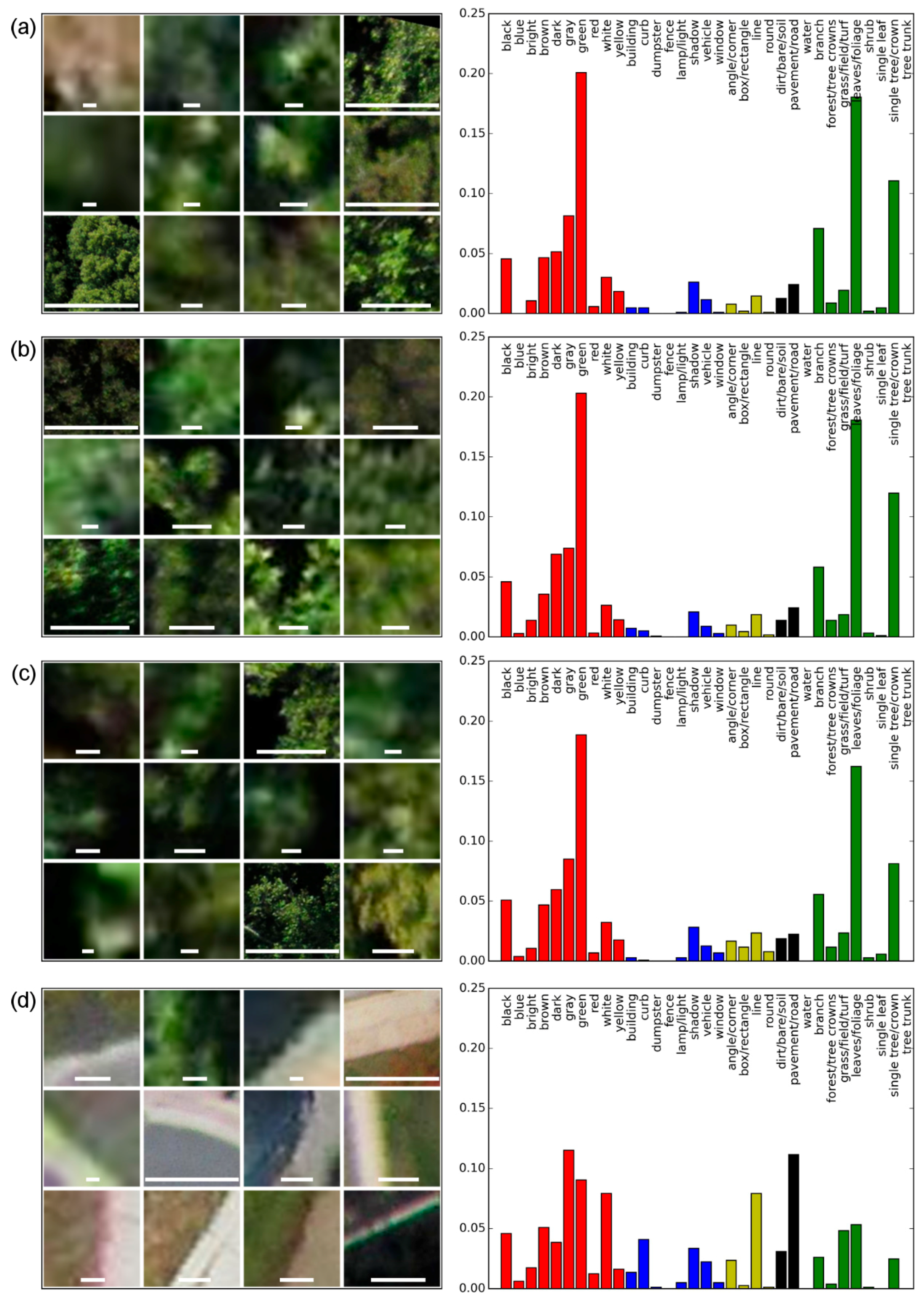
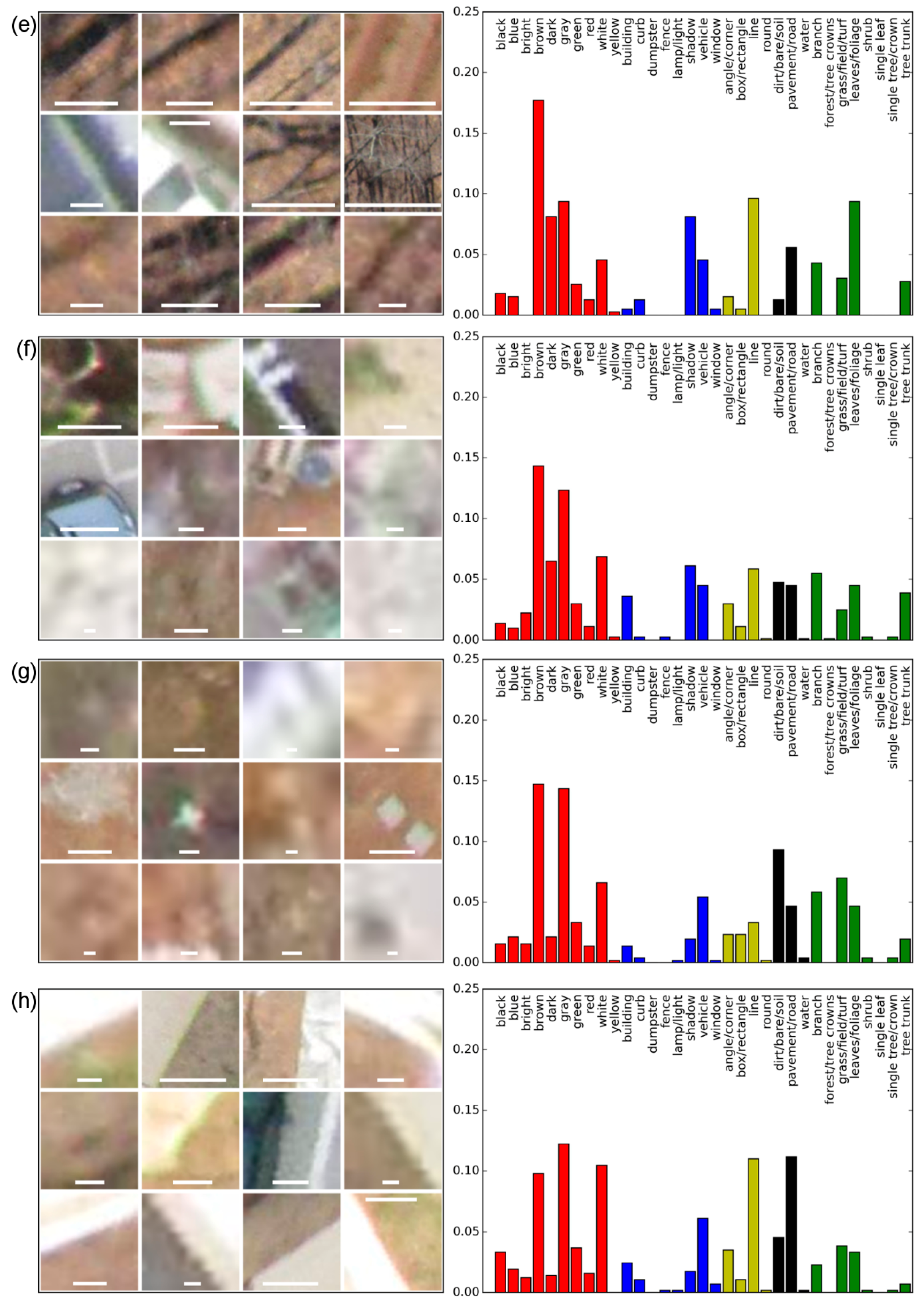
2.2.3. Extracting Image Features for SFM Point Clouds

The SIFT feature detector used in Bundler and other SFM algorithms, identifies feature points at the locations of local minima or maxima in the Difference of Gaussian (DOG) scale-space representation of a gray-scale version of the original image [39]. To do so, SIFT first produces a scale-space pyramid of the gray-scale image by iteratively Gaussian-blurring the image and then resampling it to a reduced resolution, simulating the effect of viewing the same scene from a greater distance. At each resampled resolution, the blurred image is subtracted from the previous one, to produce a stack of DOG images, highlighting distinct edges. A feature point is located at any pixel in a DOG image that is a maximum or minimum relative to the pixels immediately around it and the pixels above or below in the adjacent DOG pyramid stack. The reader is referred to Lowe [39] for a more detailed description of this process. Figure 3 provides an example of a single SIFT feature from an UAV image of a forest canopy. Figure 3a shows a small tile subset from an original larger image, with a red circle indicating where SIFT identified a ‘feature point’ in scale space. SIFT computes the X,Y location of that point in the original image, the scale of the feature (the radius of the red circle), and the orientation or rotation of the feature (the red line inside the circle). The SIFT feature descriptor is then computed across an area that is roughly 6× larger than the feature point (i.e., the entire image tile shown in Figure 3a) as the sum of the magnitude of gradients in eight primary directions within a 4 × 4 grid of sub-regions overlaid on the image feature tile [39], which, for visualization, can be displayed as a histogram, but is used by the algorithm as a 128 dimension (8 × 4 × 4 = 128D) numerical vector (Figure 3b).

To evaluate whether SFM points can be linked to discrete vegetation objects (e.g., leaves, branches, crowns, etc.), a collection of point ‘image features’ was extracted for a random sample of 250 points from each SFM aerial point cloud, producing a total of 2000 points. An image feature tile (Figure 3a) and 128D SIFT feature descriptor (Figure 3b) were extracted for each sampled point from the first Bundler image, following Li et al. [45].

2.2.4. Classification and Clustering of Image Features

To examine what SIFT features are being observed, an interactive graphical user interface (GUI) was developed in Python that allowed the user to see each image feature tile, view its relative location within an original image, and tag the feature with semantic tags (Figure S4). Users assigned descriptive tags from five categories (color, shape, surface, vegetation objects, and other objects) to each feature tile in the sample. K-means clustering was then carried out on the image feature 128D SIFT keys (Figure 3b) at multiple levels of k. Clustering stability analysis was used to determine the most stable number of clusters [43,46,47]. The frequency of manually identified tags for each cluster was then plotted to estimate the association of clusters to distinct semantic classes.

3. Results

3.1. Evaluation of SFM 3D-RGB Fusion Quality

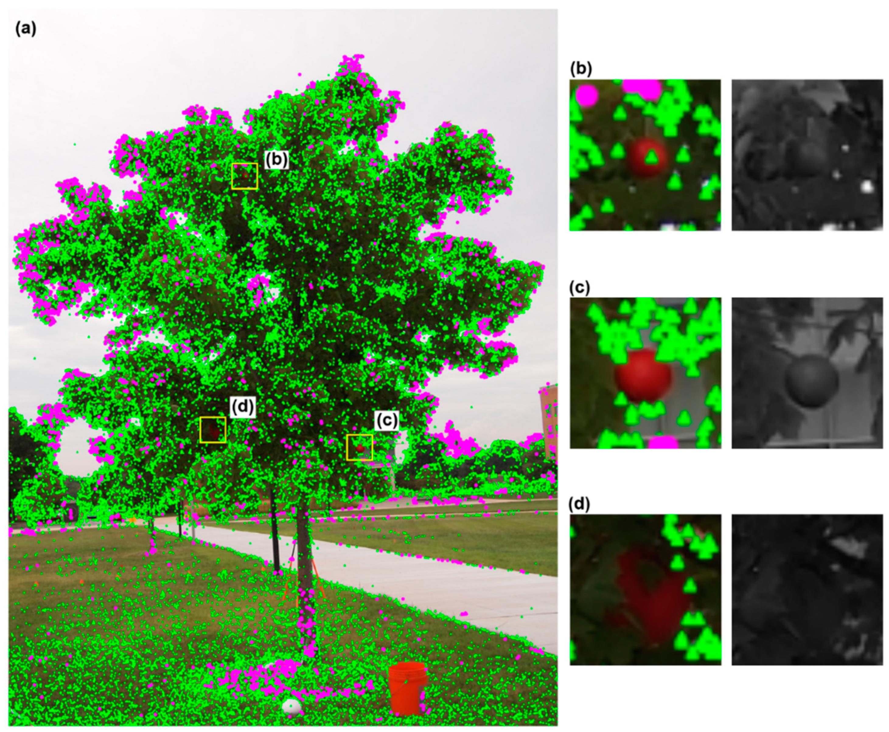
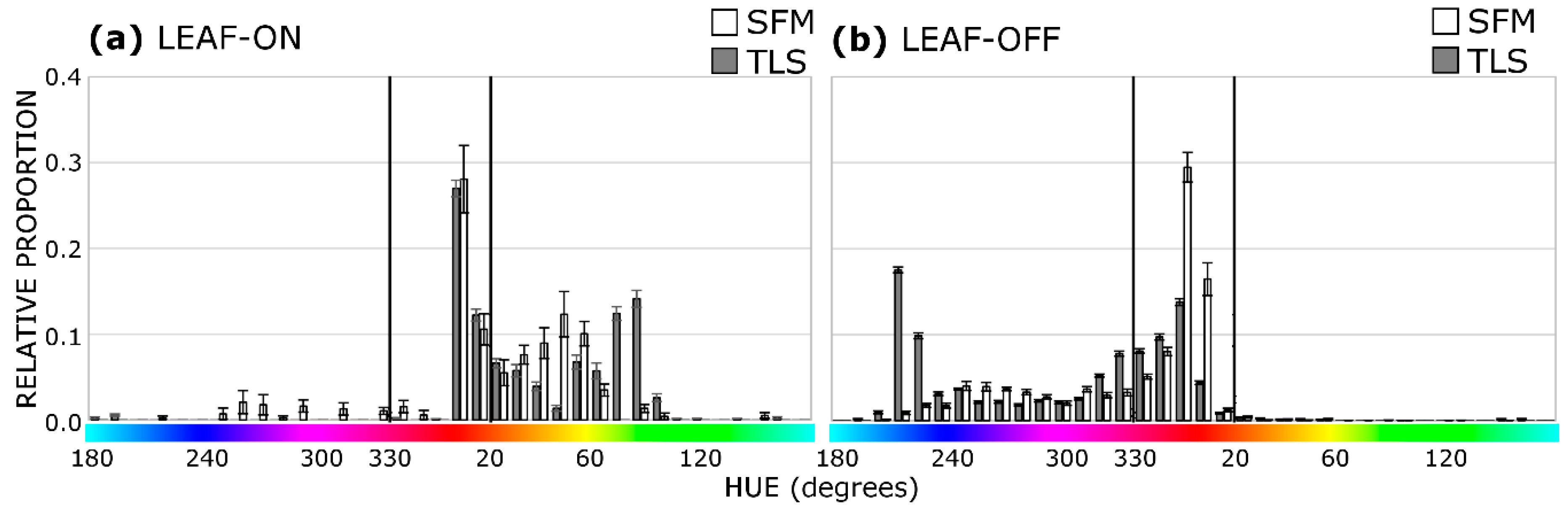
3.1.1. 3D-RGB Fusion Location and Color Accuracy

SFM and TLS fusion accuracy is reported in

Table 1. Target classification accuracy as error matrices between leaf-on and leaf-off TLS and SFM point clouds as the number of targets for which the average rate of observation of red points (red hue, 330°–20°) within the target 3D search area was greater than 50%.

(a)	TLS Leaf-on				(b)	TLS Leaf-off
		Red	Not red	Sum			Red	Not red	Sum
SFM Leaf-on	Red	1	2	3	SFM Leaf-off	Red	4	9	13
	Not red	4	4	8		Not red	0	1	1
	Sum	5	6	11		Sum	4	10	14
SFM Accuracy = 3/11 = 27%					SFM Accuracy = 13/14 = 93%
TLS Accuracy = 5/11 = 45%					TLS Accuracy = 4/14 = 29%
Overall Agreement = 5/11 = 45%					Overall Agreement = 5/14 = 36%
Kappa = −0.14					Kappa = 0.06

, in the form of classification error matrices for leaf-on and leaf-off ground-based point clouds of the tree test subject [25]. Classification accuracies differed by the fusion method and by the season based on the observation rates of the target points and the colors assigned to those points. SFM classification accuracy was the highest under leaf-off conditions (93%, Table 1b), where all targets were observed across all replicates. Under leaf-on conditions, SFM point clouds frequently observed no points or no red points at the targets, and as such , the classification accuracy was much lower (27%, Table 1a). TLS observed all targets under leaf-on and leaf-off conditions; however, these points were frequently not red, resulting in a higher classification accuracy than SFM in leaf-on conditions and a lower accuracy in leaf-off conditions (45% and 29%, respectively; Table 1). There was a weak agreement between the TLS and SFM classification of painted targets (45% and 36%), and the very small kappa values indicate that any agreement is probably due to chance alone, suggesting that the two systems observe the tree and targets differently.

Differences in the fusion classification accuracy due to the color assigned to the points can been be seen as peaks in the hue histogram (Figure 4), which provide an indication of the dominant colors [42]. These histograms highlight the average distribution of point hue inside the target areas for SFM and TLS point clouds under leaf-on and leaf-off conditions. Peaks inside the red hue region (330°–20°) represent points in the target area that had the correct color. For SFM, there is a distinct peak in the distribution of points in the red region under leaf-off conditions, with on average >60% of points having a red hue (Figure 4b), corresponding to a higher overall classification accuracy (Table 1b). Conversely, for SFM under leaf-on conditions, <40% of points had a red hue (Figure 4a), resulting in a lower classification accuracy (Table 1a).

Low observation rates of targets in the SFM leaf-on point clouds may be related to the behavior of the SIFT detector and feature matching. Figure 5 shows a single leaf-on image overlaid with all SIFT feature points identified in the image (green triangles) and those points that became part of the 3D point cloud (pink circles), representing approximately 7% of all points. The insets show examples of three painted red targets where no point cloud points were identified, even though the targets were visible in the RGB image. In some cases, SIFT identified a point at a fully visible target, but the point was not used in the point cloud for this view (Figure 5b), or points were only observed around the edges of the targets (Figure 5c). One target that was placed relatively deep inside the tree crown was not observed in any of the SFM replicates, that is, no SFM points were located at the location of the target, possibly due to shadowing or occlusion by leaves (e.g., Figure 5d). Targets that were not observed in SFM leaf-on point clouds were > 1 m from the outer hull of the tree, and there was a weak negative relationship between the average rate at which a target was observed and the distance to the outer hull of the tree (R² = 0.34, p-value < 0.1). Across all images in a replicate, 3D point cloud points tended to favor those SIFT features located around the outer edges of the tree crown, compared to the interior or bottom edge of the tree (Figure 6).

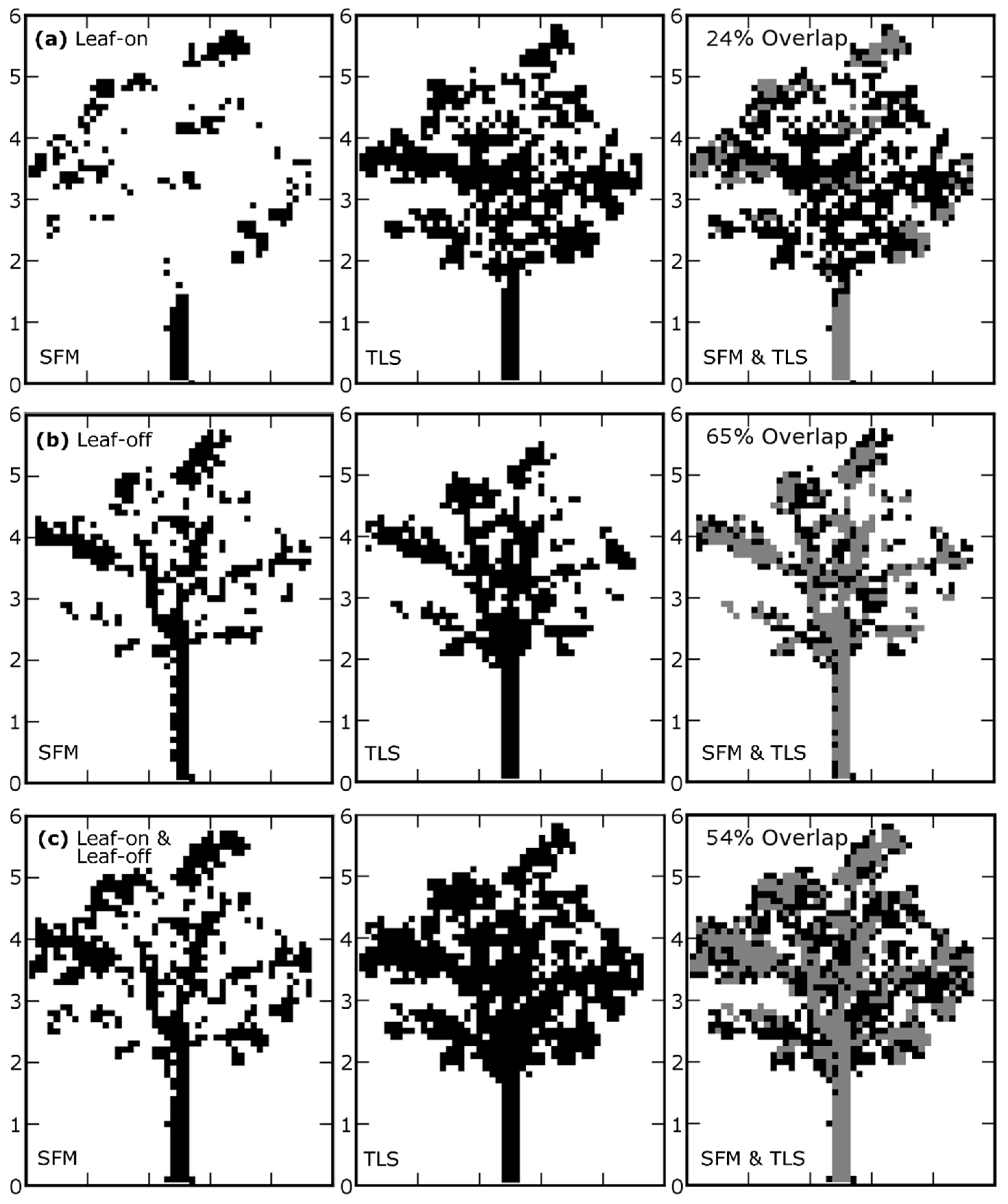
3.1.2. 3D Structure Quality

Similar to the results showing that SFM and TLS point clouds observed targets at different rates, there were also significant differences between the 3D structure of the tree, as observed by both systems. Vertical slices of 0.1 m voxel cubes (0.1 m × 0.1 m × 0.1 m = 0.001 m³) characterize where the tree structure (e.g., foliage, branches) was observed by each system, with at least one point per cube [48,49]. Leaf-on voxel slices of SFM point clouds primarily highlighted the exterior surface of the tree and had relatively few points in the interior of the tree compared to TLS (24% voxel overlap, Figure 7a). SFM leaf-off point clouds, however, revealed a much greater fraction of the tree interior and showed a greater similarity to those from TLS (65% overlap, Figure 7b). Comparing the voxel models of the merged leaf-on and leaf-off point clouds from SFM and TLS showed a higher overlap than leaf-on alone, but a lower overlap than leaf-off alone (54%, Figure 7c). Under leaf-on or leaf-off conditions, SFM observed the outer 3D structure of the tree just as well as the TLS scan replicates: there was no statistically significant difference in the relative vertical distribution of point cloud points along the length of the tree, either for leaf-on, leaf-off, or combined leaf-on and leaf-off point clouds (K-S test of distributions, p < 0.0001, Figure S5).

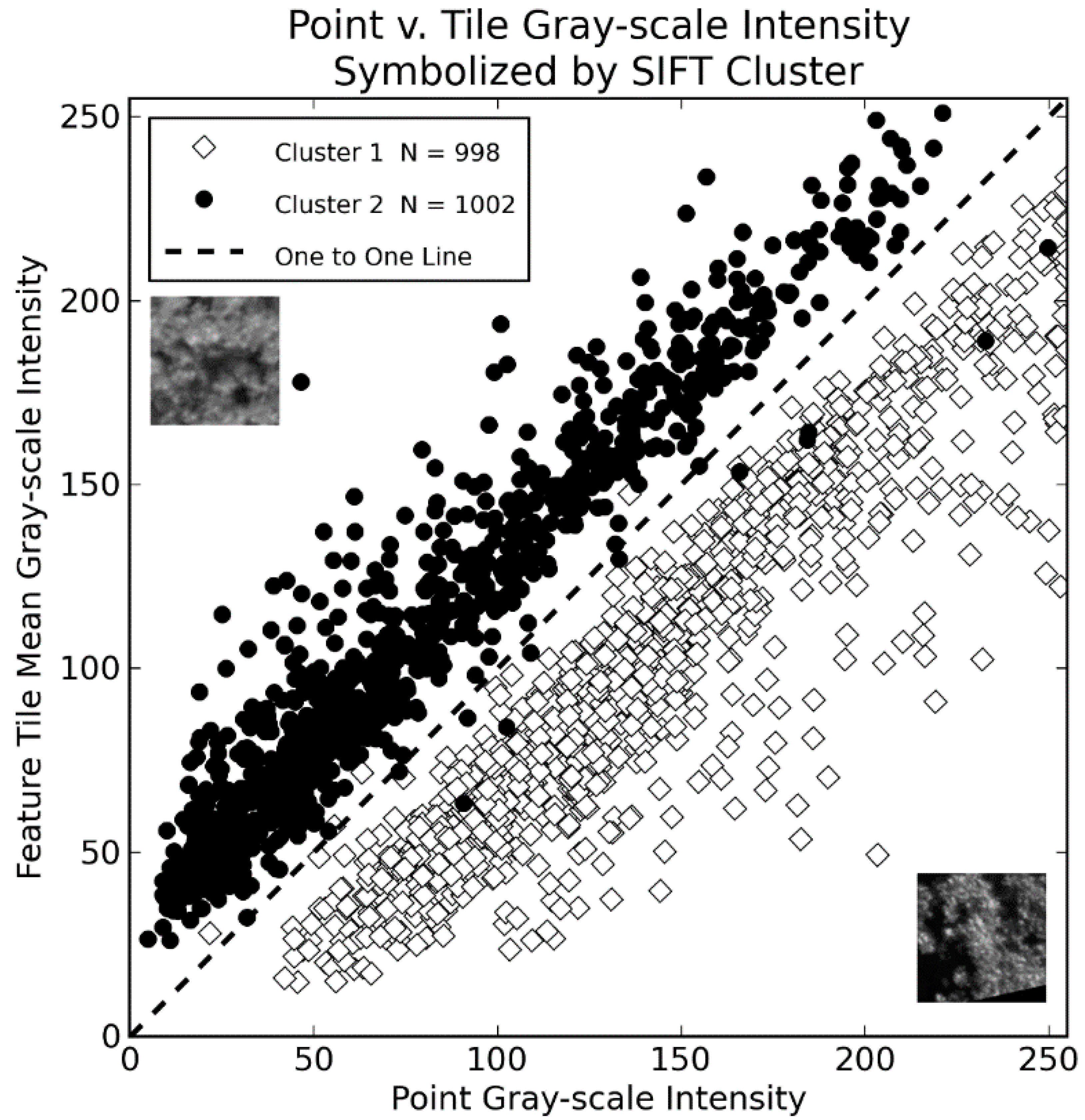
3.2. Evaluation of Image Features from Tree Canopy Point Clouds

K-means clustering of the 128D SIFT key descriptors from the SFM point cloud features consistently showed that image feature tiles cluster into two main groupings: points that are relatively brighter than the surroundings and points that are relatively darker than the immediate surroundings (Figure 8). The right panels in Figure 8c highlight this distinctive pattern by showing the average gray-scale intensity of all image feature tiles associated with a cluster, after the tiles had been resized to the same dimensions.

There was no significant difference between the metric scale of the image feature tiles associated with each cluster based on a Kruskal-Wallis non-parametric test of samples (Figure 8b). Similarly, a visual inspection of exemplar feature tiles, features closest to the cluster centroid, revealed no distinct patterns in the size of features per cluster (white bars in Figure 8a). These patterns were observed when clustering was performed on the entire set of 2000 features pooled from all datasets, for each individual set of 250 features sampled from each aerial dataset, and also for samples of 250 features from ground-based leaf-on and leaf-off point clouds of the single test tree (Figure S6). A comparison of the gray-scale intensity of the point color to the mean gray-scale intensity of the entire image feature tile around a point revealed the same pattern, with the sign of the difference between the point and the tile intensity being directly related to the cluster association for >99% of points (Figure 9).

Results of the manual identification (‘tagging’) of the image feature tiles are shown in Figure 10 for leaf-on and leaf-off datasets. In these figures, clusters are represented by exemplar feature tiles and as histograms showing the frequency of manually identified tags associated with each cluster. Leaf-on point clouds showed several clusters, with a high frequency of tags related to a forest landscape context that can be seen as the prominent histogram spikes for ‘green’, ‘leaves/foliage’, and ‘single tree/crown’ (Figure 10a–c). Clusters also described shapes and patterns, as can be seen for those that highlighted linear objects like tree shadows in leaf-off point clouds (Figure 10e) or the edges of sidewalks and pavements (Figure 10d,h), with corresponding peaks in tags of ‘line’ and ‘pavement/sidewalk’ that were not prominent in other clusters. Just as in the results shown in Figure 8 and Figure S6, clusters contained features at all scales, ranging from a few centimeters to >10 m, as can be seen in the exemplar tiles and white bars showing the original sizes of the tiles. While it was clear that clusters had some association with landscape context (e.g., forest vs. sidewalk and pavement), because they contained features at all scales, no cluster could be readily associated with distinct, scale-specific canopy object categories like leaves, branches, or crowns.

4. Discussion

The findings of this research are summarized in

Table 2. What is a point? Three primary traits of a SIFT-based SFM point cloud point.

	Image Sample	Numeric Feature Descriptor	3D Coordinate and RGB Color
Description	A portion of the original image, determined by the feature detector.	Numeric vector around a group of pixels, determined by the feature detector.	XYZ coordinates and RGB color with variable scale/size corresponding to part of the scene.
Quality	SIFT locates points that are brighter or darker than the surroundings.	Individually, a bright or dark spot, but not necessarily a distinct canopy object.	RGB color accurately describes object color if the object can be observed by the detector.
Implications	Sampling of a scene is determined by the feature detector.	Descriptors may be related to landscape context, but more information is needed to get to specific objects.	Fusion does not suffer occlusion effects as when different sensors are used, but will have omission errors due to feature detector.
Future Research	Examine how sampling of vegetation or parts of vegetation varies with different detectors.	Evaluate the use of multi-stage description of features including with color, scale, and other detectors.	Apply SFM 3D-RGB fusion to improve understanding of canopy color and structure, e.g., examining 3D dynamics of canopy phenology.

as a collection of the three primary traits of a SFM point cloud point: an image sample, a feature descriptor, and a 3D coordinate with RGB color. The quality of these traits—the accuracy of 3D location and color, whether something is observed or sampled, and how parts of the scene are characterized by the feature descriptors, is largely dependent upon the specific feature detector used for matching the points across images. Prior research has largely considered SFM point clouds based on their ‘LIDAR-like’ properties, primarily that structure is represented by a 3D point cloud. However, the work presented here suggests that understanding the quality of SFM point clouds is more complex than just quantifying the error of 3D measurements, and that a far richer dataset is available for as yet unexplored applications and areas of research.

4.1. Point as an Image Sample

The way in which a scene is sampled or observed by SFM is strongly dependent upon the behavior of the feature detector. SIFT placed points within the scene at places of high contrast that were either brighter or darker than the surroundings, which is to be expected given that the algorithm is designed to identify areas that are local minima or maxima within the scale-space pyramid [39]. This was observed when looking at feature clusters (Figure 10) and also when examining the spatial distribution of features and point cloud points with respect to the tree as a whole (Figure 5 and Figure 6). Parts of the image where no feature was produced, or which were unable to be successfully matched to the same feature in other images, were not ‘sampled’ in the point cloud, regardless of whether something was visible in an image. Similar observations were made in prior SFM research, where it was noted that no points were placed within areas of dark shadows [2,3], and that the density of point cloud points in the canopy could be influenced by image overlap and contrast [23]. Such situations are also present in other forms of remote sensing. For example, the spectral information of the land surface in satellite imagery is absent or significantly altered in areas that are heavily shadowed due to clouds [50]. With infrared LIDAR, no returns are recorded over areas of water because the laser pulse was absorbed instead of reflected back to the recording instrument [51]. Both LIDAR and optical imagery will sample space at different rates (pulse/pixel resolution), depending on the scale of observation and distance between the sensor and land surface, among many factors [17,24]. Given this, several options should be considered for improving scene sampling using SFM remote sensing, including using different feature descriptors, enhancing the image contrast, or using different image channels, and applying secondary processing techniques for creating denser point clouds [23].

4.2. Point as a Feature Descriptor

This study sought to use clustering and manually tagged features to identify groups of features specific to the forest canopy (e.g., leaf features, branch features, crown features, etc.). Prior research showed a strong relationship between SIFT image feature descriptors and different types of land cover observed in high resolution aerial images [35]. A comparison of the frequency with which manually identified tags occurred within clusters of SIFT features revealed similar patterns to prior research, in that clusters could be associated with different types of landcovers and different landscape contexts (e.g., forested vs. pavement; Figure 10). However, clusters contained features from all scales, from several cm to >10 m, which is to be expected given that the SIFT feature descriptor is designed to identify patterns invariant of scale, hence ‘Scale Invariant’ [39]. In comparison, the forest canopy structure is inherently organized into a spatial hierarchy that increases in spatial scale and complexity from the single leaf, up to groups of leaves, branches, crownlets, entire crowns, and the canopy as a whole [52]. For a feature detector to be used to identify distinct groups of features like a leaf or crown, spatial information is clearly needed as part of the classification process.

It is also important to consider that different types of detectors may be needed to identify features of canopy objects at different scales. For example, at the leaf scale, information about distinct lines, corners, and edges may be necessary for discriminating leaves from other canopy objects, and also for identifying leaves from different species [34]. At the crown scale, multi-scale, iterative, and region-based algorithms are applied to identify crown segments from individual high resolution imagery scenes [15], yet such algorithms are unlikely to be suitable for the 3D scene matching required for SFM. Color also plays an important role in discriminating amongst canopy objects, either manually or automatically, and was not considered here as part of the classification process. Other versions of SIFT make use of color information from images, such as hue, and may produce different and even better results for sampling the scene [53]. In addition, branch features tend to have gray or brown hues, while leaves typically have greenish hues, but may also have red, purple, yellow, orange, or brown hues, depending on the age and phenology of the leaf [3,12,33,54]. Advancing the ability to classify SFM point cloud points to distinct canopy objects using features will benefit from applying a multi-stage approach that makes use of other information including the scale, color, and shape extracted from images by several detectors. Indeed, this work only evaluated the canopy features in Temperate Deciduous forest canopies in Maryland, USA, and only under peak leaf-on and leaf-off phenological states. Evaluating SFM point cloud image features in different seasons or in different forests may reveal different feature typologies. Future research should evaluate forest canopy image features in different forests and under different phenological states, to attempt to identify objects like flowers, leaf buds, fruits, or even different overstory tree species.

4.3. Point as a 3D-RGB Point

The accuracy with which a 3D point cloud point was assigned the correct color strongly depended upon the way in which SIFT sampled the scene. When painted targets were clearly visible in photos and when SIFT placed features at targets that were then located in the 3D point cloud, those points had very high fusion accuracy, i.e., color was placed at the right location in the scene. Under these optimal conditions, SFM fusion was more accurate than that from the more advanced and expensive TLS and digital camera fusion measurements. This is likely due to the fact that the latter system requires the use of two sensors, each with a separate optical center, resulting in a spatial mismatch between the 3D and color information [20,21]. SFM point cloud points could be assigned a distinct metric scale, but the point scale varied by orders of magnitude (1 cm – >10 m), even within a single point cloud, owing to the fact that the SIFT feature detector was designed to identify ‘scale invariant’ features. This dramatically differs from the understanding of the fundamental units of LIDAR and optical imaging remote sensing, where the laser spot and pixel size are more consistent across an observation area. Future research should carefully consider how the varying scale of points is used when applying SFM point clouds to measure forest canopies. For example, the spatial scale of feature points, when combined with other feature descriptor information, may play a critical role in the classification of SFM 3D-RGB points to distinct canopy objects: e.g., leaves are likely the smallest features in the clusters where ‘green’, ‘leaves/foliage’ tags dominate.

One of the main objectives of this research was to determine whether SFM point clouds assign the correct color to a point in 3D space (Section 1.1). The results suggest that this is the case, especially under optimal conditions, where colored targets were clearly visible to the camera. However, since this work only examined the hue color value of targets, uncertainty remains about the true spectral or radiometric quality of SFM 3D-RGB point clouds. While measures like hue can in part remove some variations due to differences in illumination [55], multiple factors leading to variation in lighting were present in the study: varying lighting conditions (weather, cloud cover, angle between sun, camera and tree), differences in sensors, and sensor calibrations. Even so, it may be expected that given calibrated or normalized photos, similar results would be obtained in so far that SFM 3D color points would be placed in the correct location in 3D space. Future work should consider the radiometric quality of SFM 3D-RGB point clouds in the context of canopy features like flowers or leaves. For example, even tracking relatively coarse color descriptors like relative greenness can provide important insights into the phenology of forest canopies [54]. When analyzing the SFM point clouds of canopies obtained from UAV imaging, radiometrically calibrated color measures will also prove important for distinguishing among other canopy phenological states like deciduousness, fruiting, or flowering [56].

4.4. SFM and TLS See Vegetation Differently

Differences in the way in which SFM and TLS see vegetation were apparent when comparing the tomographic slices of 3D voxel models. SFM and TLS observed the outer 3D structure of the tree in a similar manner (Figure 7, Figure S4), and this result is in line with prior work that examined the relationship between the 3D structure of forest canopies observed by SFM from aerial images as compared to airborne LIDAR and field-based measurements [2,3,4]. The outer surface of the tree and forest canopy is a critical interface with the atmosphere, where important biophysical interactions with light, water, and air take place [52]. Even though SFM and TLS see vegetation differently, the results of this study strengthen those from prior research, that point to SFM as an accurate and effective substitute for LIDAR remote sensing of vegetation for certain applications and in certain contexts. For example, ground-based urban forest surveys are often interested in the height, shape, and volume of tree canopies for initializing ecosystem models [57,58]. Under such scenarios, SFM may be a viable and cheaper alternative for quickly observing the crown shape and volume. However, in other contexts where it is desirable to observe topography or suppressed vegetation under a dominant canopy, SFM will clearly experience difficulty in making such observations, and LIDAR would be the preferred remote sensing method. In addition, SFM can provide accurate 3D-RGB fusion, along with access to the rich field of computer vision image classification and recognition through the use of image features.

In this study, single TLS scans were sub-sampled to match the approximate point count of SFM point clouds to support statistical analysis, effectively reducing the high resolution of the TLS system to match that of the SFM data. While it may be expected that a single TLS point or pulse within a point cloud would have a predictable quality [24], it is unclear how the results of this study would vary if the TLS resolution was further increased or decreased, for example, by changing the sensor scan rates or by moving the instrument. Similarly, taking more photos or photos closer to the tree in SFM scans may also produce more or different feature points, resulting in different measurements of the canopy structure and color fusion. Indeed, prior research has shown that in the airborne, UAV context, SFM 3D-RGB models of vegetation have a varying quality, depending on the data collection conditions, including the resolution [23]. Future research comparing SFM and TLS or LIDAR observations of vegetation structure should also take into consideration the effective resolution of both systems.

5. Conclusions

This research has demonstrated that SFM algorithms can characterize vegetation structure with similar degrees of accuracy and better 3D-RGB fusion when compared to more advanced and expensive TLS systems. These results reinforce the growing body of literature pointing to SFM as a viable alternative to the accurate 3D-RGB remote sensing of the structural and spectral properties of vegetation at a high resolution and over small spatial extents. One of the key findings of this research was that the image feature detector algorithm, which is at the core of SFM 3D reconstruction, plays a critical role in defining the traits and quality of 3D-RGB point clouds. This research used an SFM algorithm based on the popular Scale Invariant Feature Transform (SIFT) feature detector. While some of the results of this work may be different if a different feature detector algorithm were used, the fact that the observation of tree and canopy vegetation by SFM is so strongly dependent upon the choice of the feature detector presents exciting new opportunities for computer vision ecology. Future work should consider the potential of hybrid approaches that combine SIFT with dedicated vegetation feature detectors based on the properties of plant, leaf, and flower color and structure [33,34]. By using a variety of computer vision feature detector algorithms (e.g., lines, edges, and corners for branches and leaves, regions and segments for crowns, color to distinguish among different feature types), within a decision-tree or other type of classifier, SFM remote sensing would move beyond simply recreating what is done with LIDAR. Such a fusion of 3D and spectral remote sensing with computer vision in a single sensor system would represent an exciting new frontier for remote sensing of the structural, spectral, and taxonomic complexity of forest ecosystems.

References

1. Anderson, K.; Gaston, K.J. Lightweight unmanned aerial vehicles will revolutionize spatial ecology. Front. Ecol. Environ. 2013, 11, 138–146. [Google Scholar] [CrossRef]
2. Dandois, J.P.; Ellis, E.C. Remote sensing of vegetation structure using computer vision. Remote Sens. 2010, 2, 1157–1176. [Google Scholar] [CrossRef]
3. Dandois, J.P.; Ellis, E.C. High spatial resolution three-dimensional mapping of vegetation spectral dynamics using computer vision. Remote Sens. Environ. 2013, 136, 259–276. [Google Scholar] [CrossRef]
4. Lisein, J.; Pierrot-Deseilligny, M.; Bonnet, S.; Lejeune, P. A photogrammetric workflow for the creation of a forest canopy height model from small unmanned aerial system imagery. Forests 2013, 4, 922–944. [Google Scholar] [CrossRef]
5. Zahawi, R.A.; Dandois, J.P.; Holl, K.D.; Nadwodny, D.; Reid, J.L.; Ellis, E.C. Using lightweight unmanned aerial vehicles to monitor tropical forest recovery. Biol. Conserv. 2015, 186, 287–295. [Google Scholar] [CrossRef]
6. Harwin, S.; Lucieer, A. Assessing the accuracy of georeferenced point clouds produced via multi-view stereopsis from unmanned aerial vehicle (UAV) imagery. Remote Sens. 2012, 4, 1573–1599. [Google Scholar] [CrossRef]
7. Javernick, L.; Brasington, J.; Caruso, B. Modeling the topography of shallow braided rivers using structure-from-motion photogrammetry. Geomorphology 2014, 213, 166–182. [Google Scholar] [CrossRef]
8. Westoby, M.J.; Brasington, J.; Glasser, N.F.; Hambrey, M.J.; Reynolds, J.M. ‘Structure-from-motion’ photogrammetry: A low-cost, effective tool for geoscience applications. Geomorphology 2012, 179, 300–314. [Google Scholar] [CrossRef]
9. Morgenroth, J.; Gomez, C. Assessment of tree structure using a 3D image analysis technique—A proof of concept. Urban For. Urban Green. 2014, 13, 198–203. [Google Scholar] [CrossRef]
10. Vitousek, P.; Asner, G.P.; Chadwick, O.A.; Hotchkiss, S. Landscape-level variation in forest structure and biogeochemistry across a substrate age gradient in hawaii. Ecology 2009, 90, 3074–3086. [Google Scholar] [CrossRef] [PubMed]
11. Erdody, T.L.; Moskal, L.M. Fusion of LIDAR and imagery for estimating forest canopy fuels. Remote Sens. Environ. 2010, 114, 725–737. [Google Scholar] [CrossRef]
12. Tooke, T.; Coops, N.; Goodwin, N.; Voogt, J. Extracting urban vegetation characteristics using spectral mixture analysis and decision tree classifications. Remote Sens. Environ. 2009, 113, 398–407. [Google Scholar] [CrossRef]
13. Asner, G.P.; Martin, R.E. Airborne spectranomics: Mapping canopy chemical and taxonomic diversity in tropical forests. Front. Ecol. Environ. 2009, 7, 269–276. [Google Scholar] [CrossRef]
14. Baldeck, C.A.; Asner, G.P.; Martin, R.E.; Anderson, C.B.; Knapp, D.E.; Kellner, J.R.; Wright, S.J. Operational tree species mapping in a diverse tropical forest with airborne imaging spectroscopy. PLoS ONE 2015, 10, e0118403. [Google Scholar] [CrossRef] [PubMed]
15. Ke, Y.; Quackenbush, L.J. A review of methods for automatic individual tree-crown detection and delineation from passive remote sensing. Int. J. Remote Sens. 2011, 32, 4725–4747. [Google Scholar] [CrossRef]
16. Geerling, G.; Labrador-Garcia, M.; Clevers, J.; Ragas, A.; Smits, A. Classification of floodplain vegetation by data fusion of spectral (CASI) and LIDAR data. Int. J. Remote Sens. 2007, 28, 4263–4284. [Google Scholar] [CrossRef]
17. Hudak, A.T.; Lefsky, M.A.; Cohen, W.B.; Berterretche, M. Integration of LIDAR and Landsat ETM+ data for estimating and mapping forest canopy height. Remote Sens. Environ. 2002, 82, 397–416. [Google Scholar] [CrossRef]
18. Mundt, J.T.; Streutker, D.R.; Glenn, N.F. Mapping sagebrush distribution using fusion of hyperspectral and LIDAR classifications. Photogramm. Eng. Remote Sens. 2006, 72, 47. [Google Scholar] [CrossRef]
19. Anderson, J.; Plourde, L.; Martin, M.; Braswell, B.; Smith, M.; Dubayah, R.; Hofton, M.; Blair, J. Integrating waveform LIDAR with hyperspectral imagery for inventory of a northern temperate forest. Remote Sens. Environ. 2008, 112, 1856–1870. [Google Scholar] [CrossRef]
20. Popescu, S.; Wynne, R. Seeing the trees in the forest: Using LIDAR and multispectral data fusion with local filtering and variable window size for estimating tree height. Photogramm. Eng. Remote Sens. 2004, 70, 589–604. [Google Scholar] [CrossRef]
21. Packalén, P.; Suvanto, A.; Maltamo, M. A two stage method to estimate speciesspecific growing stock. Photogramm. Eng. Remote Sens. 2009, 75, 1451–1460. [Google Scholar] [CrossRef]
22. Kampe, T.U.; Johnson, B.R.; Kuester, M.; Keller, M. Neon: The first continental-scale ecological observatory with airborne remote sensing of vegetation canopy biochemistry and structure. J. Appl. Remote Sens. 2010, 4, 043510. [Google Scholar] [CrossRef]
23. Dandois, J.P.; Olano, M.; Ellis, E.C. Optimal altitude, overlap, and weather conditions for computer vision uav estimates of forest structure. Remote Sens. 2015, 7, 13895–13920. [Google Scholar] [CrossRef]
24. Glennie, C. Rigorous 3D error analysis of kinematic scanning LIDAR systems. J. Appl. Geod. 2007, 1, 147–157. [Google Scholar] [CrossRef]
25. Congalton, R.G. A review of assessing the accuracy of classifications of remotely sensed data. Remote Sens. Environ. 1991, 37, 35–46. [Google Scholar] [CrossRef]
26. Snavely, N.; Seitz, S.; Szeliski, R. Photo Tourism: Exploring Photo Collections in 3D; The Association for Computing Machinery (ACM): New York, NY, USA, 2006; pp. 835–846. [Google Scholar]
27. Szeliski, R. Computer Vision; Springer: Berlin, Germany, 2011. [Google Scholar]
28. de Matías, J.; Sanjosé, J.J.D.; López-Nicolás, G.; Sagüés, C.; Guerrero, J.J. Photogrammetric methodology for the production of geomorphologic maps: Application to the veleta rock glacier (sierra nevada, granada, spain). Remote Sens. 2009, 1, 829–841. [Google Scholar] [CrossRef]
29. Huang, H.; Gong, P.; Cheng, X.; Clinton, N.; Li, Z. Improving measurement of forest structural parameters by co-registering of high resolution aerial imagery and low density LIDAR data. Sensors 2009, 9, 1541–1558. [Google Scholar] [CrossRef] [PubMed]
30. Lingua, A.; Marenchino, D.; Nex, F. Performance analysis of the sift operator for automatic feature extraction and matching in photogrammetric applications. Sensors 2009, 9, 3745–3766. [Google Scholar] [CrossRef] [PubMed]
31. Schwind, P.; Suri, S.; Reinartz, P.; Siebert, A. Applicability of the sift operator to geometric SAR image registration. Int. J. Remote Sens. 2010, 31, 1959–1980. [Google Scholar] [CrossRef]
32. Beijborn, O.; Edmunds, P.J.; Kline, D.I.; Mitchell, B.G.; Kriegman, D. Automated annotation of coral reef survey images. In Proceedings of the 2012 IEEE Conference on Computer Vision and Pattern Recognition, Providence, RI, USA, 16–21 June 2012; pp. 1170–1177. [Google Scholar]
33. Kendal, D.; Hauser, C.E.; Garrard, G.E.; Jellinek, S.; Giljohann, K.M.; Moore, J.L. Quantifying plant colour and colour difference as perceived by humans using digital images. PLoS ONE 2013, 8, e72296. [Google Scholar] [CrossRef] [PubMed]
34. Nilsback, M.-E. An Automatic Visual Flora—Segmentation and Classication of Flower Images; University of Oxford: Oxford, UK, 2009. [Google Scholar]
35. Yang, Y.; Newsam, S. Geographic image retrieval using local invariant features. IEEE Trans. Geosci. Remote Sens. 2013, 51, 818–832. [Google Scholar] [CrossRef]
36. Hosoi, F.; Nakai, Y.; Omasa, K. Estimation and error analysis of woody canopy leaf area density profiles using 3-d airborne and ground-based scanning LIDAR remote-sensing techniques. IEEE Trans. Geosci. Remote Sens. 2010, 48, 2215–2223. [Google Scholar] [CrossRef]
37. Seielstad, C.; Stonesifer, C.; Rowell, E.; Queen, L. Deriving fuel mass by size class in douglas-fir (pseudotsuga menziesii) using terrestrial laser scanning. Remote Sens. 2011, 3, 1691–1709. [Google Scholar] [CrossRef]
38. Bundler v0.4. Available online: https://www.cs.cornell.edu/~snavely/bundler/ (accessed on 11 February 2017).
39. Lowe, D.G. Distinctive image features from scale-invariant keypoints. Int. J. Comput. Vis. 2004, 60, 91–110. [Google Scholar] [CrossRef]
40. Besl, P.J.; McKay, H.D. A method for registration of 3-d shapes. IEEE Trans. Pattern Anal. Mach. Intell. 1992, 14, 239–256. [Google Scholar] [CrossRef]
41. Meshlab v1.3.3 64-bit. Available online: http://www.meshlab.net/ (accessed on 11 February 2017).
42. Aptoula, E.; Lefèvre, S. Morphological description of color images for content-based image retrieval. IEEE Trans. Image Process. 2009, 18, 2505–2517. [Google Scholar] [CrossRef] [PubMed]
43. Manjunath, B.S.; Ohm, J.R.; Vasudevan, V.V.; Yamada, A. Color and texture descriptors. IEEE Trans. Circuits Syst. Video Technol. 2001, 11, 703–715. [Google Scholar] [CrossRef]
44. Ecosynth Aerial v1.0. Available online: http://code.ecosynth.org/EcosynthAerial (accessed on 11 February 2017).
45. Li, Y.; Snavely, N.; Huttenlocher, D. Location recognition using prioritized feature matching. In Computer Vision ECCV 2010 Lecture Notes in Computer Science; Springer: Berlin, Germany, 2011; pp. 791–804. [Google Scholar]
46. Jain, A.K. Data clustering: 50 years beyond k-means. Pattern Recognit. Lett. 2010, 31, 651–666. [Google Scholar] [CrossRef]
47. Lange, T.; Roth, V.; Braun, M.L.; Buhmann, J.M. Stability-based validation of clustering solutions. Neural Comput. 2004, 16, 1299–1323. [Google Scholar] [CrossRef] [PubMed]
48. Holden, M.; Hill, D.L.G.; Denton, E.R.E.; Jarosz, J.M.; Cox, T.C.S.; Rohlfing, T.; Goodey, J.; Hawkes, D.J. Voxel similarity measures for 3-d serial mr brain image registration. IEEE Trans. Med. Imaging 2000, 19, 94–102. [Google Scholar] [CrossRef] [PubMed]
49. Parker, G.; Harding, D.; Berger, M. A portable LIDAR system for rapid determination of forest canopy structure. J. Appl. Ecol. 2004, 41, 755–767. [Google Scholar] [CrossRef]
50. Huang, C.; Thomas, N.; Goward, S.N.; Masek, J.G.; Zhu, Z.; Townshend, J.R.G.; Vogelmann, J.E. Automated masking of cloud and cloud shadow for forest change analysis using Landsat images. Int. J. Remote Sens. 2010, 31, 5449–5464. [Google Scholar] [CrossRef]
51. McKean, J.; Isaak, D.; Wright, W. Improving stream studies with a small-footprint green LIDAR. Eos Trans. Am. Geophys. Union 2009, 90, 341–342. [Google Scholar] [CrossRef]
52. Parker, G.G. Structure and microclimate of forest canopies. In Forest Canopies: A review of Research on a Biological Frontier; Lowman, M., Nadkarni, N., Eds.; Academic Press: San Diego, CA, USA, 1995; pp. 73–106. [Google Scholar]
53. Van de Sande, K.E.A.; Gevers, T.; Snoek, C.G.M. Evaluating color descriptors for object and scene recognition. IEEE Trans. Pattern Anal. Mach. Intell. 2010, 32, 1582–1596. [Google Scholar] [CrossRef] [PubMed]
54. Keenan, T.F.; Darby, B.; Felts, E.; Sonnentag, O.; Friedl, M.A.; Hufkens, K.; O’Keefe, J.; Klosterman, S.; Munger, J.W.; Toomey, M.; et al. Tracking forest phenology and seasonal physiology using digital repeat photography: A critical assessment. Ecol. Appl. 2014, 24, 1478–1489. [Google Scholar] [CrossRef]
55. Mizunuma, T.; Wilkinson, M.; Eaton, E.L.; Mencuccini, M.; Morison, J.I.L.; Grace, J. The relationship between carbon dioxide uptake and canopy colour from two camera systems in a deciduous forest in southern England. Funct. Ecol. 2013, 27, 196–207. [Google Scholar] [CrossRef]
56. Garzon-Lopez, C.X.; Bohlman, S.A.; Olff, H.; Jansen, P.A. Mapping tropical forest trees using high-resolution aerial digital photographs. Biotropica 2013, 45, 308–316. [Google Scholar] [CrossRef]
57. Lefsky, M.; McHale, M.R. Volume estimates of trees with complex architecture from terrestrial laser scanning. J. Appl. Remote Sens. 2008, 2, 023521. [Google Scholar]
58. McHale, M.R.; Burke, I.C.; Lefsky, M.A.; Peper, P.J.; McPherson, E.G. Urban forest biomass estimates: Is it important to use allometric relationships developed specifically for urban trees? Urban Ecosyst. 2009, 12, 95–113. [Google Scholar] [CrossRef]
Figure 1. Workflow diagram describing the data collection, processing, and analysis used for evaluating SFM 3D-RGB point cloud fusion quality and image feature characteristics. Acronyms: TLS, terrestrial laser scanner; UAV, unmanned aerial vehicle; SFM, structure from motion; SIFT, scale invariant feature transform; ICP, iterative closest point. Ecosynth refers to techniques described in [2,3].
Remotesensing 09 00355 g001
Figure 2. Single tree data collection configuration with TLS locations indicated by gray boxes and SFM image locations represented by arrows (a), painted red foam balls in the tree under leaf-on and leaf-off conditions (b), view of the tree with painted targets from approximately the same point of view under leaf-on (c) and leaf-off (d) conditions.
Remotesensing 09 00355 g002
Figure 3. A single ‘image feature tile’ with a circle indicating the scale of the SIFT feature (a), and the 128-D SIFT image feature descriptor as a histogram and numerical vector (b).
Remotesensing 09 00355 g003
Figure 4. Mean histograms of point hue for points that fell inside the target areas for SFM (white bars) and TLS (gray bars) point clouds under leaf-on and leaf-off conditions. Error bars are standard error (n = 10). Black vertical lines are red hue cutoff region (330°–20°).
Remotesensing 09 00355 g004
Figure 5. Example of the role of the SIFT detector in the placement of point cloud points. (a) original image overlaid with all SIFT points (green triangles) and point cloud points (pink circles), (bd) insets show targets that were not assigned a point cloud point for this view, with the associated gray-scale version of each inset at right.
Remotesensing 09 00355 g005
Figure 6. Left panels: example images used in single tree SFM reconstruction under leaf on (top) and leaf off (bottom) conditions. Right panels: view density plots showing the density of where point cloud points were viewed within each image for all images and views from a single replicate. Density is aggregated to 25 × 25 pixel bins, normalized to the total number of points per cloud, and rescaled from 0–1 for comparison. Point views counted in these plots correspond to the pink circles in Figure 5.
Remotesensing 09 00355 g006
Figure 7. Tomographic slices of a 0.1 m section of leaf-on (a), leaf-off (b), combined leaf-on and leaf-off (c) SFM and TLS point clouds. Pixels represent a 0.1 m × 0.1 m × 0.1 m cube within which at least 1 point was located. All slices are co-registered to the same coordinate system and viewpoint. Right panels indicate the degree of voxel overlap between SFM and TLS in gray.
Remotesensing 09 00355 g007
Figure 8. Clustering results (k = 2) on SIFT 128D descriptors for 2000 points from aerial SFM point clouds. Left panels (a) show 12 image feature tiles closest to cluster centroid with white bars indicating the original feature tile scale. Center panels (b) show the frequency distribution of the scale (meters) of cluster features. Right panels (c) show the ‘mean gray-scale intensity’ of all cluster image feature tiles resized to the same size (200 pixels square).
Remotesensing 09 00355 g008
Figure 9. Scatter plot of the gray-scale intensity of points versus the mean gray-scale intensity of the image feature tile around each point, symbolized by the same SIFT clusters as in Figure 7. Points located below the one-to-one line have a point that is brighter than its surroundings, points above the line are darker than the surroundings, as shown in the example images.
Remotesensing 09 00355 g009
Figure 10. (ah) Exemplar cluster feature tiles (left) and frequency distributions (right) of tags per image feature cluster for leaf-on aerial point clouds. Tiles are those closest to cluster centroid. White bars indicate original tile size. Bar color represents tag category: red = colors, blue = objects, yellow = shapes, black = other surfaces, green = vegetation.
Remotesensing 09 00355 g010aRemotesensing 09 00355 g010b