Temperature Compensation for Radiometric Correction of Terrestrial LiDAR Intensity Data

Abstract

Correction of terrestrial Light Detection and Ranging (LiDAR) intensity data has been increasingly studied in recent years. The purpose is to obtain additional insight into the scanned environment that is not available from the geometric information alone. Radiometric correction, as the name implies, corrects the received intensity to standard reflectance values in the range of $(0,1)$. This correction typically compensates for the dependence of angle and distance. This paper presents an additional compensation for temperature that may be necessary for some LiDAR instruments such as the Faro Focus${}^{3\mathrm{D}}$ X 330 laser scanner. It is also shown that temperature compensation is not necessary for the Riegl VZ–400. Another important contribution of this work is the verification of a previously published radiometric correction in different environments. The correction was applied to two different Terrestrial Laser Scanner (TLS) instruments: a Faro Focus${}^{3\mathrm{D}}$ X 330 and Riegl VZ-400. Overall, the VZ-400, without temperature compensation, produced better results with a Root Mean Square (RMS) of the standard deviation of error being 0.053 and a RMS of the mean error of 0.036 compared to 0.069 and 0.046 for the Faro Focus${}^{3\mathrm{D}}$ X 330. It was found, for the case of the Faro device, that the temperature of the instrument played an important role in the accuracy of the results. The proposed temperature compensation method improved the RMS standard deviation of the error by 1.4 times and the RMS of the error by 2.6 times, compared to the uncompensated results.

1. Introduction

Terrestrial Light Detection and Ranging (LiDAR) intensity data correction has been increasingly studied in recent years to obtain additional insight into the scanned environments that is not available from the geometric information alone. This additional intensity information has the possibility of aiding automated processing techniques [1,2,3,4,5,6,7]. In essence, it provides a value that has some dependence on the material properties of the surface, which reflected the laser light. The raw intensity data provided by Terrestrial Laser Scanners (TLSs) is a Digital Number (DN) that is assumed to be proportional to the received power. However, each different scanner and scanner manufacturer reports intensity differently so direct comparisons of intensity values between manufacturers and devices are not trivial. The aim of radiometric correction, in our case, is to provide a number between zero and one, calibrated to known diffuse reflectance standards. The advantages of having a consistent corrected value is that it can be compared across scanners and across different environments. This allows manual and automatic algorithms to be developed that can be seamlessly applied across different instruments and manufacturers.

It is commonly accepted that the intensity value is dependent upon four factors: instrument and environmental factors, surface properties of the target and measurement geometry [8]. In most previous work, correcting for measurement geometry was the main focus. This mainly involved applying a distance correction [9,10], an angle correction [11,12] or both an angle and distance correction [8,13,14,15,16,17,18,19,20]. Some of the previous work has assumed a diffuse surface so that the corrected intensity becomes the diffuse reflectance [13,14,18] or pseudoreflectance [17]. However, since many materials, especially manmade materials, produce specular reflections or have varying surface roughness, more complex reflectance models have been used [8,11,15,19,20]. There are two main drawbacks to using a more complex reflectance model: (1) the model requires an additional parameter related to the roughness of the surface being scanned; and (2) the estimated values can no longer be easily calibrated completely with a diffuse reflectance target. This second reason is very important when verifying the model. Without calibrating the model to a known standard, it is difficult to appropriately verify the model in different environments and conditions. Much of the literature has failed to do verification on their models and, in fact, their reported results are often the modelling errors and not the actual errors one would expect to see on a new data set [13,14,17]. In addition, many studies do not correct to a known diffuse reflectance standard value and instead use a normalized, or corrected intensity [9,15,19].

The genesis of this research came out of verifying the model presented in [18]. During verification of the model for the Faro Focus${}^{3\mathrm{D}}$ X 330 (Lake Mary, FL, USA) [21], it was discovered that the model performed very poorly on new data sets. A number of possible causes for the poor performance were investigated. This work led to the ambient temperature being the problem. A temperature calibration method for the Faro Focus ${}^{3\mathrm{D}}$ X 330 laser scanner was developed and is presented in this paper. It is also shown how such a temperature compensation is not necessary for the Riegl VZ-400 (Horn, Austria) [22] through three verification experiments. In both cases, the radiometric calibration method is based on the work by Errington et al. [18]. To the best of the authors’ knowledge, this is the first time that a temperature compensation has been applied to intensity correction for terrestrial laser scanners. Another important contribution of this work is the verification of the radiometric correction and temperature compensation in different environments.

The following section highlights some of the most relevant and recent work in the area of intensity correction and Section 3 presents the reflectance estimation model used in this research. The temperature compensation method is presented in Section 4 and the experiments showing its applicability are described in Section 5. Results and Discussions are presented in Section 6 and Section 7, respectively, and finally, in Section 8, conclusions and a summary are presented.

2. Related Work

This section provides a brief overview of the most recent and relevant literature related to terrestrial LiDAR intensity correction. Fang et al. [15] proposed an angle and distance correction for the Z+F Imager5006i (Wangen im Allgäu, Germany), which estimates parameters of a customized laser transmission function for the specific scanner. They performed the calibration of the model with paper targets at angles between 0 and 80 degrees and distances between 0 and 50 m. Similar to previous research, they focused on minimizing the variation of corrected intensities and not calibrating their model to known reflectances.

Tan and Cheng [17] modelled the received intensity as a multiplicative function of three polynomials of reflectance $\rho$, cosine of the angle, $cos\theta$, and distance, R. In their case, they calibrated this model with diffuse reflectance targets (20%, 40%, 60% and 80%) for the Faro Focus${}^{3\mathrm{D}}$ X 330 and Faro Focus${}^{3\mathrm{D}}$ 120. The only verification of their model was done by comparing the variability of the corrected intensity using real world data. Similarily, in Tan et al. [9], they investigate just a distance correction, through a polynomial series, and apply the model to the two Faro scanners, as in [17].

Zhu et al. use intensity measured by a Riegl VZ-400 to estimate plant leaf water content [11]. Their correction is not generally applicable because it was performed at a single distance. However, they did propose modelling the received intensity as a combination of diffuse and specular components. This was necessary due to the highly specular nature of many of the leaf species being scanned.

Carrea et al. [19] proposed using the Oren–Nayar reflectance model [23], which incorporates a more realistic model of diffuse surfaces than the typical Lambertian model, in order to correct for both distance and angle. They apply their correction to lithological differentiation. A drawback of their approach, and other reflectance models that take into account surface roughness, is the additional parameters required for the surface types scanned.

Tan et al. [20] also propose a method using the Oren–Nayar reflectance model. They apply their method to the Faro Focus${}^{3\mathrm{D}}$.

3. Model Description and Fitting Approach

The method used here to correct the returned intensity was first presented in [18]. It was inspired by the work of Pfeifer et al. [14]. Although this method is not central to the contributions in this paper, it is presented for completeness.

In general, it is desired to model the returned intensity, I, as a function of the angle of incidence, $\alpha$, the reflectance of the surface, $\rho$, and the distance from the scanner to the point of interest, r. Mathematically this dependence is,

$$I=g(k;\mathbf{P}(r\left)\right),$$

(1)

where $k=\rho cos\alpha$ and $\mathbf{P}$ is a set of parameters that depend upon r. The specific model used here that provides excellent performance and yet is relatively straight forward is

$$I=p_1\left(r\right)ln\left(k\right)+p_2\left(r\right),$$

(2)

where the dependence of the parameters $p_1$ and $p_2$ on the distance r has been made explicit. This model was determined empirically from a number of different forms. The natural logarithm dependence performed the best out of all the other model forms tested. Equation (2) can then be solved for the reflectance $\rho$, which yields

$$\widehat{\rho }=\frac{1}{cos\alpha }exp\left({\displaystyle \frac{I-p_2\left(r\right)}{p_1\left(r\right)}}\right),$$

(3)

where the hat above the $\rho$ implies that it is an estimate of the true reflectance, $\rho$.

To calibrate this model for a specific laser scanner, it is necessary to collect data points ${\mathbf{d}}_i={[{\alpha }_i,r_i,I_i]}^T$, with corresponding known reflectance ${\rho }_i$, where T represents the transpose and the ith data point is composed of an incidence angle ${\alpha }_i$, distance $r_i$, and a returned intensity $I_i$. A typical objective function to be minimized is the squared residuals between the true and estimated reflectance which has the following form,

$$J\left(\mathbf{P}\right)=\sum _{i=1}^N{[{\widehat{\rho }}_i({\mathbf{d}}_i;\mathbf{P})-{\rho }_i]}^2,$$

(4)

where it is assumed that there are N data points. For the form of the model presented here, this approach is not practical, since the parameters $p_1\left(r\right)$ and $p_2\left(r\right)$ are a function of distance. Instead, the experiments are designed so that multiple incidence angles are collected at each distance. In this way, each distance r is held fixed while the parameters, which minimize Equation (4), are found.

Once the optimization at each value of r has been completed, it results in a matrix $\mathbf{P}$ that provides $p_1$ and $p_2$ at different values of r:

$$\mathbf{P}=\left[\begin{array}{cc}{p}_1^{r_1}& p_2^{r_1}\\ p_1^{r_2}& p_2^{r_2}\\ ⋮& ⋮\\ p_1^{r_K}& p_2^{r_K}\end{array}\right].$$

(5)

Note that the superscripts indicate the value of r the parameters depend upon.

Once matrix $\mathbf{P}$ is obtained, the reflectance of a point obtained at the sampled distances can be estimated. However, it is necessary to use interpolation of the parameters, $p_1\left(r\right)$ and $p_2\left(r\right),$ when the distance of the point is not at a sampled distance. It was found that if the distances are well sampled, then a cubic spline interpolation provides the most accurate results. The definition of well sampled will depend upon a number of factors, including: the distance and angular dependency of the laser scanner under study and the eventual application of the radiometrically corrected intensity data. The specifics of how the distances and angles are sampled for the work presented in this paper are shown in Section 5.

4. Temperature Compensation

The reflectance calibration procedure, described in Section 3 and first proposed in [18], when applied to the Faro Focus${}^{3\mathrm{D}}$ X 330 produced poor results in comparison to the Riegl VZ–400. The model fit well, but when trying to verify the model on a separate data set that was taken at a different time and location, the error became very large. It was hypothesized that differences in environmental temperature of each of the three data sets adversely affected the results. For this reason, an experiment was conducted to assess how the intensity values reported by the Faro instrument depended upon environmental temperature.

The Faro scanner and two diffuse reflectance targets, 40% and 60%, were placed in a temperature controlled chamber. The values of 40% and 60% were used since, in the area of interest in underground potash mines, the majority of returned reflectance values fall in the range $(0.4,0.6)$. The targets were approximately 2.3 m away from the scanner and the ambient air temperature was varied between 5 ${}^{\circ }$C and 35 ${}^{\circ }$C in 5 ${}^{\circ }$C steps. The temperature in the chamber was changed via either a heater or an air conditioning unit that was controlled via a Programmable Logic Controller (PLC). At each temperature step, the temperature was held for at least 10 min for the instrument to adjust to the ambient temperature in the room. During the course of the scans at a given temperature, the temperature did not vary more than $\pm {0.1}^{\circ }$C around the set point. The humidity was not controlled and varied between 28.6% and 18.1% throughout the course of the experiment. Multiple scans were taken at each temperature. The Faro scanner has an internal temperature sensor and the mean, minimum and maximum sensed value is saved for each individual scan. These values can be read from the Scan Parameters file and exported. The mean internal temperature of the Faro Focus${}^{3\mathrm{D}}$ X 330 was used instead of the ambient temperature because it was available without any extra sensing instruments. Another reason for using the internal temperature of the unit is that during the experiment, at each ambient temperature step, multiple scans were taken, which caused the internal temperature to increase.

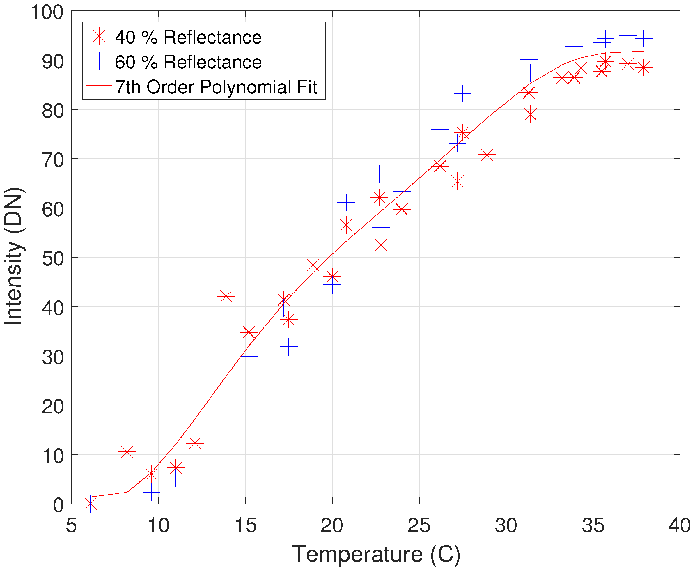
Figure 1 shows how the intensity changes with respect to the mean internal temperature of the Faro scanner. The intensity value obtained from the scanner has been referenced to the minimum intensity recorded for each target. This allows the change in intensity over temperature, of both the 40% and 60% target, to be compared to one another, irrespective of which target the data point was obtained from. From Figure 1, it is clear that the intensity of each target changes with a change in the internal temperature of the scanner, following a consistent relationship. A temperature correction was determined by fitting a seventh order polynomial to the data shown in Figure 1. A series of polynomials from the linear to 11th order were tested by applying them to data collected in Section 5.2. A 7th order polynomial was found to produce the best results and was selected.

The correction determined corrects the intensity to the intensity that would be received if the internal temperature were 40 ${}^{\circ }$C. The intensity correction can then be determined as

$$I_c=p\left(40\right)-p\left(T_m\right),$$

(6)

where $I_c$ is the intensity correction added to the received intensity, $p(·)$ is the fitted seventh order polynomial and $T_m$ is the mean temperature during the scan. In this research, the reflectance estimation method of Errington et al. [18] is used, but the temperature compensation can easily be applied to other methods, as it operates as an offset to the raw intensity value. It should be noted that, although this method can be easily applied with other radiometric correction methods, if other TLSs require temperature compensation, they too will have to be tested to determine their specific relationship between intensity and temperature.

5. Experiments

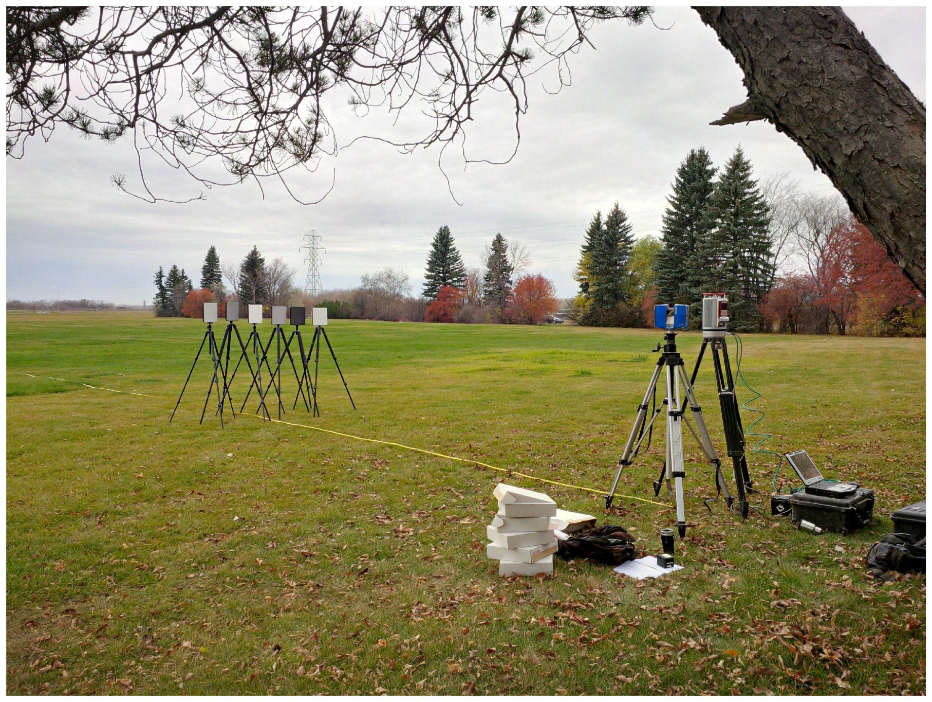
Three experiments for each instrument were conducted, both to determine the model parameters and to validate the generated models. In order to characterize the model, it is necessary to sample the intensity at various angles, positions and reflectances, as explained in Section 3. Figure 2 shows a photograph from one of the field tests where both the Riegl and Faro instrument were used simultaneously to collect data. Six Spectralon [24] calibrated diffuse reflectance targets were used in each experiment. Their nominal reflectances were 5%, 20%, 40%, 60%, 80% and 99%. The reflectance targets have slightly different reflectance values as compared to their nominal value. The reflectances at 1550 nm, the assumed wavelength for both scanners, are shown in

Table 1. Comparison of nominal and actual reflectances at 1550 nm, which is the wavelength of the two scanners, and each of the calibrated targets. This data was obtained from factory calibration data of the targets.

Nominal Reflectance	Actual Reflectance at 1550 nm
0.05	0.088
0.20	0.331
0.40	0.528
0.60	0.678
0.80	0.864
0.99	0.981

.

5.1. Riegl VZ-400

The Riegl VZ–400 is a pulse-based TLS which operates a laser of wavelength 1550 nm. It is a rugged device with passive cooling through its anodized aluminum housing. There were three experiments conducted using the VZ-400. The first two were conducted in a grass playing field (Field Test 1 and Field Test 2) during daylight and the third was conducted in a potash mine, which is approximately one kilometre underground (Allan mine), with no lighting present. The reasons for selecting these locations was twofold: (1) to see if different environmental conditions affect the resulting intensity, and (2) to provide multiple data sets to validate the model in different environments. This allows the model to be generated with a variety of data sets from different environments, in order to see how well it performs modelling alternative data sets. Note that the ambient air temperature of the field data sets was approximately 5 ${}^{\circ }$C and the underground mine data set was approximately 29 ${}^{\circ }$C.

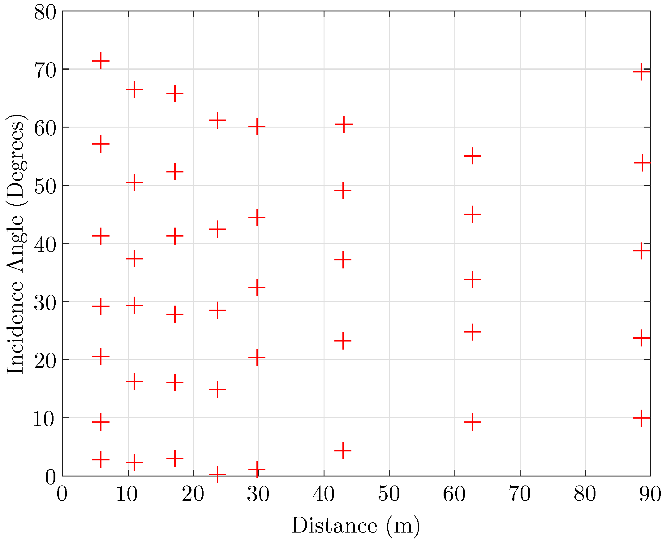
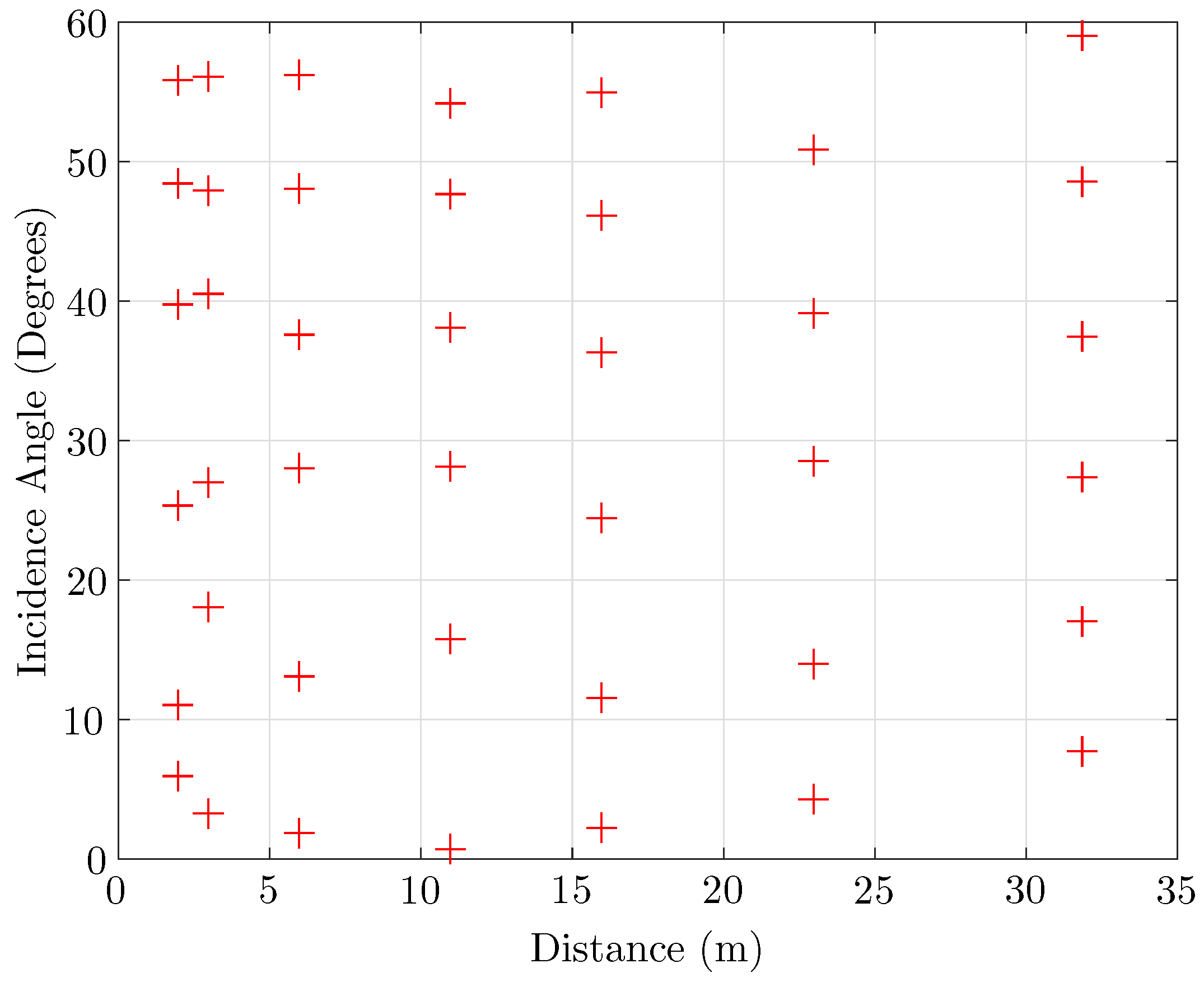
The sampling grid of the 5% reflectance target from the mine data set is shown in Figure 3. This figure illustrates at what distances and angles the 5% target was scanned. For example, at 30 m, the 5% target was scanned at approximately 5${}^{\circ }$, 23${}^{\circ }$, 37${}^{\circ }$, 49${}^{\circ }$ and 61${}^{\circ }$. This data was produced by placing the target at eight different distances from 5 m to 89 m. At each of these distances, the target was rotated to give incident angles between 0 to 72 degrees. The goal was to obtain consistent angular steps at each distance, and this was not always possible. For instance, at the distance of 89 m, for the 5% reflectance target, the lowest incidence angle achieved was 10${}^{\circ }$. This procedure was repeated for each of the reflectance targets. The average intensity over the whole target was used to obtain the data points shown in Figure 3. So, even though thousands of points land on the target, only the average value of those points is used in the model parametrization and verification. This same approach was used for the Faro instrument. It is important to note that the sampling grid shown in Figure 3 will be unique for each target and for each of the three experiments. In particular, Field Test 1 and the Allan Mine experiments were sampled at similar distance steps. However, Field Test 2 was sampled at distances $(2,3,5,7,10,14,20,30)$ m. The reason for differing spacing is to test the applicability of the radiometric correction in scenarios actually encountered.

5.2. Faro Focus${}^{3\mathrm{D}}$ X 330

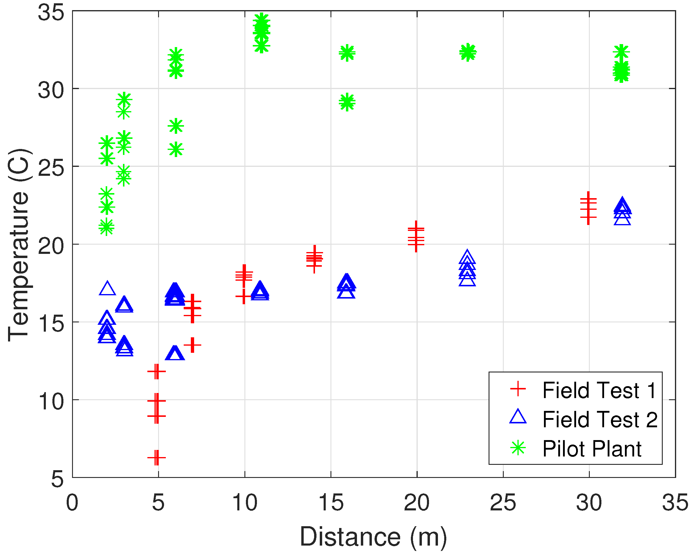
The Faro Focus${}^{3\mathrm{D}}$ X 330 is an Amplitude Modulated Continuous Wave (AMCW) phase–based scanner which operates at the same wavelength, 1550 nm, as the Riegl scanner. It is a fairly lightweight device with an integrated battery and utilizes active cooling through a recessed fan. Three data sets were collected for the Faro Focus${}^{3\mathrm{D}}$ X 330. Two data sets were collected in a grass playing field (Field Test 1 and Field Test 2) and one was collected in an industrial plant environment (Pilot Plant). The sampling grid for all three was quite similar and is shown in Figure 4. The ambient air temperature for the field data sets were approximately 5 ${}^{\circ }$C and the pilot plant data set was approximately 22 ${}^{\circ }$C.

Note, in Figure 4, that the angular sampling is never above 60 degrees. This was limited because, in the application of interest, the angle of incidence is kept well below this value. Similar to the Riegl tests, not all experiments were sampled at the same distances so that a true predictive error estimate could be obtained. For instance, Field Test 1 was sampled at distances of $(5,7,10,14,20,30)$.

5.3. Parameter Determination

As was discussed in Section 3, determining the model parameters is a two step process. The first step is to use Equation (4) at each of the distances sampled to estimate the parameters $p_1$ and $p_2$ at those distances. The results can be written in matrix form as in Equation (5). The second step fits a model, in this case a cubic spline, to each of the first and second columns of Equation (5). It is expected that this cubic spline model will perform well at, and between, the data points but not outside of the extents.

6. Results

The following subsections describe the results generated from the experiments for each individual instrument. The incidence angle is obtained by determining the best fit plane, in the least squares sense, to the 3D neighbourhood of points surronding the point of interest. The normal vector of the best fit plane is used to calculate the incidence angle. This procedure in described by Mitra and Nguyen [25].

6.1. Riegl VZ-400

Table 2. The error metrics for the three data sets. The model column was the data set used for generating the model parameters, whereas the Verification column was the data that the model was compared to that produced the error values, shown as standard deviation and mean error.

Data Set		Error
Model	Verification	St. Dev.	Mean
Allan Mine	Allan Mine	0.042	−0.001
Allan Mine	Field Test 1	0.060	0.017
Allan Mine	Field Test 2	0.045	0.041
Field Test 1	Field Test 1	0.053	0.021
Field Test 1	Field Test 2	0.046	0.046
Field Test 1	Allan Mine	0.041	0.004
Field Test 2	Field Test 2	0.052	0.010
Field Test 2	Allan Mine	0.053	−0.034
Field Test 2	Field Test 1	0.070	−0.049

presents the results of the reflectance estimation procedure applied to the three collected data sets. The table shows the error metrics for all combinations of model (training) and verification data sets. The rows in Table 2, which have the lowest error metrics are, of course, ones where the model and verification set are the same. In those cases, it is the model fit that is evaluated. In the other cases where the verification set is different, how well the generated model parameters perform on an independent data set is evaluated. It is also important to keep in mind that both Allan Mine and Field Test 1 data sets were sampled at approximately the same distances. This is reflected in the error results that show low error values involving these two data sets. In contrast, Field Test 2 was sampled at different distances from the other two data sets and the error values reflect this.

To better understand the error distribution, Figure 5 shows the results of using the Field Test 2 data set as both the model and verification sets. A more realistic example of the reflectance model’s performance is given in Figure 6, where the model is trained with the Field Test 2 data set and then this model is used with the Field Test 1 data set.

6.2. Faro Focus${}^{3\mathrm{D}}$ X 330

The need to compensate for the internal temperature of the scanner is demonstrated in Figure 7, which shows the mean internal temperature for the three data sets discussed in this section. More importantly, Figure 8 and Figure 9 show the error performance for the uncompensated and the temperature compensated reflectance estimate. In this case, the Pilot Plant data set was used to generate the model parameters and the model was applied to the Field Test 2 data set.

Table 3. A table showing the error metrics for the Faro instrument including both the Temperature compensated and the uncompensated reflectance estimate.

Data Set		Temperature Compensated Error		Uncompensated Error
Model	Verification	St. Dev.	Mean	St. Dev.	Mean
Pilot Plant	Pilot Plant	0.036	0.004	0.030	0.011
Pilot Plant	Field Test 1	0.063	−0.010	0.100	−0.128
Pilot Plant	Field Test 2	0.076	−0.056	0.104	−0.154
Field Test 1	Field Test 1	0.036	0.004	0.035	0.014
Field Test 1	Field Test 2	0.072	−0.040	0.082	−0.027
Field Test 1	Pilot Plant	0.072	0.030	0.100	0.142
Field Test 2	Field Test 2	0.037	0.005	0.034	0.015
Field Test 2	Pilot Plant	0.067	0.059	0.106	0.153
Field Test 2	Field Test 1	0.064	0.061	0.081	0.065

summarizes the error results when using/not using temperature compensation. The Model column specifies the data set that was used to parameterize the model while the Verification column specifies the data set that was used to compare the model with. Clearly, temperature compensation is not beneficial if the model and verification data set are the same. However, when verifying with the other two data sets, there is a clear improvement of the error performance. The largest improvement is in terms of the mean error performance.

7. Discussion

Table 4. A table showing the combined Root Mean Square (RMS) error metrics for the two scanners including both compensated and uncompensated Faro instrument. Displayed in the Error columns are the RMS errors of the standard deviation of the error and the RMS of the error (bias). Only those values where the verification data set is different from the model set are included in the mean.

Instrument	Error
	RMS St. Dev.	RMS Mean
Riegl VZ-400	0.053	0.032
Faro Focus${}^{3\mathrm{D}}$ X 330 Compensated	0.069	0.045
Faro Focus ${}^{3\mathrm{D}}$ X 330 Uncompensated	0.096	0.112

shows a summary of the results that can be used to compare the performance of the instruments and the reflectance estimation procedure. Displayed in the table are Root Mean Square (RMS) averages of the error metrics of the verification data sets, since these values are more representative of what one would expect to see in the acquired data. It is very clear from Table 4 that temperature compensation greatly improves the results for the Faro Focus${}^{3\mathrm{D}}$ X 330 instrument. The RMS of the mean error (displayed in the table as RMS Mean) improves by a factor of 2.6 while the RMS of the standard deviation of the error improves by a factor of 1.4. Importantly, without verification data sets to test the efficacy of the modeling procedure, it would not be possible to tell that this temperature correction was needed.

Although the temperature compensation of the Faro data reduces the error metrics, they are still larger than that for the Riegl instrument, which clearly does not require temperature compensation. It is unclear exactly why the Faro Focus${}^{3\mathrm{D}}$ X 330 requires compensation for temperature. However, it is clear, both from the experiments performed and the datasheets of the Spectralon reflectance targets [24], that the object’s reflectance is not changing. If this were the case, we would also see a discrepancy in the Riegl data. Additionally, in the temperature experiment, the intensity varied according to the scanner’s internal temperature and not directly with the ambient temperature. This points to internal instrument components being dependent upon temperature, such as the receiver amplifier stage. Without detailed proprietary information from the manufacturer, it is difficult to definitively show which components exhibit the temperature dependence. It may also be that the components used in the Riegl scanner do not have such a strong temperature dependence. It is also important to note that the scanners are fundamentally different in how they calculate range. The Riegl is a pulse-based scanner, whereas the Faro is a phase-based AMCW instrument.

A comparison to previous work is not trivial, but some of the most recent and applicable work is by Tan and Cheng [17] and Tan et al. [9]. In Refs. [9,17], the model for a Faro Focus${}^{3\mathrm{D}}$ X 330 was calibrated with diffuse reflectance targets and errors were presented. In fact, they provide a value of 0.0258 as the mean absolute error. If the same calculation is performed for the fit of the Pilot Plant data set (for both model and verification), a value of 0.0249 is obtained. However, this paper has limited the angle to be less than 60 degrees, whereas, in [17], it goes up to 80 degrees. However, the data set in this paper includes variation of the angle at each distance step, whereas, in [17], only a single angle series was considered. Furthermore, no verification of the reflectance targets was presented in [17], so it is not possible to tell whether their model ‘over fit’ the data. If a verification had been completed, without temperature compensation, poorer results would have been obtained, as was shown here.

From the work presented here, it should be clear that adequate verification data sets, in the varying environmental conditions in which they will be used, are necessary in determining expected prediction error as well as whether temperature compensation is necessary for a given TLS.

8. Conclusions

A method for modelling the reflectance of a diffuse surface using returned intensity, angle of incidence and range obtained from TLSs was verified. The reflectance modelling method was applied to two different TLS instruments: a Faro Focus${}^{3\mathrm{D}}$ X 330 and Riegl VZ-400. Overall, the VZ-400 produced better results with the RMS standard deviation of error being 0.053 and RMS of the mean error of 0.032. In the case of the Faro Focus${}^{3\mathrm{D}}$ X 330, it was found that the temperature of the instrument played an important role in the accuracy of the results. For this reason, a temperature compensation method was proposed that improved the RMS standard deviation of the error by 1.4 times and the RMS of the mean error by 2.4 times compared to the uncompensated results. This is the first time, to the best of the authors’ knowledge, that temperature compensation applied to intensity correction has appeared in the literature.

The results presented here also provide a verification of the model and the modelling process showing the model to be robust to environmental changes. However, as was shown for the Faro Focus${}^{3\mathrm{D}}$ X 330, some scanners may need additional corrections applied. The only way to determine the necessity of such corrections is to verify the models in disparate environments and conditions, as was performed in this paper.