Article

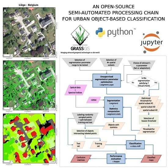
An Open-Source Semi-Automated Processing Chain for Urban Object-Based Classification

1
Department of Geoscience, Environment & Society, Université Libre De Bruxelles (ULB), 1050 Bruxelles, Belgium
2
Remote Sensing and Geodata Unit, Institut Scientifique de Service Public (ISSeP), 4000 Liège, Belgium
*
Author to whom correspondence should be addressed.
Remote Sens. 2017, 9(4), 358; https://doi.org/10.3390/rs9040358
Submission received: 19 December 2016 / Revised: 5 April 2017 / Accepted: 6 April 2017 / Published: 11 April 2017

Abstract

:
This study presents the development of a semi-automated processing chain for urban object-based land-cover and land-use classification. The processing chain is implemented in Python and relies on existing open-source software GRASS GIS and R. The complete tool chain is available in open access and is adaptable to specific user needs. For automation purposes, we developed two GRASS GIS add-ons enabling users (1) to optimize segmentation parameters in an unsupervised manner and (2) to classify remote sensing data using several individual machine learning classifiers or their prediction combinations through voting-schemes. We tested the performance of the processing chain using sub-metric multispectral and height data on two very different urban environments: Ouagadougou, Burkina Faso in sub-Saharan Africa and Liège, Belgium in Western Europe. Using a hierarchical classification scheme, the overall accuracy reached 93% at the first level (5 classes) and about 80% at the second level (11 and 9 classes, respectively).

Graphical Abstract

1. Introduction

Land-use/land-cover (LULC) information extraction is one of the main use cases of remote sensing imagery. The advent of sub-meter resolution data brought about the revolution of methods from pixel-based to object-based image analysis (OBIA) involving image segmentation. The latter provides many new opportunities and highly increases the quality of the output, but there remains a number of challenges to address.
First of all, segmentation parameters are often selected after a tedious and time-consuming trial-and-error refinement [1,2]. This method consists of a manual step-by-step segmentation parameters adjustment, relying on subjective visual human interpretation. Despite such efforts, the validity of the selected parameters is usually restricted to the specific scene under study, or even to specific areas within this scene, and they have to be adapted for each dataset. Unsupervised optimization methods meet the requirements for automation in the OBIA process, as they can be used to automatically adjust the segmentation parameters [1].
Second, during the classification step, many authors use rule-based approaches, which can be efficient on a specific dataset (e.g., [3,4]). However, their transferability remains an issue [5,6] as they also generally rely on manual intervention by the authors, with many choices guided by scene specificities. As an alternative, machine-learning classifiers, e.g., random forest or support vector machines (see [7,8] for a review of applications in remote sensing), have proven their efficiency for remote sensing data classification. While identification of the best performing classifier cannot rely on a priori knowledge, the combination of the results of multiple classifiers through an ensemble or voting schemes is a solution towards the development of more automated classification processes, as it “[...] makes the performance of the system more robust against the difficulties that each individual classifier may have on each particular data set”. [9] (p. 705).
Third, much of the work presented on OBIA tool chains is black box. First, the specific decisions of authors concerning parameter settings in the manual processes described above are based on their subjective evaluation, which is not always easy to reproduce. Moreover, even if their procedures are well documented, algorithms implemented in proprietary software cannot be properly reviewed as their code is distributed as closed source. This concerns the core software and also, in some cases, extensions of that software (e.g., the ‘Estimation of Scale Parameter’ (ESP) tool published in [10]). Furthermore, only those who have access to the software can attempt the replication of the results. In times when the reproducibility of research is high on the discussion agenda [11], the use of free and open-source solutions, including access to the code developed by researchers in their work, becomes paramount.
Linked to the previous point, the question of access to the necessary tools is of great importance, especially for many researchers in poorer countries where the lack of resources reduces their options [12], and especially for research using remote sensing [13]. Again, free and open-source solutions provide an answer to this issue by creating common-pool resources that all researchers can use, but also contribute to. Licensing costs can also be an obstacle to the upscaling of processes, especially in times of big data with ever-increasing spatial, spectral, and temporal resolutions [13]. Free and open-source software can help researchers surmount this challenge by letting them run their programs on as many different cores or machines as necessary without having to worry about software costs.
In this paper, we present a complete semi-automated processing chain for urban LULC mapping from earth observation data, which responds at least partly to the above issues. This chain was initially presented at the GEOBIA 2016 conference [14]. Freely available to any potential user, it should be seen as a framework that can be reused, modified, or enhanced for further studies. The chain was developed in a completely free and open-source environment, using GRASS GIS (Geographical Resources Analysis Support System) [15] and R [16], and was immediately reinjected into the wider open-source community. It contains tools for unsupervised segmentation parameter optimization, statistical characterization of objects, and machine-learning techniques combined through a majority-voting scheme. Care was taken to make the use of this processing chain accessible even to novice programmers. The proposed framework was tested with similar datasets on two very different urban environments to assess its transportability, i.e., the ability to achieve accurate classification when applying the same generic framework to different scenes with similar datasets [17].

2. Methods and Tools

The processing chain mainly relies on the open-source software GRASS GIS, that has been in continuous development since the 1980s and is now one of the core components of the Open Source Geospatial software stack [18]. This multipurpose Geographical Information System is made of hundreds of small programs [19], called ‘modules’ or ‘add-ons’, enabling users to carry out a large variety of geospatial processes [18]. Thanks to its continuous review mechanism and to its active community that has strong links with academia, GRASS GIS is increasingly being used by researchers [20,21,22,23,24,25]. Since 2012, GRASS GIS has had major advances in object-based image analysis (OBIA).
The proposed chain is made of the core Python code linking GRASS GIS functions thanks to the GRASS Python scripting library. It is implemented in a ‘Jupyter notebook’ that enables researchers to easily share the computer code that they developed for their studies and that often remains unpublished [26]. This programming environment allows users to mix both explanatory text sections with the related computer code that can be executed in the same document (see Figure 1). Care was taken to clearly document the code and to refer to the official help and/or scientific references. The Jupyter notebook is subdivided into several parts corresponding to the different processing steps (see Figure 1) which are summarized in the flowchart presented in Figure 2.
The GRASS GIS add-ons used in the processing chain are briefly presented below. For a more detailed description of those add-ons, interested readers may refer to the presentation made during the FOSS4G 2016 conference [27].

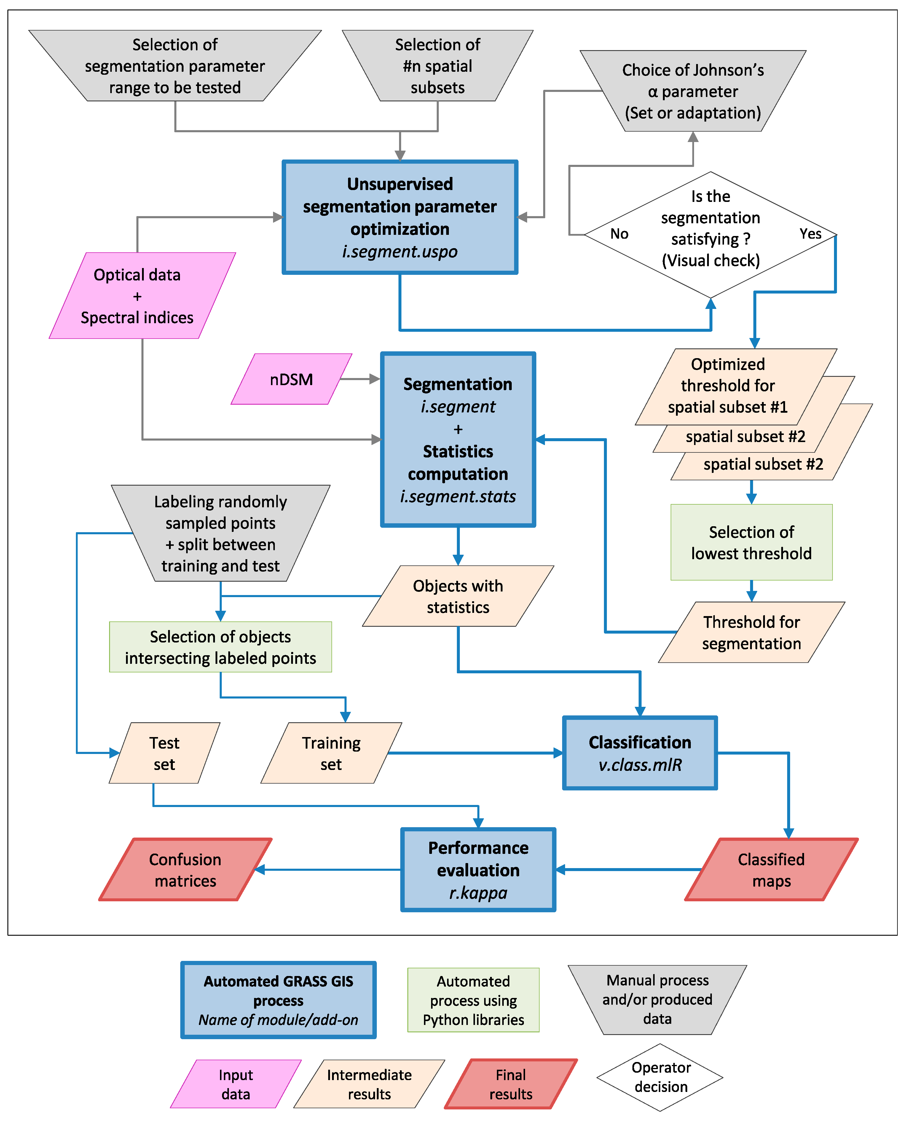
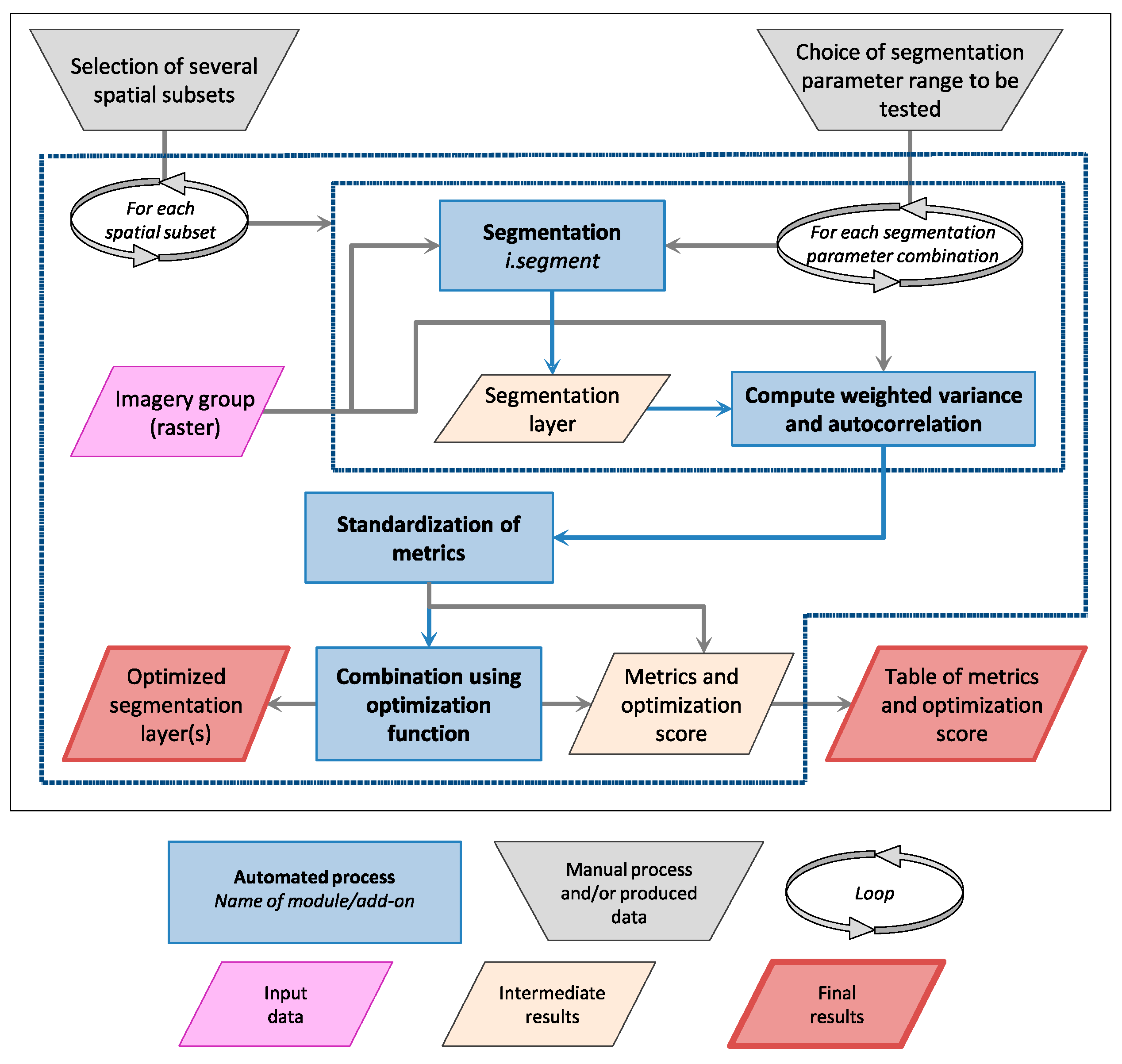
2.1. Segmentation and Unsupervised Segmentation Parameter Optimization (USPO) Tools

The segmentation was performed using the i.segment module of GRASS GIS [28]. This module implements image segmentation with a region-growing algorithm or an experimental mean-shift algorithm which was added recently. The region-growing algorithm, which is used in this study, requires a standardized ‘threshold’ parameter below which regions are merged, and a ‘minsize’ parameter defining the minimum size of regions. As with most GRASS GIS modules, the i.segment module is designed to handle very large datasets while keeping a low memory footprint. As an example of the orders of magnitudes, we encountered an issue when exceeding 2 billion objects, and this issue was solved quite quickly by the responsive GRASS Development Team. Most of the elements in the processing chain offer the option of using parallel computing to accelerate the analyses. Scaling is thus possible across all available cores, within the limits of available memory and input-output restrictions.
The choice of segmentation parameters is an important step in OBIA. Indeed, the ultimate goal of segmentation is to cluster individual pixels into meaningful objects, i.e., objects that correspond as much as possible to the geographical objects of interest in the scene. Moreover, the impact of segmentation quality on the accuracy of the classification seems obvious, even though a recent study [29] argues that this link is not so straightforward.
Usually, the selection of segmentation parameters is carried out using a ‘trial-and-error’ approach that relies on the visual assessment of several naïve segmentation results, and gradual adjustment of the segmentation parameters. This method presents the disadvantages of being subjective and requiring a tedious and time-consuming effort.
When objectivity is required in the evaluation of the segmentation results, several empirical methods can be used. Among them, a distinction can be made between the supervised (empirical discrepancy methods) and the unsupervised approaches (empirical goodness methods), depending on the requirement of a reference object delineation [1,30]. Both supervised and unsupervised methods allow the comparison of different segmentation algorithms or of different parameters used in a single algorithm (segmentation parameter optimization).
Supervised evaluation methods assess the divergence between a segmented image and a reference segmentation layer using ‘discrepancy measures’. Usually, the reference layer is created by delineating objects manually, thus requiring a time-consuming and highly subjective task.
In contrast, unsupervised evaluation methods assess the quality of a segmented image without the need of a reference or prior knowledge. This is the major advantage of these methods that can be used for automated segmentation parameter optimization [31]. Moreover, a recent study shows that they can achieve similar classification accuracy [32]. The evaluation relies on ‘goodness measures’ computed directly on the segmented image that represent the characteristics of a good segmentation. The uniformity of single objects (intra-segment homogeneity) and a significant difference between adjacent objects (inter-segment heterogeneity), firstly presented in [33] as desired characteristics of created objects, are now widely used in unsupervised evaluation methods. Several unsupervised approaches have been proposed in the literature, with different goodness measures and methods for combining them into a synthetic metric (see [1] for a review).
As we looked for automation, we elaborated a new GRASS GIS add-on for unsupervised segmentation parameter optimization (USPO) named i.segment.uspo [34]. Its working principle is illustrated on Figure 3. This tool is an implementation of the methods proposed by [31,35]. It relies on optimization functions combining measures of intra-object variance weighted by object size [32] (WV) as an intra-segment homogeneity quality measure, and spatial autocorrelation (SA) as an inter-segment heterogeneity quality measure [35]. For the latter, the user can choose between Moran’s I [36] or Geary’s C [37]. As the measure should be comparable for different segmentation results, both intra-segment homogeneity and inter-segment heterogeneity measures are normalized using the following function [35]:
F ( x ) = X m a x X X m a x X m i n
where F(x) is the normalized value of either WV or SA, X is the WV (or SA) value of the current segmentation result, and Xmax and Xmin are the maximum and minimum values of WV (or SA) for the whole stack of segmentation results to be evaluated. A high value for normalized WV (WVnorm) indicates higher undersegmentation, while a high value for normalized SA (SAnorm) highlights a higher oversegmentation.
The GRASS GIS add-on i.segment.uspo enables the combination of these WV and SA measures using two different optimization functions: a simple sum of the normalized criteria values as proposed by [35] or the F-function proposed by [31] that permits us to weight the two optimization criteria. The F-function is calculated as follows:
F = ( 1 + α 2 ) A S n o r m × W V n o r m α 2 × A S n o r m + W V n o r m
where F is the ‘overall goodness’, ranging from 0 (poor quality) to 1 (high quality) [31], to be used as a synthetic measure of the quality of the segmentation and α is a parameter that can be modified to give more weight to WV or to SA.
This overall goodness metric was designed in order to perform unsupervised segmentation parameter optimization for multi-scale OBIA (MS-OBIA) [31] (i.e., a process where different levels of segmentation are used together in the classification). In the semi-automated processing chain that was developed, the classification is performed using a single segmentation level. However, the chain could very easily be modified to enable MS-OBIA.
As highlighted in [38], the ability of USPO approaches to produce a good segmentation for specific features of interest in the scene is not straightforward, especially if those features are small-sized. Regarding this issue, we clearly recommend a visual check of the segmentation results to ensure that they are consistent with the objects of interest in the scene, as illustrated in the flowchart in Figure 2. If this is not the case, the α parameter in the Johnsons’ optimization function can be adapted to give more importance either to intra-segment homogeneity (set the α parameter higher than 1 to avoid residual undersegmentation) or to inter-segment heterogeneity (set the α parameter lower than 1 to avoid residual oversegmentation) [31]. More generally, it is clear that the ‘perfect’ segmentation does not exist [1,39,40], even if optimization methods are used. In their conclusion, Räsänen et al. argue that “[...] different segmentation evaluation methods should be used with care [...]. When segmentation evaluation is rigorously used, however, it can assist in finding a more optimal segmentation”. [29] (p. 8623).
Based on a range of parameter values provided by the user, the i.segment.uspo tool creates a set of segmentation results that are then assessed using the optimization function (see Figure 3). We suggest setting the range of segmentation parameter values to be tested by identifying values resulting in clearly under-segmented and over-segmented results, and using them as extremes. In order to reduce computation time during the optimization process, the tool provides the possibility to optimize the segmentation parameters on several spatial subsets of the scene (i.e., several zones limited in terms of area).
Care is recommended during the selection of those spatial subsets to ensure that they represent the diversity of the landscape that can be found in the whole scene. Detailed results are available (WV and AS measures and optimization scores for each segmentation parameter combination and each spatial subset), enabling the user to make an informed choice. Provided that there are no extreme outliers among the distribution of segmentation parameters from the different spatial subsets, the choice amongst the results can be completely automated by, for example, selecting the lowest value of the threshold parameter (as illustrated in Figure 2). Even though this approach could result in oversegmentation in some parts of the scene, some studies [39,41] argue that oversegmentation is preferable to undersegmentation, as the former can be corrected during classification, contrary to the latter. Furthermore, some recent studies [32,42] highlight that oversegmentation, as long as it remains at an admissible level, could be a minor issue in regard to the final classification result. Insofar that the different spatial subsets were well chosen to ensure that they represent the diversity of landscapes in the whole scene, the presence of extreme outliers among the optimized segmentation parameter is an indication that segmentation using a single parameter for the whole scene is not recommended. In this case, the whole scene could be subdivided into several more homogeneous areas according to some specific criteria. These areas could then be used as tiles in the segmentation workflow to perform local optimizations of the segmentation parameters [43].
The chain was designed to perform the segmentation process by dividing the scene using a vector layer provided by the user. This layer can consist of, e.g., arbitrary tiles or existing administrative boundaries. This implementation also allows users to manage very large datasets.

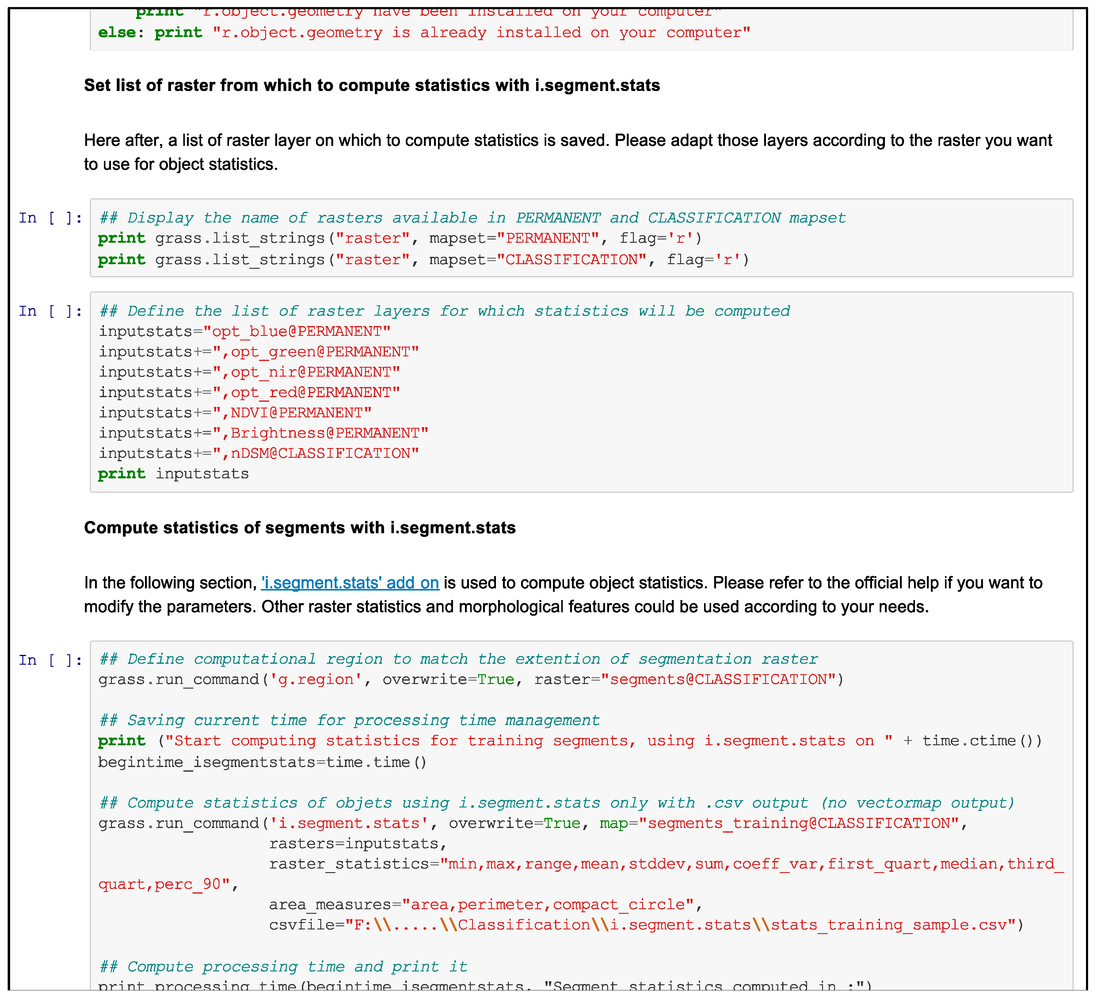
2.2. Object Statistics Computation

Object statistics were computed using the i.segment.stats GRASS GIS add-on [44] and were used as features in the classification process. This tool computes both the spectral statistics (e.g., min, max, median, stddev) and morphological statistics of objects (e.g., area, perimeter, compactness, fractal dimension). In order to speed up the calculation of the latter, another add-on, r.object.geometry [45], was developed. This add-on eliminates the need for vectorizing segments when computing morphological statistics, resulting in a significant gain in time.

2.3. Classification by the Combination of Multiple Machine Learning Classifiers

The classification stage of the processing chain uses the v.class.mlR GRASS GIS add-on [46]. It relies on the utilization of the “Caret” library of the R software [47], and enables the classification of data using Support Vector Machine (currently only with a radial kernel) (SVMradial), Random Forest (RF), Recursive partitioning (Rpart), and k-Nearest Neighbors (kNN) classifiers. This add-on automatically tunes classifiers’ parameters using repeated cross-validation with, by default, 10 iterations of 5-fold cross-validation on the training data set. Predictions of individual classifiers are then combined using several types of majority vote.
Four voting systems are provided: “Simple Majority Vote” (SMV), “Simple Weighted Vote” (SWV), “Best Worst Weighted Vote” (BWWV), and “Quadratic Best Worst Weighted Vote” (QBWWV). SMV simply consists of retaining the most frequent prediction. In the other votes, the predictions of individual classifiers are weighted. In SWV, the weight used is strictly the accuracy of individual classifiers estimated through cross-validation. In BWWV, the worst classifier is assigned a zero weight and is thereby not taken into account, and the best classifier is assigned a unit weight. The remaining classifiers are weighted linearly between 0 and 1. The last vote, QBWWV, is designed similarly to the former but the remaining classifiers are weighted using a squared function, amplifying the importance of more accurate classifiers. Interested readers can refer to [9] for the votes presented here and to [48] for more advanced methods used in remote sensing field.
A noticeable advantage of GRASS GIS is that it can be connected directly to R [16,49], allowing the exploitation of several advanced statistics methods (e.g., deep learning methods) implemented in this open-source software.

3. Case Studies

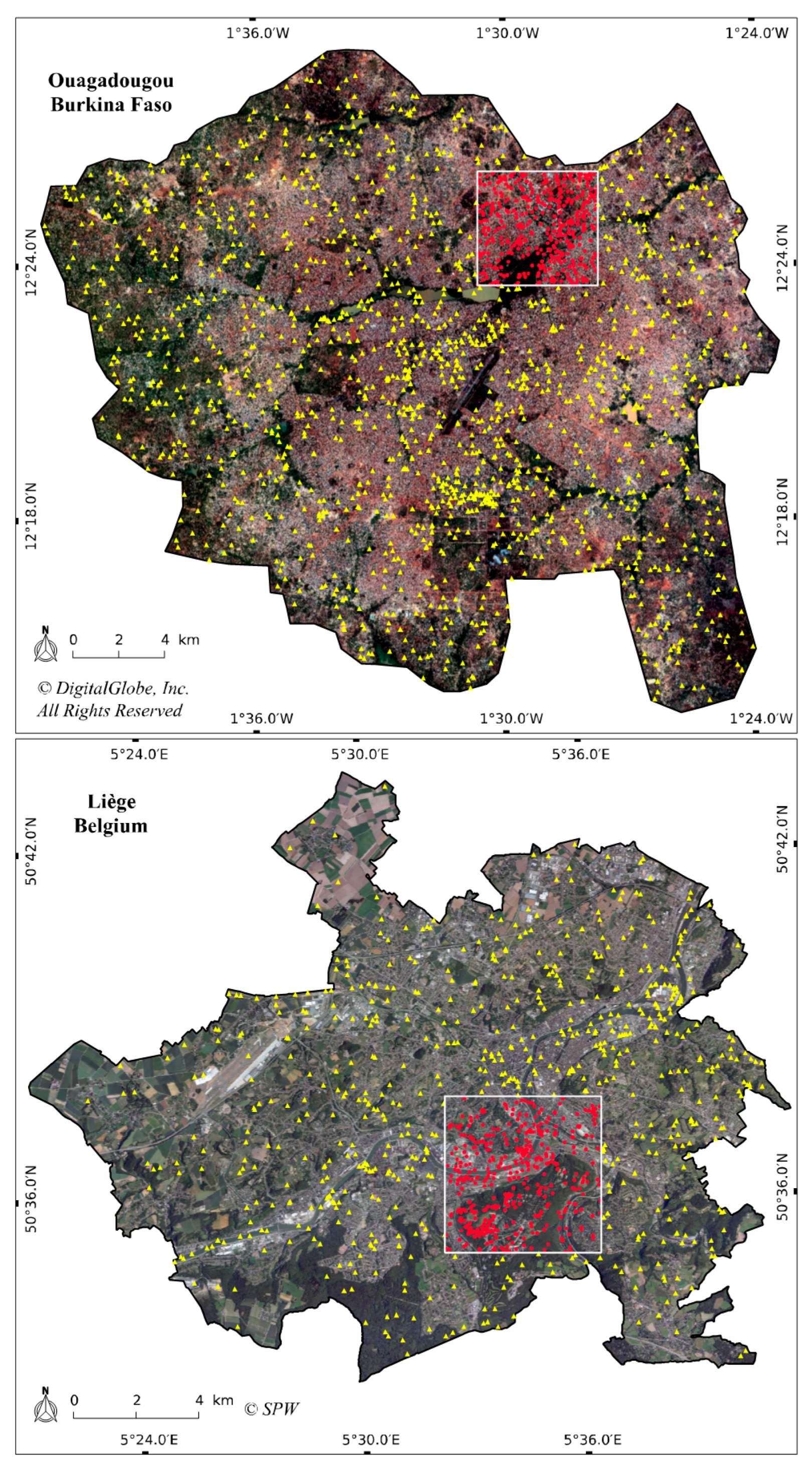
3.1. Study Areas and Data

In order to evaluate the transportability of the proposed processing chain, we applied it to two very different urban environments: Ouagadougou (Burkina Faso, in Sub-Saharan Africa) and Liège (Belgium, in Western Europe). More broadly, this work is linked with two research projects dealing with the production (Modelling and forecasting African Urban Population Patterns for vulnerability and health assessments project (MAUPP, http://maupp.ulb.ac.be/), focusing on African Sub-Saharan cities) and the update (SmartPop project, focusing on the Walloon region in Belgium, http://www.issep.be/smartpop/) of LULC maps. These maps will be used later as inputs in census population data disaggregation models.
The processing chain was first developed on Ouagadougou, the capital of Burkina Faso in Western Africa. Covering more than 615 km2, this city has been facing intensive urban sprawl during the last few decades similar to most sub-Saharan African cities and is characterized by very different urban patterns, such as planned versus unplanned residential areas, among others. Then, the processing chain was applied to the Liège area (261 km2), a Western European city located in Belgium which shows strong land artificialization (more than 55% of the territory). Urban morphologies are more diversified (from isolated houses to 10+ storey buildings), but urban sprawl is limited and controlled in comparison with Africa.
The datasets consist of multi-spectral and height data. For Ouagadougou, a pan sharpened stereo WorldView-3 imagery (Visible and Near-InfraRed bands (VNIR), spatial resolution of 0.5 m) acquired during the wet season (October 2015) and a normalized digital surface model (nDSM) (spatial resolution of 0.5 m) produced by stereophotogrammetry from WorldView-3 stereo-pairs were used. For Liège, the data consisted of leaf-on VNIR aerial orthophotos with a spatial resolution of 0.25 m acquired in May 2012 and a leaf-off nDSM extracted from Light Detection And Ranging data (LiDAR) (with a point density between 1 and 3 points per square meter) that was acquired in the winter of 2013–14.
As our processing chain is under development, we focused the classification effort on a 25 km2 subset for both cities (see Figure 4), representative of the diversity of landscapes and urban forms.

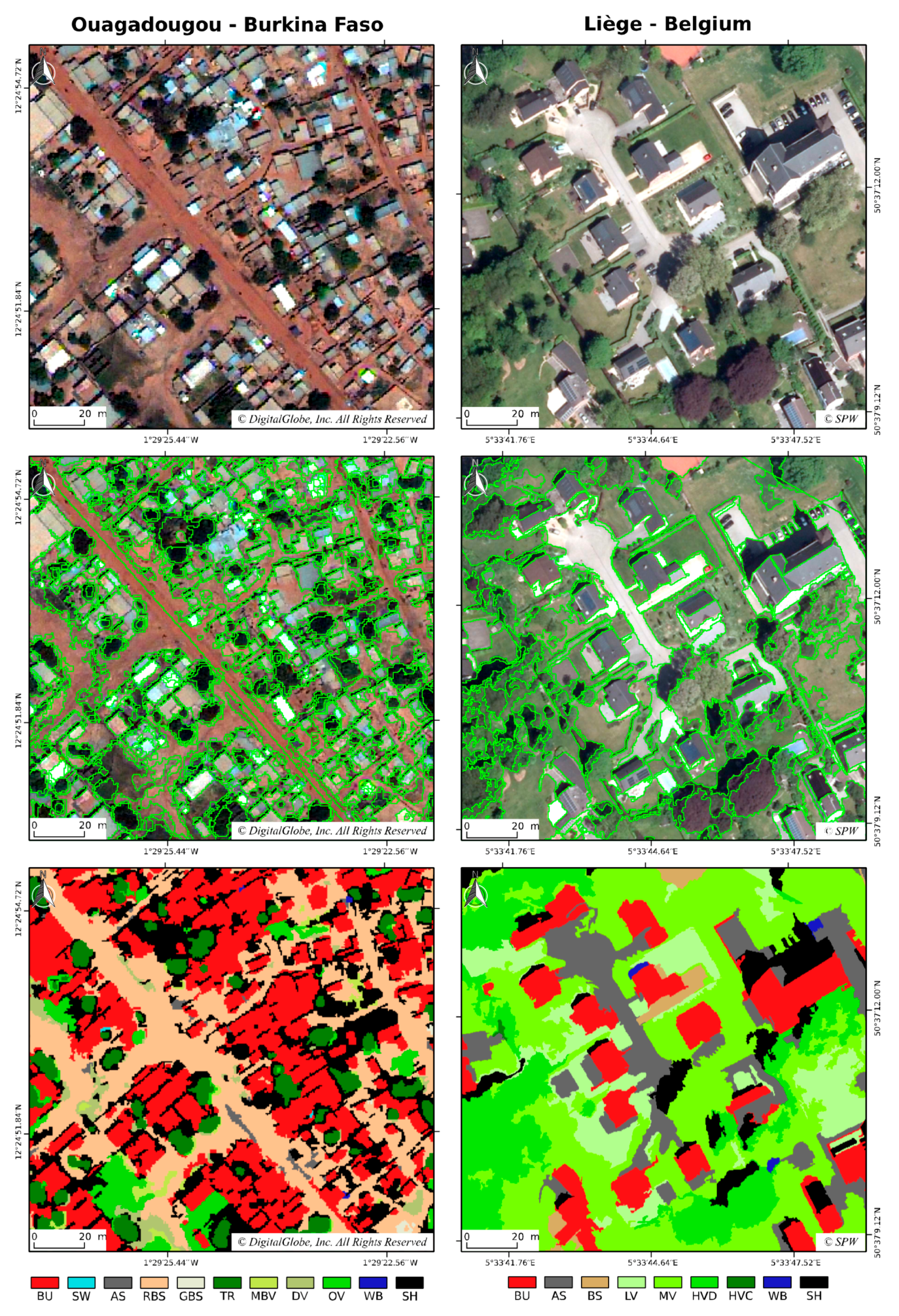
3.2. Legend/Classification Scheme

The classification scheme is organized in two hierarchical levels (see Table 1). The first level contains only land-cover (LC) classes, while the second level is a LULC mix of classes. At both levels, an extra class is dedicated to shadows; their post-processing is out of the scope of this article. The classification was made based on the second-level classes, which were aggregated to match the first-level classes.

3.3. Sampling Scheme

Sampling was conducted outside the processing chain, by generating random points and labelling them by hand, through visual image photo-interpretation. Although existing geodatabases were used for stratification, visual interpretation was needed to bypass thematic or spatial accuracy issues. In order to ensure a clear spatial independence, the training set was generated for the whole area excluding the 25 km2 subset where the classification was produced. An independent test set was generated inside this subset for performance evaluation purposes (see Figure 4). This procedure avoids potential spatial autocorrelation between the training and test sets.
For Ouagadougou, the OpenStreetMap (OSM) dataset was used as far as possible according to the availability. These data were used only for stratification purposes and only for some specific classes, i.e., for second-level classes of ‘buildings’, ‘asphalt surfaces’, and ‘water bodies’. When OSM datasets consisted of lines, as it is the case for asphalt roads and watercourses, buffers were created. Manual sampling was required for ‘swimming pools’ and ‘shadow’ classes. Intensive visual interpretation was needed for labelling each sampled point individually and to bypass mislabelled (cases where OSM attributes were false) and spatial inaccurate issues coming from the OSM data.
For Liège, existing official geodatabases from the national administration, i.e., ‘TOP10V’ (Institut Géographique National (IGN), 2010), and from the regional administration, i.e., ‘Projet Informatique de Cartographie Continue’ (PICC) (Service Public de Wallonie (SPW), 2007), were used for the stratification of the majority of second-level classes. Manual sampling was needed for the class ‘shadow’. Given the production date of the geodatabases used, a visual validation of the samples was needed to match the 2012/2013 land-cover status. In total, 1352 training points and 369 test points were created for Ouagadougou and 549 training points and 388 test points for Liège. The smaller size of the training set for Liège is explained by the reduced number of classes, their higher spectral consistency, and the intensive use of reference geodatabases. The class-distribution details are presented in Table 1.
Training and test points were used to automatically select intersecting segments and create the training and test sets. Although there is risk that some imperfect segments are used, the advantage of this strategy is that the same labelled set of points can be used with different segmentation results.

3.4. Segmentation

The segmentation and unsupervised segmentation parameter optimization (USPO) steps were carried out using multispectral information. For Ouagadougou, NDVI was also used as an additional layer. The nDSM layer was not used for the segmentation because of its insufficient geometric precision. The “minsize” parameter was set in order to match a chosen minimum mapping unit. The latter was defined according to the geographical context based on the smallest house/shelter: 2 m2 for Ouagadougou and 15 m2 for Liège. The intervention of the operator in the USPO process was limited to identification of the range of “threshold” parameters to be tested (minimum, maximum, and intervals), by manually looking for the thresholds resulting in clearly over-segmented or under-segmented objects. The optimized threshold was then automatically determined via the i.segment.uspo add-on. When giving the same weight to both intra-object homogeneity and inter-object heterogeneity measures (with the Johnson’s α parameter set to 1), objects of interest like small houses or trees were undersegmented. To avoid this issue, Johnson’s α parameter was then set to 1.25 for both Ouagadougou and Liège, in order to give more importance to intra-object homogeneity in the optimization function.

3.5. Classification Feature

For both case studies, the minimum, maximum, range, standard deviation, sum, and median statistics were computed for segments on the multispectral bands, NDVI and nDSM. These spectral statistics were completed with the morphological attributes of the objects (area, perimeter, and compactness).

4. Results

The classifications were performed at the second level of the legend scheme (see Table 1) using four individual machine learning classifiers that were combined using four voting systems. For each classification, the second-level classes were then aggregated to obtain the classes of the first level. The overall accuracy as well as Cohen’s Kappa metric of individual classifiers and vote combinations are presented in Table 2.
The ranking of individual classifiers’ performance is the same for Ouagadougou and Liège, with Random Forest (RF) performing best (overall accuracy (OA) of 81% and 79%, respectively), followed by Support Vector Machine with radial kernel (SVMradial) (75% and 74% OA, respectively), then Recursive partitioning (Rpart) (72% and 74% OA, respectively), and finally K–Nearest Neighbors classifier (kNN) (both 50% OA).
In the proposed processing chain, the training set is created by selecting the objects that contain the manually labelled point (see Figure 2), without any visual check. This design could result in the presence of mis-segmented objects in the training set which could perturb the classifiers. This explains why RF outperformed SVM, as studies show that RF is very robust when trained with imperfect data [50], while SVM is very sensitive to the presence of noise in the training set [51].
The user’s and producer’s accuracy computed on second-level classes are provided for each classification in Table A1 and Table A2. As assessing the performance with these measures can become very confusing, the F-score (harmonic mean of the user’s and producer’s accuracy) is used as a synthetic accuracy metric [52,53] in order to compare the classifiers’ performance on a class basis. The ‘buildings’ class is of particular importance in the context of the MAUPP and SmartPop projects since their final objective is to disaggregate census population data using LULC maps in order to model the spatial distribution of population densities. Using RF, this class reached a high accuracy for both case studies, with an F-score of 0.93 for Ouagadougou and 0.91 for Liège (see Table 3). For Ouagadougou, RF impressively outperformed Rpart and SVM for the class ‘buildings’ (both reaching an F-score of 0.78). This is also true for asphalt surfaces, with an F-score of 0.83 for RF, 0.61 for Rpart, and 0.55 for SVM. Again, those observations can be explained by the robustness of RF when dealing with imperfect data.
While satisfactory F-scores were obtained for specific classes such as ‘buildings’, ‘asphalt surfaces’, or ‘water bodies’, the accuracy is quite low for the other classes. It is also interesting to note that SVM and Rpart outperformed RF for specific classes in Ouagadougou (‘dry vegetation’ and ‘mixed bare soil/vegetation’, respectively).
The analysis of individual classifiers’ confusion matrices (see Table 4 and Table 5) revealed that, for both case studies, confusions occurred mainly between the different vegetation classes (46% and 61% of the whole confusions in Ouagadougou and Liège, respectively). In Ouagadougou, confusion also appeared between the bare soils classes (Brown/red bare soils; White/grey bare soils) and asphalt surfaces, shown in Table 4. Thanks to the hierarchical design of the legend, those confusions were greatly reduced when aggregating the second level classes to reach the first level of the legend. For this level, the overall accuracy is 93% for both case studies when considering the best performing voting scheme, i.e., the Simple Weighted Vote (SWV), shown in Table 2.
Despite the combination of individual predictions, majority votes do not perform better than the best individual classifier for the classes with high confusion, i.e., vegetation and bare soil classes. Conversely, the accuracy of other classes was improved by the votes. For example, it can be observed in Table 3 that the classes of ‘buildings’ and ‘bare soil’ benefit from the votes in Liège. The improvement resulting from the vote is more noticeable for the ‘other vegetation’ class in Ouagadougou, where the best-performing individual classifier (RF) reached an F-score of 0.77 while weighted votes (BWWV, QBWWV) reached 0.81. These balanced results, with votes outperforming individual classifiers for some classes and underperforming for others are consistent with the previous research [9]. The current method of attributing weight during the vote, using the overall accuracy of individual classifiers, is quite simple. Other methods might be implemented in order to take into account the performance of each classifier for specific classes (see [54] for a review of decision level fusion methods used in remote sensing).
Regarding segmentation, the use of an optimized segmentation parameter provided by i.segment.uspo achieved satisfactory results in our case studies. Even if the quantitative assessment of the segmentation’s quality is not in the scope of this paper, a visual check of Figure 5 reveals that the images are segmented into meaningful objects.
Even though a rigorous comparison of the results using different datasets and training/test sets could not be performed, the results obtained by applying the proposed semi-automated processing chain on two very different urban contexts are similar and attest the transportability of the proposed framework.

5. Discussion and Perspectives

The entire semi-automated processing chain for urban OBIA classification, relying on open-source solutions, is available on a dedicated Github repository (https://github.com/tgrippa/Opensource_OBIA_processing_chain). As it is shared under the CC-BY 4.0 Creative Common Licence, anyone interested can use and/or adapt it to match different project-specific needs, by integrating additional steps (e.g., automated image pre-processing, computation of spectral or textural indices, automated sampling based on existing reference geodatasets).
Other frameworks relying on open-source solutions have already been proposed for the extraction of valuable geographical information from remote sensing data [53,55,56,57,58]. Some of them are distributed as a plug-in or a toolbox for existing geographical information systems, mainly for QGIS [55,56,58], and present the advantage of providing a comforting environment for users, making their use quite simple.
For most of them, pixel-based image classification is their core task. However, some include basic object-based capabilities. For example, in the context of a pixel-based supervised classification, the Semi Automated Classification Plug-in (SACP) [55] enables the user to save time when creating regions of interest (ROI), as these are created using a region growing segmentation, starting from pixel seeds defined by the user. Another example is the ‘Twinned Object and Pixel-based Automated Classification chain‘ (TWOPAC) plug-in that enables performing classification using object-based derived features, but considers the segmentation as well as the object features computation as pre-processing steps to be performed outside of the tool [59].
After our investigations, we found only one existing open-source framework that allowed us to perform a complete object-based image analysis from segmentation to classification [57]. It relies fully on Python libraries and is a highly modular solution for object-based image analysis, as it can be linked with a lot of existing functions and software. Unfortunately, it could be very difficult for researchers without strong programming skills to handle this kind of framework.
In this paper, we propose a contribution toward the development of a fully automated processing chain for object-based image analysis. The advantage of the framework we propose is that it relies on the open-source software GRASS GIS, which has had recent enhancements for object-based image analysis, enabling the development of more automated procedures. As GRASS GIS offers a graphical user interface (GUI), the different commands can be tested in the GUI during the script development stage, and can then be included in the processing chain thanks to the GRASS Python scripting library. Another key advantage of GRASS GIS is its users’ and developers’ community, which is usually helpful and responsive.
Even though enhancements are desirable, the semi-automated processing chain currently achieved interesting results, as shown through the two case studies presented in this paper. Perspectives on further developments are discussed below in this section.
The generation of training and validation samples still requires strong manual expert intervention. This remains a challenge to be overcome by future research looking for automation, especially when highly accurate reference geodatabases are not available. In that case, alternative data such as OpenStreetMap data could be used, but their quality is often inconsistent and they should therefore be assessed prior to any automated use. Issues of co-registration with VHR imagery might also arise when using such data sets. The practical implementation of an active learning strategy [60], which could help in building efficient training sets more rapidly, is currently under development in GRASS GIS.
In order to improve the segmentation and hence the resulting classification, we intend to implement a multi-scale segmentation strategy, which has proved its ability to enhance the classification performance in a previous study [31]. Segmentation strategies using superpixels could also be investigated for further enhancements, since a new add-on [61] implementing SLIC superpixels method has been developed recently. This approach has provided interesting results in recent research [42].
Another improvement method concerns the features used as inputs in the classification process. Currently, only relatively simple object statistics are used. Band ratios and several textural indices will be added. They will be automatically computed and submitted to a feature selection procedure for those classifiers that do not include feature selection inherently.
During parameter tuning, spatial autocorrelation between the training and test sets created in cross-validation can lead to undetected overfitting and an overvaluation of the accuracy [62,63]. To reduce this potential bias and obtain better bootstrap error estimates, we will investigate the possibility of implementing spatial cross-validation, i.e., a spatially-constrained partitioning of the training and test sets created in cross-validation [64]. In addition, more classifiers will also be included.
Moreover, we will explore the possibility of implementing other strategies for the combination of multiple classifiers (see [48,54,65] for a review). The voting systems currently used to combine predictions are based on weights derived from the overall accuracy or kappa of individual classifiers, but in some cases, the non-best classifiers outperformed the best classifier's performance for specific classes (see Table 3).
Since the performance of different LULC mapping methods is currently being assessed in the SmartPop project, our open-source semi-automated approach is being compared to a rule-based approach, developed in a proprietary software. The latter integrates existing ancillary vector layers (buildings, roads, rails, and water bodies) in the segmentation. Constrained segmentation using ancillary vector layers in GRASS GIS will be investigated in future studies.
In the near future, the processing chain will be tested on different datasets and/or cities. For the MAUPP project, Synthetic Aperture Radar (SAR) data will be added as an input in order to improve the accuracy and the chain will be applied to Ouagadougou (Burkina Faso), Dakar, and Saint-Louis (Senegal). For the SmartPop project, Pléiades imagery will be used instead of orthophotos in order to assess the comparative advantage of each dataset. Thereafter, the efficiency of the processing chain will be tested for the automated processing of a very large area (i.e., the Walloon Region in Belgium), taking advantage of the parallel computing options in the different modules.

6. Conclusions

In times when the reproducibility of research and the sharing of existing solutions is high on the discussion agenda, the development of free and open-source solutions becomes paramount. In this paper, a semi-automated processing chain for urban object-based classification is proposed as a contribution towards the development of a transparent and open-source fully automated processing chain for urban land-use/land-cover mapping from earth observation data. This processing chain, relying on existing open-source geospatial software, is very adaptable and transportable to similar datasets. It proved its ability of being quickly customizable in order to match the requirements of different projects, with very different urban morphologies and different datasets. Freely available for anyone interested, it should be seen as a framework to be reused and enhanced for further studies. The results achieved on our case studies are very interesting, taking into account the complexity of the urban environments and the detail of the legend.

Acknowledgments

This work was funded by the Belgian Federal Science Policy Office (BELSPO) (Research Program for Earth Observation STEREO III, contract SR/00/304—as part of the MAUPP project—http://maupp.ulb.ac.be) and by the Moerman research program of ISSeP (SmartPop project—http://www.issep.be/smartpop). The add-on ’v.class.mlR’ was based on a initial work of Ruben Van De Kerchove who is acknowledged for his contribution. Service Public de Wallonie (SPW) is acknowledged for providing aerial orthophotos, LiDAR, and ancillary vector geodatabases (LIC 160128-1348, all rights reserved to SPW). WorldView3 data is copyrighted under the mention “©COPYRIGHT 2015 DigitalGlobe, Inc., Longmont CO USA 80503. DigitalGlobe and the DigitalGlobe logos are trademarks of DigitalGlobe, Inc. The use and/or dissemination of this data and/or of any product in any way derived there from are restricted. Unauthorized use and/or dissemination is prohibited”. OpenStreetMap data are copyrighted under the mention “©OpenStreetMap contributors, CC BY-SA”. The authors greatly thank the reviewers for their relevant comments which helped to improve this manuscript.

Author Contributions

Taïs Grippa, Moritz Lennert, Benjamin Beaumont, and Sabine Vanhuysse wrote the manuscript. Taïs Grippa is the main author who developed the processing chain and applied it on both case studies. Moritz Lennert implemented the new GRASS GIS add-ons and provided precious technical support. Benjamin Beaumont and Sabine Vanhuysse created the training and test sets. Nathalie Stephenne and Eléonore Wolff contributed actively to the revisions of the manuscript.

Conflicts of Interest

The authors declare no conflict of interest.

Appendix A

Table A1. Performance evaluation of the level-2 classification of Ouagadougou, Burkina Faso. Producer accuracy (PA) and User accuracy (UA) for each class of the second level of classification. For each line, the highest value is in bold. BU: Buildings. SW: Swimming pools. AS: Asphalt surfaces. RBS: Brown/red bare soil. GBS: White/grey bare soil. TR: Trees. MBV: Mixed bare soil/vegetation. DV: Dry vegetation. OV: Other vegetation. WB: Water bodies. SH: Shadow.
Individual ClassifiersVotes
Level 2 ClassesAccuracykNNRpartSVMradialRFSMVSWVBWWVQBWWV
BUPA:79.1%79.1%100.0%95.3%97.7%97.7%95.3%95.3%
UA:51.5%77.3%64.2%91.1%76.4%89.4%89.1%89.1%
SWPA:83.9%87.1%93.5%96.8%96.8%96.8%96.8%96.8%
UA:100.0%96.4%100.0%100.0%100.0%100.0%100.0%100.0%
ASPA:56.7%83.3%56.7%90.0%86.7%90.0%90.0%90.0%
UA:44.7%48.1%53.1%77.1%74.3%77.1%77.1%77.1%
RBSPA:57.1%83.3%64.3%85.7%85.7%85.7%85.7%85.7%
UA:47.1%68.6%65.9%72.0%69.2%70.6%70.6%70.6%
GBSPA:26.7%56.7%56.7%56.7%50.0%53.3%53.3%53.3%
UA:25.0%89.5%94.4%100.0%93.8%100.0%100.0%100.0%
TRPA:50.0%96.9%81.3%90.6%90.6%90.6%90.6%90.6%
UA:69.6%72.1%83.9%80.6%74.4%78.4%80.6%80.6%
MBVPA:28.1%62.5%46.9%46.9%50.0%50.0%50.0%50.0%
UA:30.0%60.6%78.9%68.2%66.7%69.6%69.6%69.6%
DVPA:6.3%46.9%71.9%62.5%65.6%65.6%65.6%65.6%
UA:12.5%50.0%59.0%58.8%61.8%60.0%58.3%58.3%
OVPA:63.9%61.1%72.2%80.6%69.4%77.8%80.6%80.6%
UA:48.9%84.6%74.3%74.4%80.6%77.8%80.6%80.6%
WBPA:12.9%64.5%80.6%83.9%64.5%80.6%80.6%80.6%
UA:36.4%87.0%89.3%89.7%90.9%89.3%89.3%89.3%
SHPA:73.3%60.0%93.3%96.7%96.7%96.7%96.7%96.7%
UA:75.9%90.0%93.3%90.6%93.5%93.5%90.6%90.6%
OA50,1%71.5%74.8%81.0%78.3%81.0%81.0%81.0%
Kappa0.450.690.720.790.760.790.790.79
Table A2. Performance evaluation of the level-2 classification of Liège, Belgium. Producer accuracy (PA) and User accuracy (UA) for each class of the second level of classification. For each line, the highest value is in bold. BU: Buildings. AS: Asphalt surfaces. LV: Low vegetation (<1 m). MV: Medium vegetation (1–7 m). HVD: High vegetation deciduous (>7 m). HVC: High vegetation coniferous (>7 m). BS: Bare soil. WB: Water bodies. SH: Shadow.
Individual ClassifiersVotes
Level 2 ClassesAccuracykNNRpartSVMradialRFSMVSWVBWWVQBWWV
BUPA:48.6%89.2%81.1%86.5%91.9%89.2%86.5%86.5%
UA:52.9%94.3%85.7%97.0%94.4%97.1%97.0%97.0%
ASPA:78.3%70.0%76.7%78.3%81.7%80.0%80.0%80.0%
UA:54.7%72.4%76.7%85.5%75.4%84.2%84.2%84.2%
LVPA:32.6%69.6%65.2%78.3%78.3%71.7%71.7%71.7%
UA:42.9%86.5%76.9%81.8%81.8%82.5%82.5%82.5%
MVPA:33.3%68.8%58.3%64.6%62.5%64.6%64.6%64.6%
UA:34.8%66.0%66.7%73.8%73.2%68.9%68.9%68.9%
HVDPA:33.3%72.2%75.0%75.0%75.0%75.0%75.0%75.0%
UA:25.0%53.1%49.1%54.0%50.0%52.9%52.9%52.9%
HVCPA:34.9%74.4%62.8%72.1%65.1%72.1%72.1%72.1%
UA:37.5%69.6%71.1%73.8%71.8%73.8%73.8%73.8%
BSPA:40.5%61.9%69.0%76.2%57.1%73.8%73.8%73.8%
UA:60.7%65.0%72.5%72.7%77.4%75.6%73.8%73.8%
WBPA:73.0%97.3%91.9%94.6%94.6%94.6%94.6%94.6%
UA:90.0%81.8%91.9%100.0%100.0%100.0%100.0%100.0%
SHPA:71.8%69.2%92.3%94.9%94.9%94.9%94.9%94.9%
UA:68.3%93.1%85.7%86.0%86.0%86.0%86.0%86.0%
OA50.3%74.0%74.0%79.4%77.3%78.9%78.6%78.6%
Kappa0.440.710.710.770.740.760.760.76

References

  1. Zhang, H.; Fritts, J.E.; Goldman, S.A. Image segmentation evaluation: A survey of unsupervised methods. Comput. Vis. Image Underst. 2008, 110, 260–280. [Google Scholar] [CrossRef]
  2. Blaschke, T. Object based image analysis for remote sensing. ISPRS J. Photogramm. Remote Sens. 2010, 65, 2–16. [Google Scholar] [CrossRef]
  3. Salehi, B.; Zhang, Y.; Zhong, M.; Dey, V. Object-Based Classification of Urban Areas Using VHR Imagery and Height Points Ancillary Data. Remote Sens. 2012, 4, 2256–2276. [Google Scholar] [CrossRef]
  4. O’Neil-Dunne, J.P.M.; MacFaden, S.W.; Royar, A.R.; Pelletier, K.C. An object-based system for LiDAR data fusion and feature extraction. Geocarto Int. 2013, 28, 227–242. [Google Scholar] [CrossRef]
  5. Kohli, D.; Warwadekar, P.; Kerle, N.; Sliuzas, R.; Stein, A. Transferability of Object-Oriented Image Analysis Methods for Slum Identification. Remote Sens. 2013, 5, 4209–4228. [Google Scholar] [CrossRef]
  6. Belgiu, M.; Drǎguţ, L.; Strobl, J. Quantitative evaluation of variations in rule-based classifications of land cover in urban neighbourhoods using WorldView-2 imagery. ISPRS J. Photogramm. Remote Sens. 2014, 87, 205–215. [Google Scholar] [CrossRef] [PubMed]
  7. Mountrakis, G.; Im, J.; Ogole, C. Support vector machines in remote sensing: A review. ISPRS J. Photogramm. Remote Sens. 2011, 66, 247–259. [Google Scholar] [CrossRef]
  8. Belgiu, M.; Drăgut, L. Random forest in remote sensing: A review of applications and future directions. ISPRS J. Photogramm. Remote Sens. 2016, 114, 24–31. [Google Scholar] [CrossRef]
  9. Moreno-Seco, F.; Inesta, J.M.; De León, P.J.P.; Micó, L. Comparison of classifier fusion methods for classification in pattern recognition tasks. In Joint IAPR International Workshops on Statistical Techniques in Pattern Recognition (SPR) and Structural and Syntactic Pattern Recognition; Springer: Berlin/Heidelberg, Germany, 2006; pp. 705–713. [Google Scholar]
  10. Drăguţ, L.; Csillik, O.; Eisank, C.; Tiede, D. Automated parameterisation for multi-scale image segmentation on multiple layers. ISPRS J. Photogramm. Remote Sens. 2014, 88, 119–127. [Google Scholar] [CrossRef] [PubMed]
  11. Skaggs, T.H.; Young, M.H.; Vrugt, J.A. Reproducible Research in Vadose Zone Sciences. Vadose Zone J. 2015, 14. [Google Scholar] [CrossRef]
  12. Walsham, G.; Sahay, S. Research on information systems in developing countries: Current landscape and future prospects. Inf. Technol. Dev. 2006, 12, 7–24. [Google Scholar] [CrossRef]
  13. Haack, B.; Ryerson, R. Improving remote sensing research and education in developing countries: Approaches and recommendations. Int. J. Appl. Earth Obs. Geoinf. 2016, 45, 77–83. [Google Scholar] [CrossRef]
  14. Grippa, T.; Lennert, M.; Beaumont, B.; Vanhuysse, S.; Stephenne, N.; Wolff, E. An open-source semi-automated processing chain for urban obia classification. In Proceedings of the GEOBIA 2016: Solutions and Synergies, Enschede, The Netherlands, 14–16 September 2016. [Google Scholar]
  15. GRASS Development Team. Geographic Resources Analysis Support System (GRASS). Open Source Geospatial Foundation: Chicago, IL, USA, 2015. Available online: https://grass.osgeo.org/ (accessed on 13 June 2016).
  16. R Development Core Team. R: A Language and Environment for Statistical Computing; R Foundation for Statistical Computing: Vienna, Austria, 2008. [Google Scholar]
  17. Walker, J.S.; Blaschke, T. Object-based land-cover classification for the Phoenix metropolitan area: Optimization vs. transportability. Int. J. Remote Sens. 2008, 29, 2021–2040. [Google Scholar] [CrossRef]
  18. Neteler, M.; Bowman, M.H.; Landa, M.; Metz, M. GRASS GIS: A multi-purpose open source GIS. Environ. Model. Softw. 2012, 31, 124–130. [Google Scholar] [CrossRef]
  19. Neteler, M.; Beaudette, D.E.; Cavallini, P.; Lami, L.; Cepicky, J. Grass gis. In Open Source Approaches in Spatial Data Handling; Springer: Berlin/Heidelberg, Germany, 2008; pp. 171–199. [Google Scholar]
  20. Hofierka, J.; Kaňuk, J. Assessment of photovoltaic potential in urban areas using open-source solar radiation tools. Renew. Energy 2009, 34, 2206–2214. [Google Scholar] [CrossRef]
  21. Frigeri, A.; Hare, T.; Neteler, M.; Coradini, A.; Federico, C.; Orosei, R. A working environment for digital planetary data processing and mapping using ISIS and GRASS GIS. Planet. Space Sci. 2011, 59, 1265–1272. [Google Scholar] [CrossRef]
  22. Sofina, N.; Ehlers, M. Object-based change detection using highresolution remotely sensed data and gis. In Proceedings of the International Archives Photogrammetry, Remote Sensing and Spatial Information Sciences-XXII ISPRS Congress, Melbourne, Australia, 25 August–1 September 2012; Volume 39, p. B7. [Google Scholar]
  23. Rocchini, D.; Delucchi, L.; Bacaro, G.; Cavallini, P.; Feilhauer, H.; Foody, G.M.; He, K.S.; Nagendra, H.; Porta, C.; Ricotta, C.; et al. Calculating landscape diversity with information-theory based indices: A GRASS GIS solution. Ecol. Inform. 2013, 17, 82–93. [Google Scholar] [CrossRef]
  24. Do, T.H.; Raghavan, V.; Vinayaraj, P.; Truong, X.L.; Yonezawa, G. Pixel Based and Object Based Fuzzy LULC Classification using GRASS GIS and RapidEye Imagery of Lao Cai Area, Vietnam. Geoinformatics 2016, 27, 104–105. [Google Scholar]
  25. Petrasova, A.; Mitasova, H.; Petras, V.; Jeziorska, J. Fusion of high-resolution DEMs for water flow modeling. Open Geospatial Data Softw. Stand. 2017, 2, 6. [Google Scholar] [CrossRef]
  26. Kluyver, T.; Ragan-Kelley, B.; Pérez, F.; Granger, B.; Bussonnier, M.; Frederic, J.; Kelley, K.; Hamrick, J.; Grout, J.; Corlay, S.; et al. Jupyter Notebooks—A publishing format for reproducible computational workflows. In Positioning and Power in Academic Publishing: Players, Agents and Agendas; IOS Press: Amsterdam, The Netherlands, 2016; pp. 87–90. [Google Scholar]
  27. Lennert, M. A Complete Toolchain for Object-Based Image Analysis with GRASS GIS 2016. Available online: http://video.foss4g.org/foss4g2016/videos/index.html (accessed on 25 November 2016).
  28. Momsen, E.; Metz, M.; GRASS Development Team Module i.segment. Geographic Resources Analysis Support System (GRASS) Software, Version 7.3; Open Source Geospatial Foundation: Chicago, IL, USA, 2015. Available online: https://grass.osgeo.org/grass73/manuals/i.segment.html (accessed on 25 November 2016).
  29. Räsänen, A.; Rusanen, A.; Kuitunen, M.; Lensu, A. What makes segmentation good? A case study in boreal forest habitat mapping. Int. J. Remote Sens. 2013, 34, 8603–8627. [Google Scholar] [CrossRef]
  30. Zhang, Y.J. A survey on evaluation methods for image segmentation. Pattern Recognit. 1996, 29, 1335–1346. [Google Scholar] [CrossRef]
  31. Johnson, B.A.; Bragais, M.; Endo, I.; Magcale-Macandog, D.B.; Macandog, P.B.M. Image Segmentation Parameter Optimization Considering Within- and Between-Segment Heterogeneity at Multiple Scale Levels: Test Case for Mapping Residential Areas Using Landsat Imagery. ISPRS Int. J. Geo-Inf. 2015, 4, 2292–2305. [Google Scholar] [CrossRef]
  32. Belgiu, M.; Drăgut, L. Comparing supervised and unsupervised multiresolution segmentation approaches for extracting buildings from very high resolution imagery. ISPRS J. Photogramm. Remote Sens. 2014, 96, 67–75. [Google Scholar] [CrossRef] [PubMed]
  33. Haralick, R.M.; Shapiro, L.G. Image segmentation techniques. Comput. Vis. Graph. Image Process. 1985, 29, 100–132. [Google Scholar] [CrossRef]
  34. Lennert, M.; GRASS Development Team Addon i.segment.uspo. Geographic Resources Analysis Support System (GRASS) Software, Version 7.3; Open Source Geospatial Foundation: Chicago, IL, USA, 2016. Available online: https://grass.osgeo.org/grass70/manuals/addons/i.segment.uspo.html (accessed on 25 November 2016).
  35. Espindola, G.M.; Camara, G.; Reis, I.A.; Bins, L.S.; Monteiro, A.M. Parameter selection for region-growing image segmentation algorithms using spatial autocorrelation. Int. J. Remote Sens. 2006, 27, 3035–3040. [Google Scholar] [CrossRef]
  36. Moran, P.A.P. Notes on Continuous Stochastic Phenomena. Biometrika 1950, 37, 17–23. [Google Scholar] [CrossRef] [PubMed]
  37. Geary, R.C. The Contiguity Ratio and Statistical Mapping. Inc. Stat. 1954, 5, 115–145. [Google Scholar] [CrossRef]
  38. Grybas, H.; Melendy, L.; Congalton, R.G. A comparison of unsupervised segmentation parameter optimization approaches using moderate- and high-resolution imagery. GISci. Remote Sens. 2017, 0, 1–19. [Google Scholar] [CrossRef]
  39. Carleer, A.P.; Debeir, O.; Wolff, E. Assessment of very high spatial resolution satellite image segmentations. Photogramm. Eng. Remote Sens. 2005, 71, 1285–1294. [Google Scholar] [CrossRef]
  40. Johnson, B.; Xie, Z. Unsupervised image segmentation evaluation and refinement using a multi-scale approach. ISPRS J. Photogramm. Remote Sens. 2011, 66, 473–483. [Google Scholar] [CrossRef]
  41. Schiewe, J. Segmentation of high-resolution remotely sensed data-concepts, applications and problems. Int. Arch. Photogramm. Remote Sens. Spat. Inf. Sci. 2002, 34, 380–385. [Google Scholar]
  42. Csillik, O. Fast Segmentation and Classification of Very High Resolution Remote Sensing Data Using SLIC Superpixels. Remote Sens. 2017, 9, 243. [Google Scholar] [CrossRef]
  43. Cánovas-García, F.; Alonso-Sarría, F. A local approach to optimize the scale parameter in multiresolution segmentation for multispectral imagery. Geocarto Int. 2015, 30, 937–961. [Google Scholar] [CrossRef]
  44. Lennert, M.; GRASS Development Team Addon i.segment.stats. Geographic Resources Analysis Support System (GRASS) Software, Version 7.3; Open Source Geospatial Foundation: Chicago, IL, USA, 2016. Available online: https://grass.osgeo.org/grass70/manuals/addons/i.segment.stats.html (accessed on 25 November 2016).
  45. Metz, M.; Lennert, M.; GRASS Development Team Addon r.object.geometry. Geographic Resources Analysis Support System (GRASS) Software, Version 7.3; Open Source Geospatial Foundation: Chicago, IL, USA, 2016. Available online: https://grass.osgeo.org/grass72/manuals/addons/r.object.geometry.html (accessed on 25 November 2016).
  46. Lennert, M.; GRASS Development Team Addon v.class.mlR. Geographic Resources Analysis Support System (GRASS) Software, Version 7.3; Open Source Geospatial Foundation: Chicago, IL, USA, 2016. Available online: https://grass.osgeo.org/grass70/manuals/addons/v.class.mlR.html (accessed on 25 November 2016).
  47. Kuhn, M. Building Predictive Models in R Using the caret Package. J. Stat. Softw. 2008, 28, 115571. [Google Scholar] [CrossRef]
  48. Du, P.; Xia, J.; Zhang, W.; Tan, K.; Liu, Y.; Liu, S. Multiple Classifier System for Remote Sensing Image Classification: A Review. Sensors 2012, 12, 4764–4792. [Google Scholar] [CrossRef] [PubMed]
  49. Neteler, M.; Mitasova, H. Open Source GIS—A GRASS GIS Approach. Available online: http://link.springer.com.ezproxy.ulb.ac.be/book/10.1007%2F978-0-387-68574-8 (accessed 2 November 2014).
  50. Folleco, A.; Khoshgoftaar, T.M.; Hulse, J.V.; Bullard, L. Identifying Learners Robust to Low Quality Data. In Proceedings of the 2008 IEEE International Conference on Information Reuse and Integration, Las Vegas, NV, USA, 13–15 July 2008; pp. 190–195. [Google Scholar]
  51. Foody, G.; Pal, M.; Rocchini, D.; Garzon-Lopez, C.; Bastin, L. The Sensitivity of Mapping Methods to Reference Data Quality: Training Supervised Image Classifications with Imperfect Reference Data. ISPRS Int. J. Geo-Inf. 2016, 5, 199. [Google Scholar] [CrossRef]
  52. Sokolova, M.; Lapalme, G. A systematic analysis of performance measures for classification tasks. Inf. Process. Manag. 2009, 45, 427–437. [Google Scholar] [CrossRef]
  53. Inglada, J.; Vincent, A.; Arias, M.; Tardy, B.; Morin, D.; Rodes, I. Operational High Resolution Land Cover Map Production at the Country Scale Using Satellite Image Time Series. Remote Sens. 2017, 9, 95. [Google Scholar] [CrossRef]
  54. Zeng, Y.; Zhang, J.; Van Genderen, J.L. Comparison and Analysis of Remote Sensing Data Fusion Techniques at Feature and Decision Levels. In Proceedings of the ISPRS Commission VII Mid-term Symposium Remote Sensing: From Pixels to Processes, Enschede, The Netherlands, 8–11 May 2006. [Google Scholar]
  55. Congedo, L. Semi-Automatic Classification Plugin User Manual, Release 5.3.6.1; RoMEO: Paterson, NJ, USA, 2017. [Google Scholar]
  56. Huth, J.; Kuenzer, C.; Wehrmann, T.; Gebhardt, S.; Tuan, V.Q.; Dech, S. Land Cover and Land Use Classification with TWOPAC: Towards Automated Processing for Pixel- and Object-Based Image Classification. Remote Sens. 2012, 4, 2530–2553. [Google Scholar] [CrossRef]
  57. Clewley, D.; Bunting, P.; Shepherd, J.; Gillingham, S.; Flood, N.; Dymond, J.; Lucas, R.; Armston, J.; Moghaddam, M. A Python-Based Open Source System for Geographic Object-Based Image Analysis (GEOBIA) Utilizing Raster Attribute Tables. Remote Sens. 2014, 6, 6111–6135. [Google Scholar] [CrossRef]
  58. Guzinski, R.; Kass, S.; Huber, S.; Bauer-Gottwein, P.; Jensen, I.; Naeimi, V.; Doubkova, M.; Walli, A.; Tottrup, C. Enabling the Use of Earth Observation Data for Integrated Water Resource Management in Africa with the Water Observation and Information System. Remote Sens. 2014, 6, 7819–7839. [Google Scholar] [CrossRef]
  59. Huth, J.; Kuenzer, C. TWOPAC Handbook: Twinned Object and Pixel-Based Automated Classification Chain; RoMEO: Paterson, NJ, USA, 2013. [Google Scholar]
  60. Tuia, D.; Volpi, M.; Copa, L.; Kanevski, M.; Munoz-Mari, J. A Survey of Active Learning Algorithms for Supervised Remote Sensing Image Classification. IEEE J. Sel. Top. Signal Process. 2011, 5, 606–617. [Google Scholar] [CrossRef]
  61. Kanavath, R.; Metz, M.; GRASS Development Team Addon i.superpixels.slic. Geographic Resources Analysis Support System (GRASS) Software, Version 7.3; Open Source Geospatial Foundation: Chicago, IL, USA, 2017. Available online: https://grass.osgeo.org/grass72/manuals/addons/i.superpixels.slic.html (accessed on 20 February 2017).
  62. Mannel, S.; Price, M.; Hua, D. Impact of reference datasets and autocorrelation on classification accuracy. Int. J. Remote Sens. 2011, 32, 5321–5330. [Google Scholar] [CrossRef]
  63. Brenning, A. Spatial Cross-Validation and Bootstrap for the Assessment of Prediction Rules in Remote Sensing: The R Package Sperrorest. In Proceedings of the 2012 IEEE International Geoscience and Remote Sensing Symposium, Munich, Germany, 22–27 July 2012; pp. 5372–5375. [Google Scholar]
  64. Brenning, A.; Long, S.; Fieguth, P. Detecting rock glacier flow structures using Gabor filters and IKONOS imagery. Remote Sens. Environ. 2012, 125, 227–237. [Google Scholar] [CrossRef]
  65. Lisini, G.; Dell’Acqua, F.; Trianni, G.; Gamba, P. Comparison and Combination of Multiband Classifiers for Landsat Urban Land Cover Mapping. In Proceedings of the 2005 IEEE International Geoscience and Remote Sensing Symposium, Seoul, Korea, 25–29 July 2005; Volume 4, pp. 2823–2826. [Google Scholar]
Figure 1. Excerpt of the “Jupyter notebook” consisting of a sequence of descriptive text parts that document the different processing steps and cells of the Python script that can be executed directly from the notebook.
Remotesensing 09 00358 g001
Figure 2. Flowchart of the processing chain.
Remotesensing 09 00358 g002
Figure 3. Selection of the optimized thresholds by i.segment.uspo.
Remotesensing 09 00358 g003
Figure 4. Ouagadougou and Liège case studies. True color composite is used as the background. For both cities, the classification was made on the white-squared subset. Training samples are in yellow while the test samples are in red.
Remotesensing 09 00358 g004
Figure 5. True color composite (top), results of segmentation with Unsupervised Segmentation Parameter Optimization USPO (middle), classification at the second level with SWV vote (bottom) on a subset for each case study. BU: Buildings, SW: Swimming pools, AS: Asphalt surfaces, BS: Bare soil, RBS: Brown/red bare soil, GBS: White/grey bare soil, TR: Tree, MBV: Mixed bare soil/vegetation, DV: Dry vegetation, LV: Low vegetation, MV: Medium vegetation, HVD: High vegetation deciduous, HVD: High vegetation coniferous, OV: Other vegetation, WB: Water bodies, SH: Shadow.
Remotesensing 09 00358 g005
Table 1. Classification scheme and size of the training and test sets for Ouagadougou and Liège.
Level 1 Classes
Land Cover (LC)
Level 2 Classes
Land Use/Land Cover (LULC)
AbbreviationTraining Set SizeTest Set Size
Ouagadougou–Burkina Faso
Artificial surfacesBuildingsBU21643
Swimming poolsSW9031
Asphalt surfacesAS11930
Natural material surfacesBrown/red bare soilRBS13042
White/grey bare soilGBS9130
VegetationTreesTR9132
Mixed bare soil/vegetationMBV9932
Dry vegetationDV9332
Other vegetationOV21836
WaterWater bodiesWB11531
ShadowShadowSH9030
Liège–Belgium
Artificial surfacesBuildingsBU6237
Asphalt surfacesAS8660
Natural material surfacesBare soilBS5142
VegetationLow vegetation (<1 m)LV5546
Medium vegetation (1–7 m)MV4948
High vegetation deciduous (>7 m)HVD6336
High vegetation coniferous (>7 m)HVC4943
WaterWater bodiesWB7237
ShadowShadowSH6239
Table 2. Performance evaluation of individual classifiers and the four different voting systems. For each line, the highest value is in bold. OA: Overall accuracy. L1 and L2: Levels of the classification scheme. kNN: k-Nearest Neighbors. Rpart: Recursive partitioning. SVMradial: Support Vector Machine with radial kernel. RF: Random Forest. SMV: Simple Majority Vote. SWV: Simple Weighted Vote. BWWV: Best Worst Weighted Vote. QBWWV: Quadratic Best Worst Weighted Vote.
Individual ClassifiersVotes
kNNRpartSVMradialRFSMVBWWVQBWWVSWV
OuagadougouL1Kappa0.690.800.840.900.870.900.900.90
OA77%85%88%93%91%92%92%93%
L2Kappa0.450.690.720.790.760.790.790.79
OA50%72%75%81%78%81%81%81%
LiègeL1Kappa0.750.830.870.890.880.890.890.89
OA82%88%90%92%91%92%92%93%
L2Kappa0.440.710.710.770.740.760.760.76
OA50%74%74%79%77%79%79%79%
Table 3. F-score for individual classes for the second level (L2) of the classification. For each line, the highest value is in bold. kNN: k-Nearest Neighbors. Rpart: Recursive partitioning. SVMradial: Support Vector Machine with radial kernel. RF: Random Forest. SMV: Simple Majority Vote. SWV: Simple Weighted Vote. BWWV: Best Worst Weighted Vote. QBWWV: Quadratic Best Worst Weighted Vote.
Individual ClassifiersVotes
Level 2 ClasseskNNRpartSVMradialRFSMVSWVBWWVQBWWV
Ouagadougou–Burkina Faso
Buildings0.620.780.780.930.860.930.920.92
Swimming pools0.910.920.970.980.980.980.980.98
Asphalt surfaces0.500.610.550.830.800.830.830.83
Brown/red bare soil0.520.750.650.780.770.770.770.77
White/grey bare soil0.260.690.710.720.650.700.700.70
Trees0.580.830.830.850.820.840.850.85
Mixed bare soil/vegetation0.290.620.590.560.570.580.580.58
Dry vegetation0.080.480.650.610.640.630.620.62
Other vegetation0.550.710.730.770.750.780.810.81
Inland waters0.190.740.850.870.750.850.850.85
Shadow0.750.720.930.940.950.950.940.94
Liège–Belgium
Buildings0.510.920.830.910.930.930.910.91
Asphalt surfaces0.640.710.770.820.780.820.820.82
Low vegetation (<1 m)0.370.770.710.800.800.770.770.77
Medium vegetation (1–7 m)0.340.670.620.690.670.670.670.67
High vegetation deciduous (>7 m)0.290.610.590.630.600.620.620.62
High vegetation coniferous (>7 m)0.360.720.670.730.680.730.730.73
Bare soil0.490.630.710.740.660.750.740.74
Inland waters0.810.890.920.970.970.970.970.97
Shadow0.700.790.890.900.900.900.900.90
Table 4. Confusion matrix for the Simple Weighted Vote on Ouagadougou, Burkina Faso. Values are given as a percentage of the reference test set (column-based normalization). Diagonal values correspond to the producer accuracy. BU: Buildings, SW: Swimming pools, AS: Asphalt surfaces, RBS: Brown/red bare soil, GBS: White/grey bare soil, TR: Tree, MBV: Mixed bare soil/vegetation, DV: Dry vegetation, OV: Other vegetation, WB: Water bodies, SH: Shadow.
Reference
L2 ClassesBUSWASRBSGBSTRMBVDVOVWBSH
Simple Weighted Vote (SWV)BU97.70006.6700009.680
SW096.8000000000
AS009011.90009.38000
RBS003.3385.736.706.25003.230
GBS000053.3000000
TR0000090.603.1319.400
MBV2.33002.383.3305012.5000
DV00000040.665.62.7800
OV000009.383.136.2577.83.233.33
WB006.6700003.13080.60
SH03.2300000003.2396.7
Table 5. Confusion matrix for the Simple Weighted Vote on Liège, Belgium. Values are given as a percentage of the reference test set (column-based normalization). Diagonal values correspond to the producer accuracy. BU: Buildings, AS: Asphalt surfaces, LV: Low vegetation, MV: Medium vegetation, HVD: High vegetation deciduous, HVD: High vegetation coniferous, BS: Bare soil, WB: Water bodies, SH: Shadow.
Reference
L2 ClassesBUASLVMVHVDHVCBSWBSH
Simple Weighted Vote (SWV)BU89.21.670000000
AS5.4180000016.700
LV0071.78.33007.1400
MV0028.364.6002.3800
HVD000257527.9000
HVC0002.0822.272.1005.13
BS2.715000073.800
WB000000094.60
SH2.73.33002.78005.4194.9

