
In-Field High-Throughput Phenotyping of Cotton Plant Height Using LiDAR


Abstract
:
1. Introduction
2. Materials and Methods
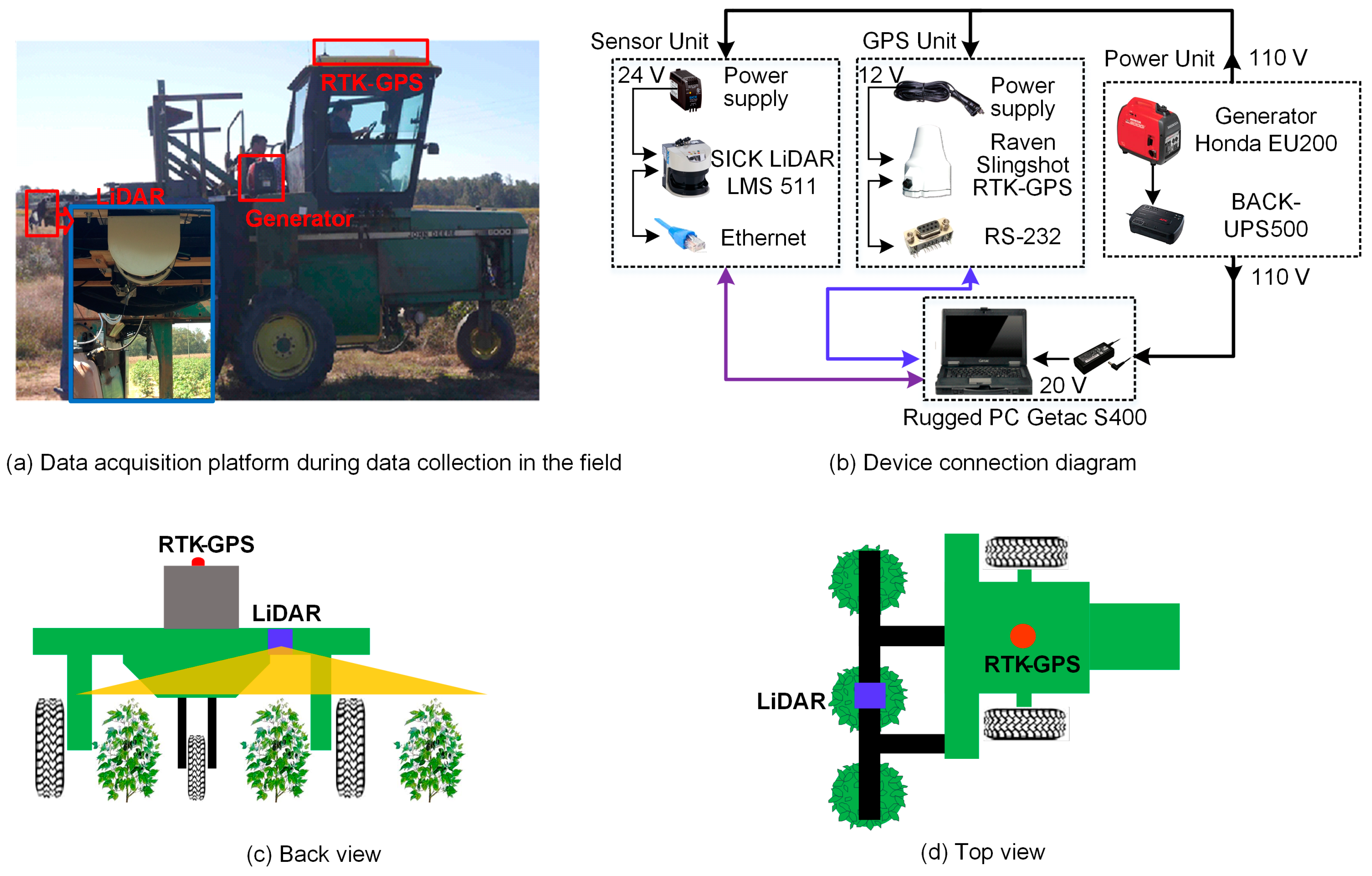
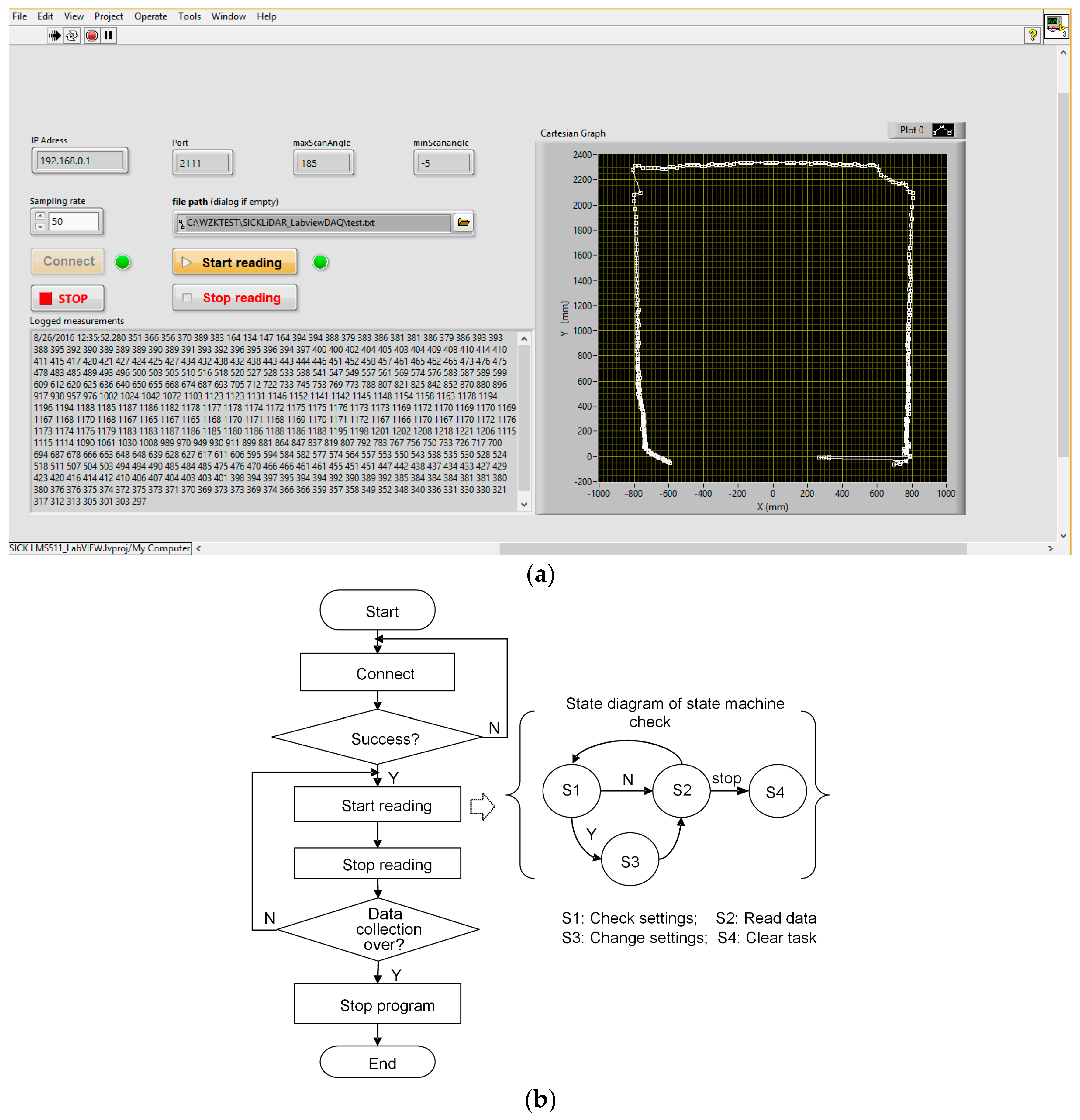
2.1. Data Acquisition System
2.2. Configuration of System Parameters
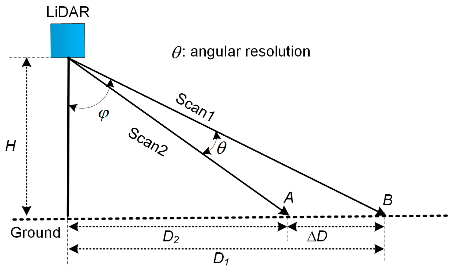
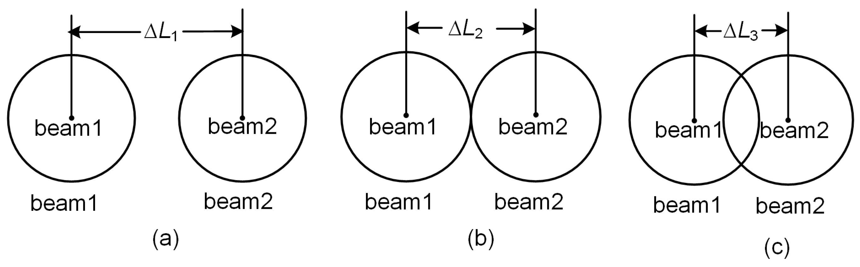
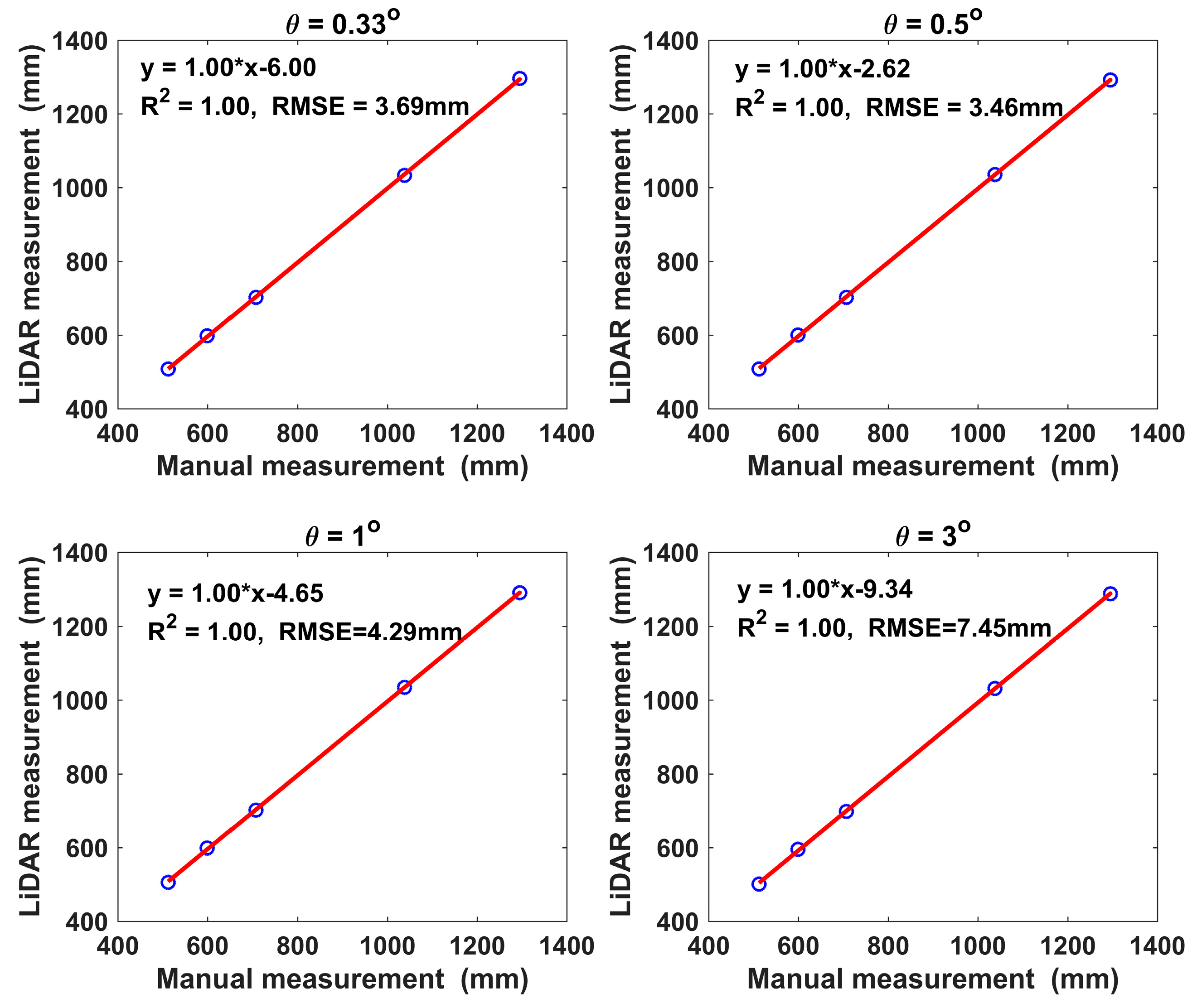
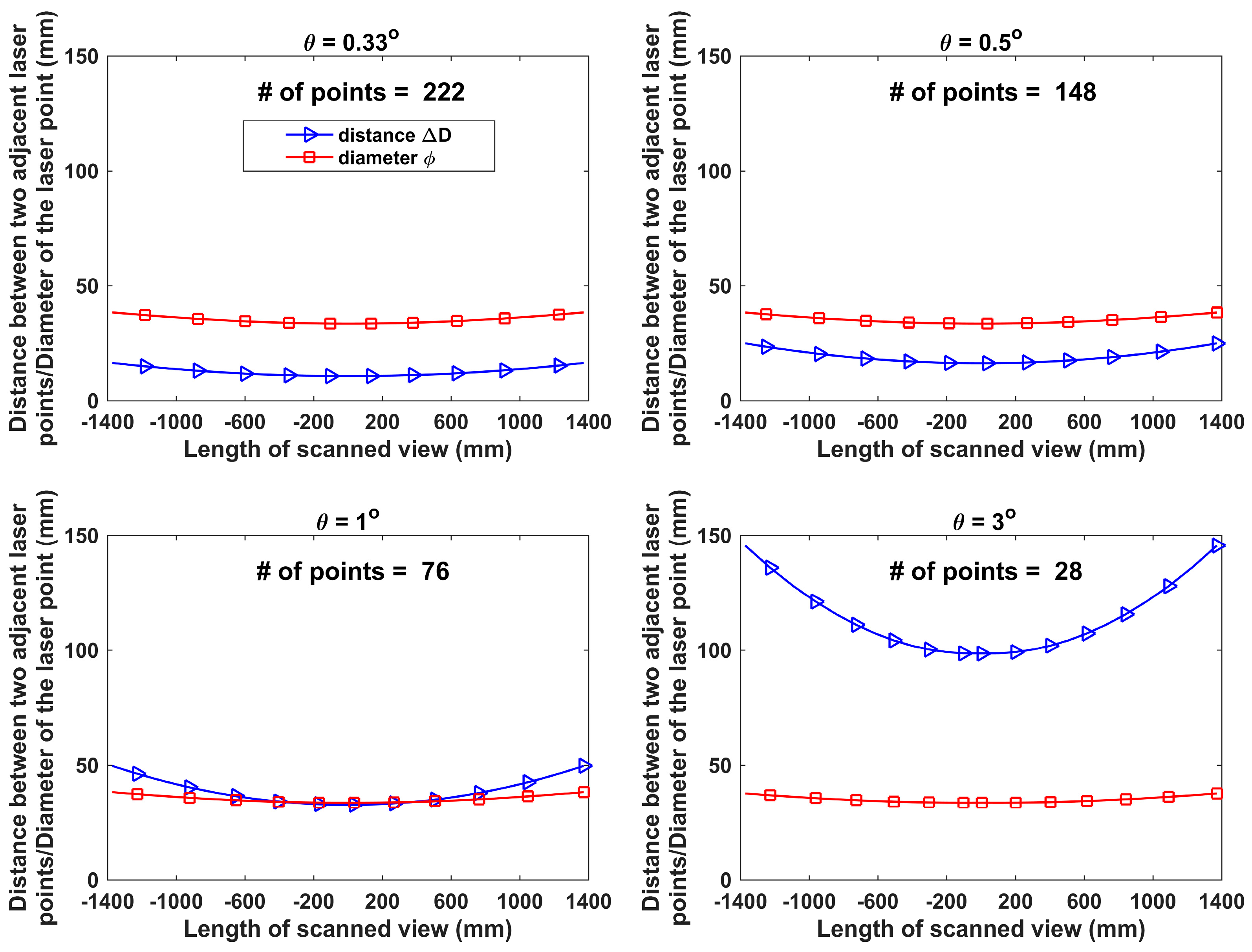
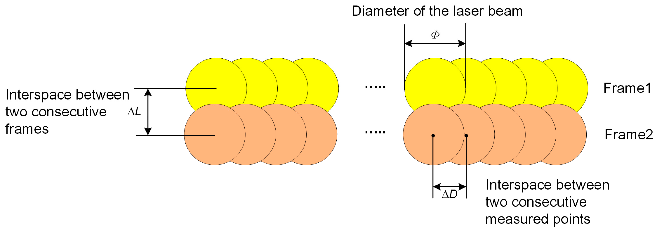
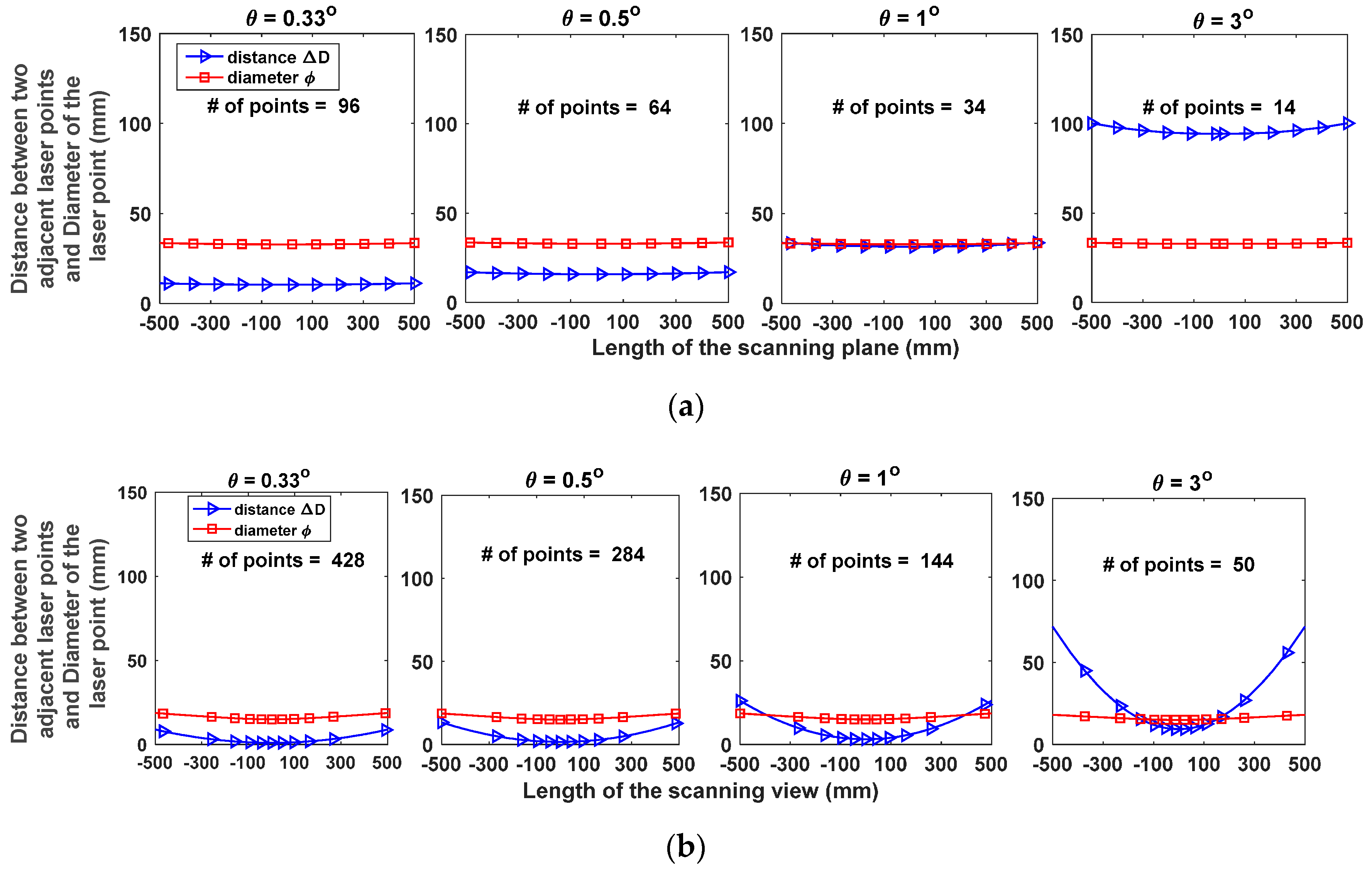
2.2.1. Angular Resolution
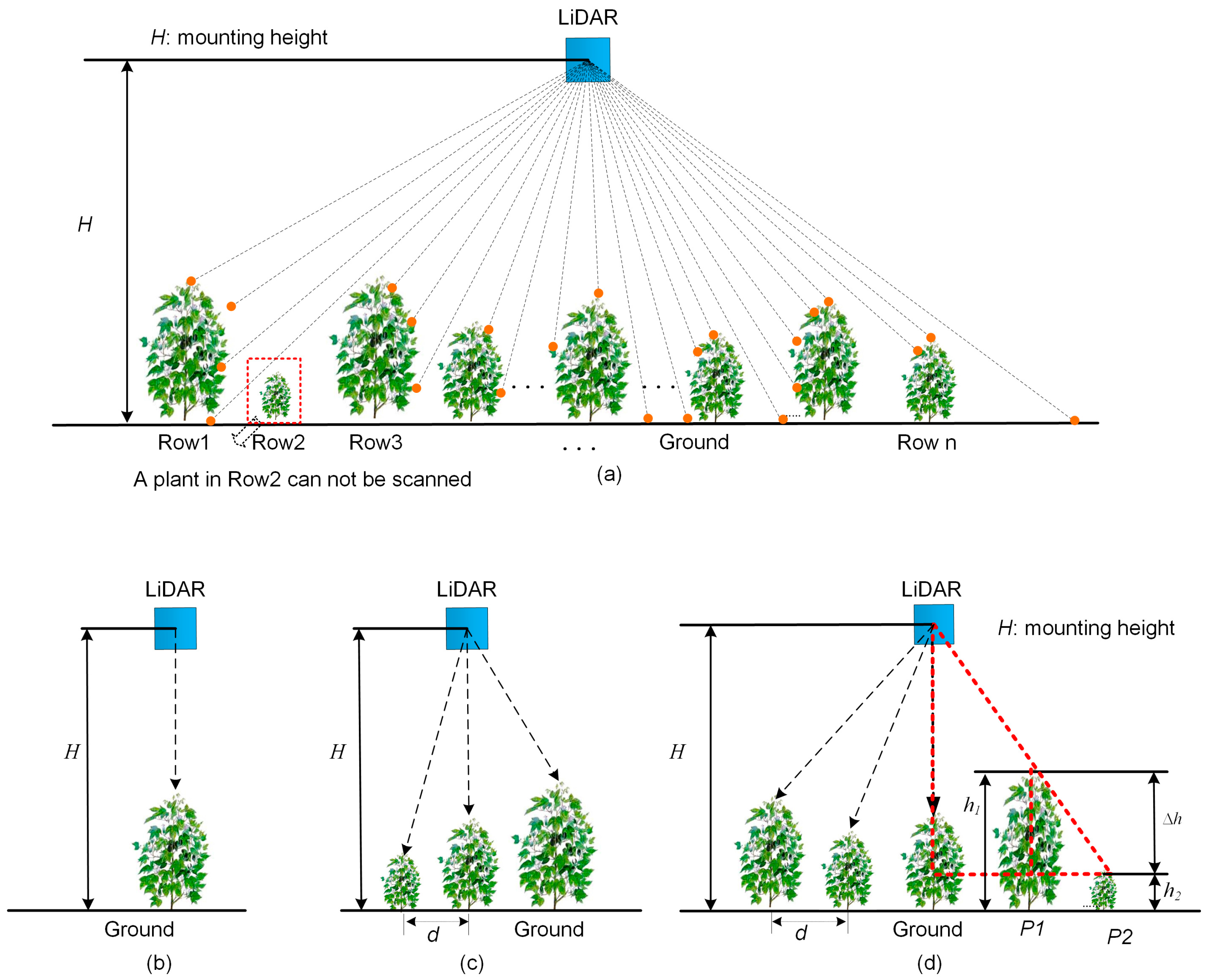
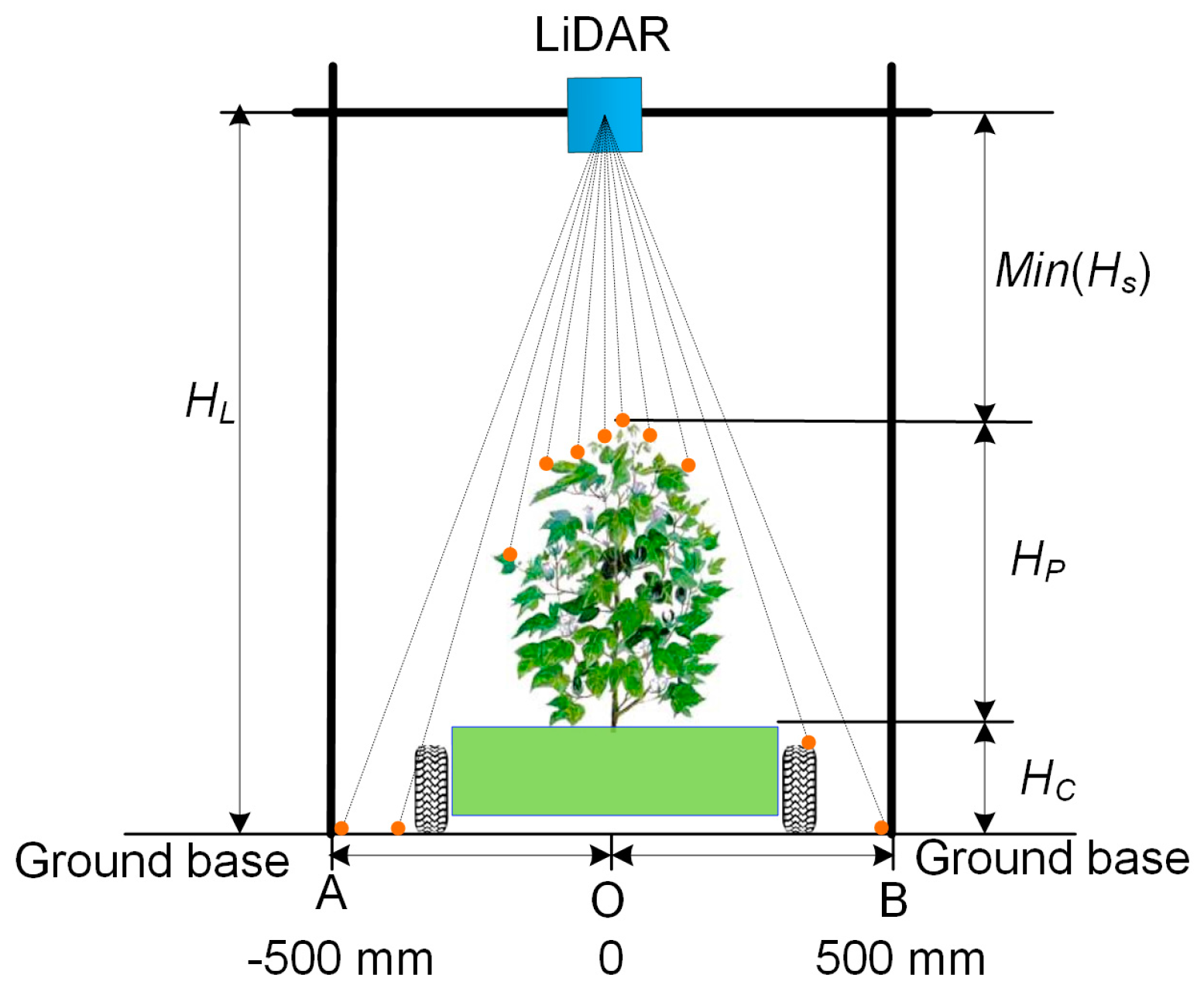
2.2.2. Mounting Height
2.2.3. Moving Speed of the Sensor Unit
2.3. Experimental Setup
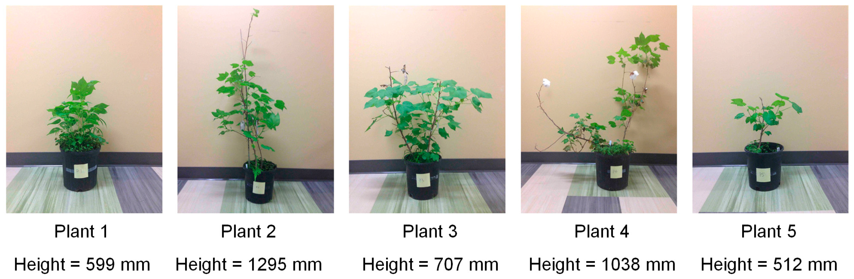
2.3.1. Lab Experiment Setup
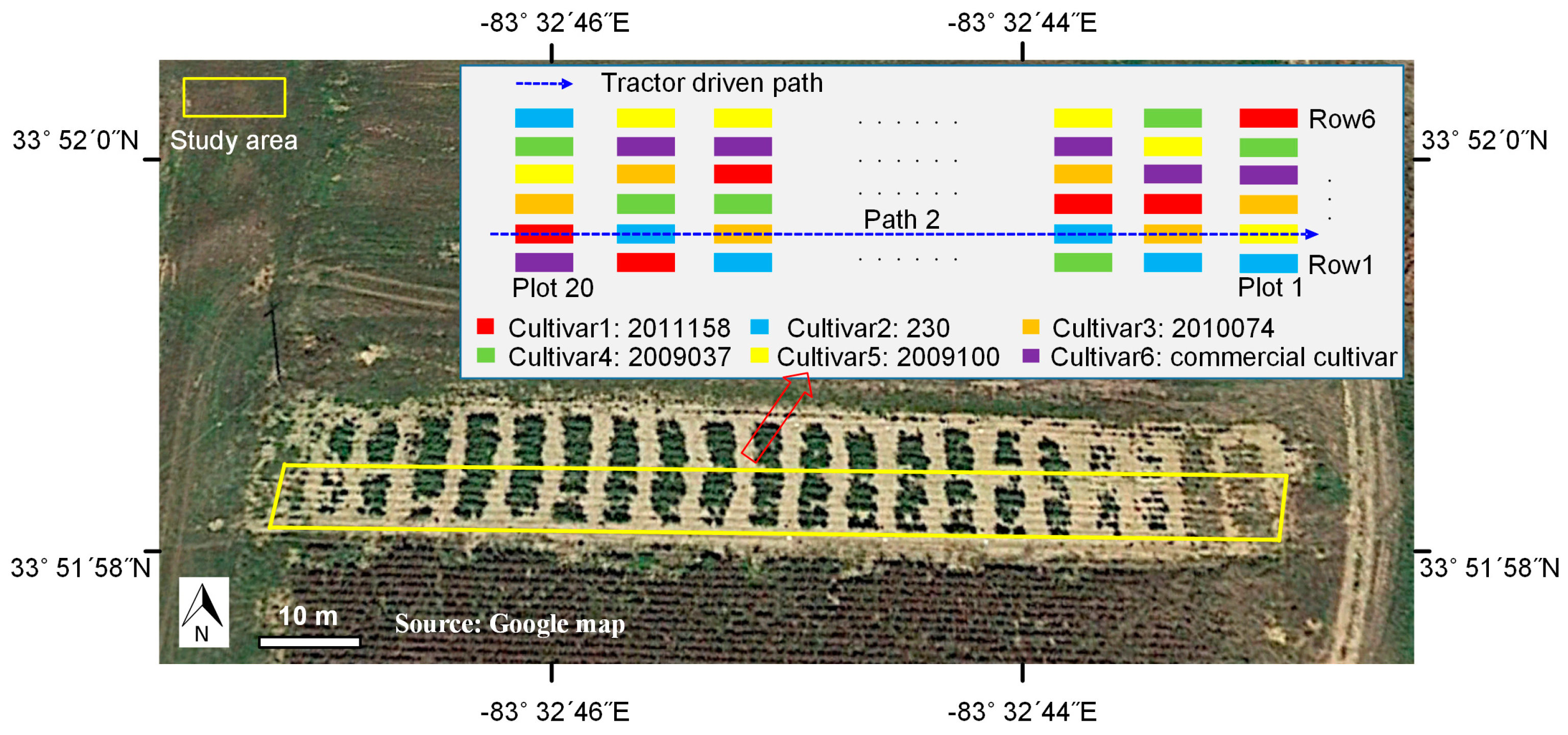
2.3.2. Field Experiment Setup
2.4. Data Processing Algorithm and Performance Evalutaion
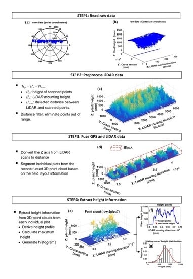
- Step 1
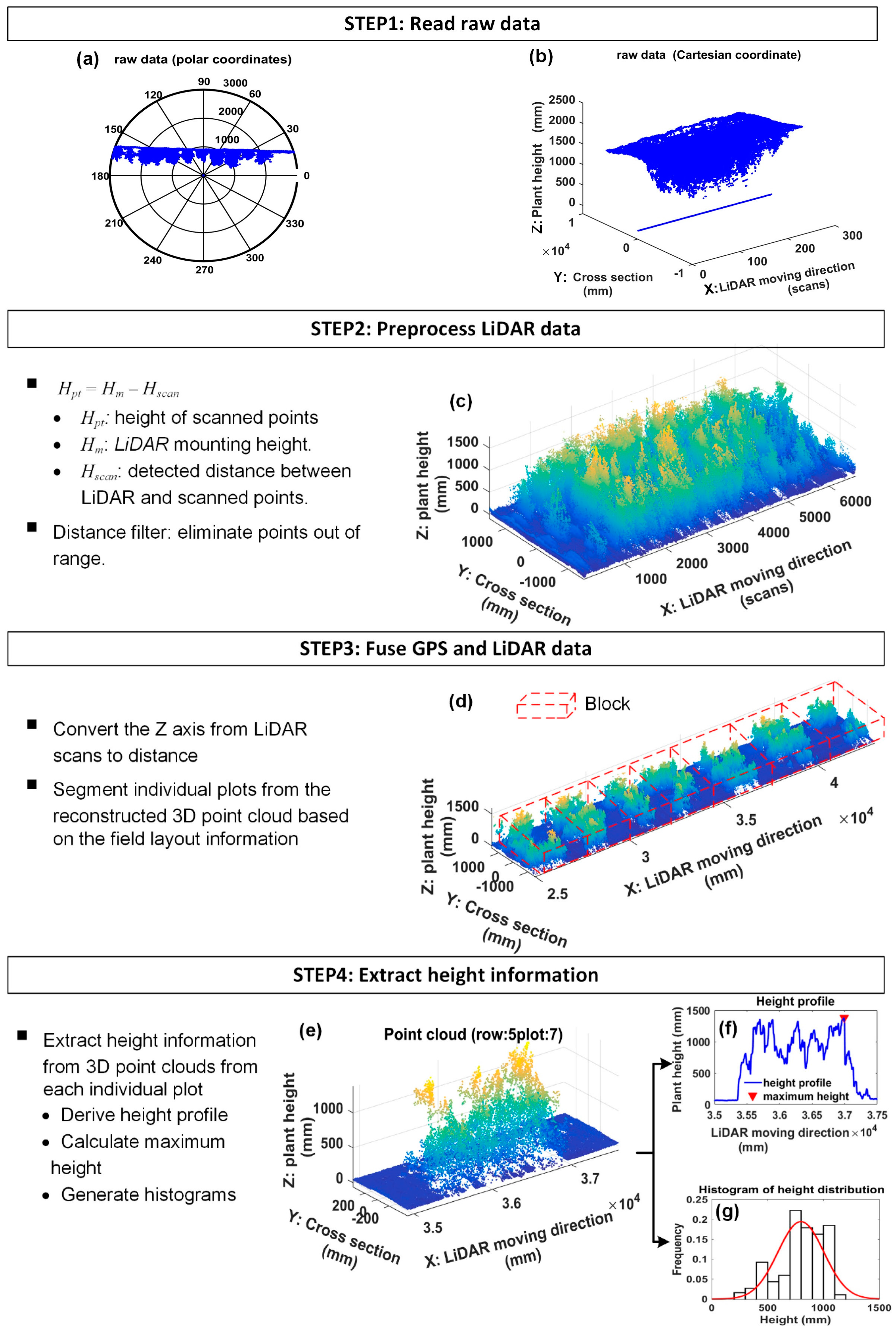
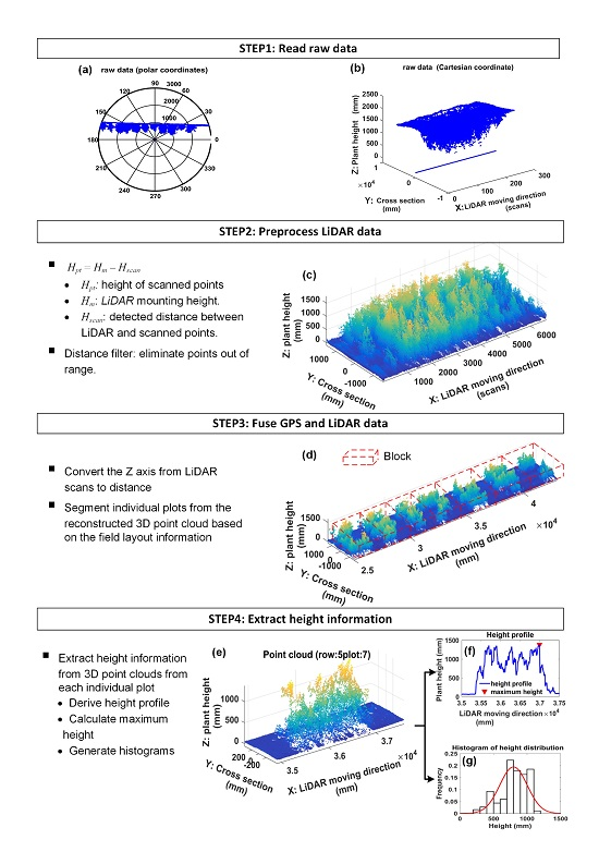
- Read raw dataThe LiDAR scanned frames including timestamps, and GPS tags were retrieved from test files by a program developed in MATLAB 2016a. The raw LiDAR data is shown in Figure 10a,b.
- Step 2
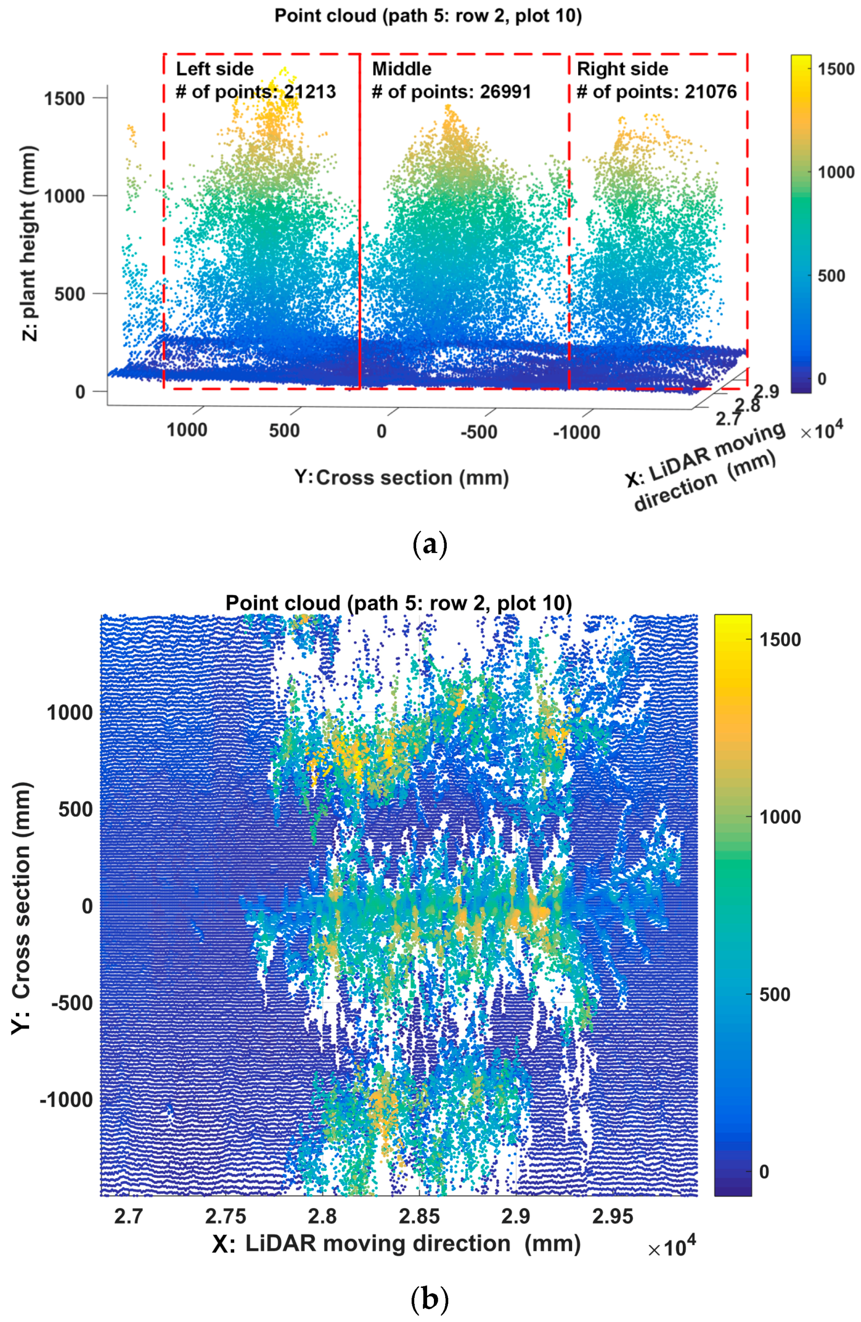
- Preprocess the point cloud of LiDARThe raw data along the Y axis was processed using Equation (10):where Hm is the LiDAR mounting height, Hscan is the detected distance between each scanned point along the Y axis and the LiDAR, and Hpt is the real height value of each scanned point. Distance filters were then used to eliminate out-of-range data along the Y and Z axis. Along the Y-axis direction, the distance filter threshold was determined by the rows scanned by the LiDAR. For example, if three rows were scanned at a time, the threshold would be 1372 mm which is equal to 1.5 times the length of interspace between two rows. Along the Z-axis direction, the threshold is set to be the mounting height of the LiDAR; points below the LiDAR were kept. An example of reconstructed 3D point clouds is shown in Figure 10c. The Y axis was the direction of cross section, the Z axis depicted the plant height, and the X-axis denoted the tractor’s direction of movement. The Y-axis and Z-axis indicate lengths in millimeters, while the X-axis indicates the number of scanned frames since GPS data was not merged.
- Step 3
- Fuse GPS data with LiDAR dataGPS data was used to make the conversion of the unit of the X-axis from the frame number to distance. Let PGPS be the set of collected GPS data, and FLiDAR be the set of the scanned frames of LiDAR (Equation (11)). The number of GPS points was N, and the number of LiDAR frames is M. The GPS data and LiDAR data were synchronized using timestamp.The distance between two adjacent GPS points denoted by ΔPGPS was computed by Equation (12). fLiDAR and fGPS were the data acquisition frequency of LiDAR and GPS, respectively. In this study, the data acquisition frequency of GPS was fGPS = 5 Hz, and LiDAR scanning frequency was fLiDAR = 50 Hz. Therefore, there were 10 scanned frames, each containing 381 points (The aperture angle was 190° with angular resolution 0.5°), between every two adjacent GPS points (Equation (13)). Assume that the tractor was moving at a constant speed during the interval (200 ms) of two adjacent GPS points. The distance of the two adjacent frames within two adjacent GPS points was computed using Equation (14). Therefore, the position of each LiDAR scanned frame was able to be obtained using Equation (15). Doffset was the offset between LiDAR and GPS. In this study, Doffset was fixed during data collection in the field, and the measured point at 0° scanning angle was used to depict the frame position. Figure 10d showed the reconstructed 3D model with X-axis indicated by millimeter units. The point cloud of individual plot was retrieved from the 3D model based on the field layout information (Figure 9). First, the 3D model was segmented into 20 blocks along the tractor moving direction according to the premeasured start and end points of each row and the length of the plot, and then plots within each block were segmented based on the interspace between two rows.
- Step 4
- Extract height traitA canopy height profile (CHP) of one plot (Figure 10e) would be derived by calculating the maximum height of each frame. Based on CHP, the maximum height and histograms of canopy height were extracted (Figure 10f,g). A threshold of 200 mm was set for the histogram to segment the plants from the ground.
3. Results
3.1. Results of Lab Tests
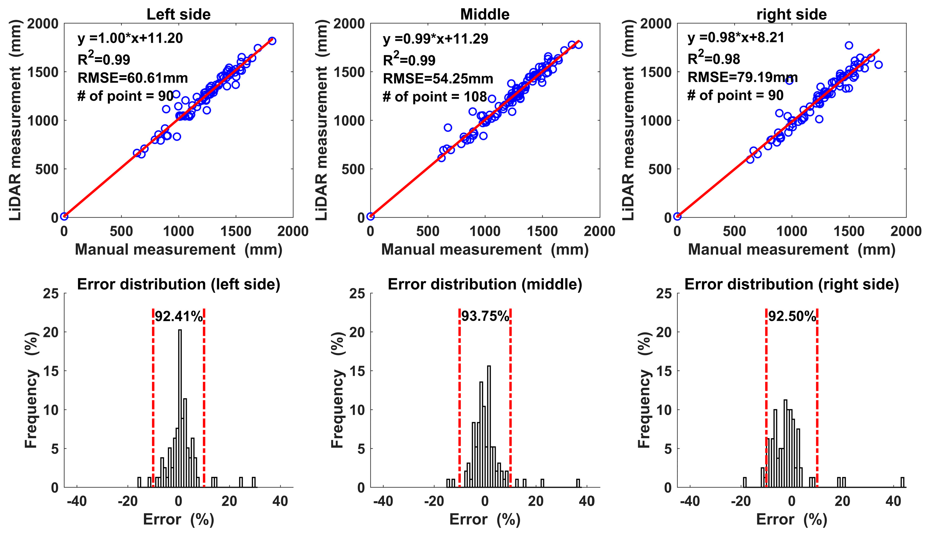
3.2. Results of Field Tests
4. Discussion
5. Conclusions
Acknowledgments
Author Contributions
Conflicts of Interest
References
- Garrido, M.; Paraforos, D.S.; Reiser, D.; Vázquez Arellano, M.; Griepentrog, H.W.; Valero, C. 3D maize plant reconstruction based on georeferenced overlapping lidar point clouds. Remote Sens. 2015, 7, 17077–17096. [Google Scholar] [CrossRef]
- Rosell-Polo, J.R.; Llorens, J.; Sanz, R.; Arnó, J.; Ribes-Dasi, M.; Masip, J.; Escolà, A.; Camp, F.; Solanelles, F.; Gràcia, F.; et al. Obtaining the three-dimensional structure of tree orchards from remote 2D terrestrial lidar scanning. Agric. For. Meteorol. 2009, 149, 1505–1515. [Google Scholar] [CrossRef]
- Großkinsky, D.K.; Pieruschka, R.; Svensgaard, J.; Rascher, U.; Christensen, S.; Schurr, U.; Roitsch, T. Phenotyping in the fields: Dissecting the genetics of quantitative traits and digital farming. New Phytol. 2015, 207, 950–952. [Google Scholar] [CrossRef] [PubMed]
- Goggin, F.L.; Lorence, A.; Topp, C.N. Applying high-throughput phenotyping to plant–insect interactions: Picturing more resistant crops. Curr. Opin. Insect Sci. 2015, 9, 69–76. [Google Scholar] [CrossRef]
- Cobb, J.N.; DeClerck, G.; Greenberg, A.; Clark, R.; McCouch, S. Next-generation phenotyping: Requirements and strategies for enhancing our understanding of genotype–phenotype relationships and its relevance to crop improvement. Theor. Appl. Genet. 2013, 126, 867–887. [Google Scholar] [CrossRef] [PubMed]
- Stamatiadis, S.; Tsadilas, C.; Schepers, J.S. Ground-based canopy sensing for detecting effects of water stress in cotton. Plant Soil 2010, 331, 277–287. [Google Scholar] [CrossRef]
- White, J.W.; Andrade-Sanchez, P.; Gore, M.A.; Bronson, K.F.; Coffelt, T.A.; Conley, M.M.; Feldmann, K.A.; French, A.N.; Heun, J.T.; Hunsaker, D.J.; et al. Review: Field-based phenomics for plant genetics research. Field Crop. Res. 2012, 133, 101–112. [Google Scholar] [CrossRef]
- Lipka, A.E.; Kandianis, C.B.; Hudson, M.E.; Yu, J.; Drnevich, J.; Bradbury, P.J.; Gore, M.A. From association to prediction: Statistical methods for the dissection and selection of complex traits in plants. Curr. Opin. Plant Biol. 2015, 24, 110–118. [Google Scholar] [CrossRef] [PubMed]
- Sharma, B.; Ritchie, G.L. High-throughput phenotyping of cotton in multiple irrigation environments. Crop Sci. 2015, 55, 958–969. [Google Scholar] [CrossRef]
- Granier, C.; Vile, D. Phenotyping and beyond: Modelling the relationships between traits. Curr. Opin. Plant Biol. 2014, 18, 96–102. [Google Scholar] [CrossRef] [PubMed]
- Ghanem, M.E.; Marrou, H.; Sinclair, T.R. Physiological phenotyping of plants for crop improvement. Trends Plant Sci. 2015, 20, 139–144. [Google Scholar] [CrossRef] [PubMed]
- Barker, J.; Zhang, N.; Sharon, J.; Steeves, R.; Wang, X.; Wei, Y.; Poland, J. Development of a field-based high-throughput mobile phenotyping platform. Comput. Electron. Agric. 2016, 122, 74–85. [Google Scholar] [CrossRef]
- Palanichamy, D.; Cobb, J.N. Agronomic field trait phenomics. In Phenomics; Springer: Berlin, Germany, 2015; pp. 83–99. [Google Scholar]
- Pratap, A.; Tomar, R.; Kumar, J.; Pandey, V.R.; Mehandi, S.; Katiyar, P.K. High-throughput plant phenotyping platforms. In Phenomics in Crop Plants: Trends, Options and Limitations; Springer: Berlin, Germany, 2015; pp. 285–296. [Google Scholar]
- Hofle, B. Radiometric correction of terrestrial lidar point cloud data for individual maize plant detection. IEEE Geosci. Remote Sens. Lett. 2014, 11, 94–98. [Google Scholar] [CrossRef]
- Zhang, L.; Grift, T.E. A LiDAR-based crop height measurement system for Miscanthus Giganteus. Comput. Electron. Agric. 2012, 85, 70–76. [Google Scholar] [CrossRef]
- Tilly, N.; Hoffmeister, D.; Cao, Q.; Huang, S.; Lenz-Wiedemann, V.; Miao, Y.; Bareth, G. Multitemporal crop surface models: Accurate plant height measurement and biomass estimation with terrestrial laser scanning in paddy rice. J. Appl. Remote Sens. 2014, 8. [Google Scholar] [CrossRef]
- Sritarapipat, T.; Rakwatin, P.; Kasetkasem, T. Automatic rice crop height measurement using a field server and digital image processing. Sensors 2014, 14, 900–926. [Google Scholar] [CrossRef] [PubMed]
- Siebert, J.D.; Stewart, A.M. Influence of plant density on cotton response to mepiquat chloride application. Agron. J. 2006, 98, 1634–1639. [Google Scholar] [CrossRef]
- Baloch, M.; Khan, N.; Rajput, M.; Jatoi, W.; Gul, G.; Rind, I.; Veesar, N. Yield related morphological measures of short duration cotton genotypes. J. Anim. Plant Sci. 2014, 24, 1198–1211. [Google Scholar]
- Andrade-Sanchez, P.; Gore, M.A.; Heun, J.T.; Thorp, K.R.; Carmo-Silva, A.E.; French, A.N.; Salvucci, M.E.; White, J.W. Development and evaluation of a field-based high-throughput phenotyping platform. Funct. Plant Biol. 2013, 41, 68–79. [Google Scholar] [CrossRef]
- Carlone, L.; Dong, J.; Fenu, S.; Rains, G.; Dellaert, F. Towards 4D crop analysis in precision agriculture: Estimating plant height and crown radius over time via expectation-maximization. In Proceedings of the ICRA Workshop on Robotics in Agriculture, Seattle, WA, USA, 30 May 2015. [Google Scholar]
- Furukawa, Y.; Ponce, J. Accurate, dense, and robust multiview stereopsis. IEEE Trans. Pattern Anal. Mach. Intell. 2010, 32, 1362–1376. [Google Scholar] [CrossRef] [PubMed]
- Kaess, M.; Johannsson, H.; Roberts, R.; Ila, V.; Leonard, J.J.; Dellaert, F. iSAM2: Incremental smoothing and mapping using the bayes tree. Int. J. Robot. Res. 2011, 31, 216–235. [Google Scholar] [CrossRef]
- Busemeyer, L.; Mentrup, D.; Möller, K.; Wunder, E.; Alheit, K.; Hahn, V.; Maurer, H.; Reif, J.; Würschum, T.; Müller, J.; et al. Breedvision—A multi-sensor platform for non-destructive field-based phenotyping in plant breeding. Sensors 2013, 13. [Google Scholar] [CrossRef] [PubMed]
- Lin, Y. LiDAR: An important tool for next-generation phenotyping technology of high potential for plant phenomics? Comput. Electron. Agric. 2015, 119, 61–73. [Google Scholar] [CrossRef]
- Leeuwen, M.V.; Nieuwenhuis, M. Retrieval of forest structural parameters using LiDAR remote sensing. Eur. J. For. Res. 2010, 129, 749–770. [Google Scholar] [CrossRef]
- Zhao, K.; Popescu, S. LiDAR-based mapping of leaf area index and its use for validating globcarbon satellite lai product in a temperate forest of the southern USA. Remote Sens. Environ. 2009, 113, 1628–1645. [Google Scholar] [CrossRef]
- Murgoitio, J.; Shrestha, R.; Glenn, N.; Spaete, L. Airborne LiDAR and terrestrial laser scanning derived vegetation obstruction factors for visibility models. Trans. GIS 2014, 18, 147–160. [Google Scholar] [CrossRef]
- Llorens, J.; Gil, E.; Llop, J. Ultrasonic and LiDAR sensors for electronic canopy characterization in vineyards: Advances to improve pesticide application methods. Sensors 2011, 11, 2177–2194. [Google Scholar] [CrossRef] [PubMed]
- Rosell Polo, J.R.; Sanz, R.; Llorens, J.; Arnó, J.; Escolà, A.; Ribes-Dasi, M.; Masip, J.; Camp, F.; Gràcia, F.; Solanelles, F.; et al. A tractor-mounted scanning LiDAR for the non-destructive measurement of vegetative volume and surface area of tree-row plantations: A comparison with conventional destructive measurements. Biosyst. Eng. 2009, 102, 128–134. [Google Scholar] [CrossRef]
- Cheein, F.A.A.; Guivant, J.; Sanz, R.; Escolà, A.; Yandún, F.; Torres-Torriti, M.; Rosell-Polo, J.R. Real-time approaches for characterization of fully and partially scanned canopies in groves. Comput. Electron. Agric. 2015, 118, 361–371. [Google Scholar] [CrossRef]
- Pforte, F.; Selbeck, J.; Hensel, O. Comparison of two different measurement techniques for automated determination of plum tree canopy cover. Biosyst. Eng. 2012, 113, 325–333. [Google Scholar] [CrossRef]
- Sanz-Cortiella, R.; Llorens-Calveras, J.; Escolà, A.; Arnó-Satorra, J.; Ribes-Dasi, M.; Masip-Vilalta, J.; Camp, F.; Gràcia-Aguilá, F.; Solanelles-Batlle, F.; Planas-DeMartí, S.; et al. Innovative LiDAR 3D dynamic measurement system to estimate fruit-tree leaf area. Sensors 2011, 11. [Google Scholar] [CrossRef] [PubMed]
- Shi, Y.; Wang, N.; Taylor, R.K.; Raun, W.R. Improvement of a ground-LIDAR-based corn plant population and spacing measurement system. Comput. Electron. Agric. 2015, 112, 92–101. [Google Scholar] [CrossRef]
- Kjaer, K.H.; Ottosen, C.O. 3D laser triangulation for plant phenotyping in challenging environments. Sensors 2015, 15, 13533–13547. [Google Scholar] [CrossRef] [PubMed]
- Bhardwaj, A.; Sam, L.; Bhardwaj, A.; Martín-Torres, F.J. LiDAR remote sensing of the cryosphere: Present applications and future prospects. Remote Sens. Environ. 2016, 177, 125–143. [Google Scholar] [CrossRef]
- Mauney, J.R. Vegetative growth and development of fruiting sites. In Cotton Physiology: The Cotton Foundation Reference Book Series No 1.; The Cotton Foundation: Memphis, TN, USA, 1986; pp. 11–28. [Google Scholar]
- Andújar, D.; Rosell-Polo, J.; Sanz, R.; Rueda-Ayala, V.; Fernández-Quintanilla, C.; Ribeiro, A.; Dorado, J. A LiDAR-based system to assess poplar biomass. Gesunde Pflanz. 2016, 68, 155–162. [Google Scholar] [CrossRef]
- SICK, A. Operation Instructions LMS5XX Laser Measurement Sensors. Available online: https://www.Sick.Com/media/dox/4/14/514/operating_instructions_laser_measurement_sensors_of_the_lms5xx_product_family_en_im0037514.Pdf (accessed on 17 April 2017).
- Tilly, N.; Hoffmeister, D.; Cao, Q.; Lenz-Wiedemann, V.; Miao, Y.; Bareth, G. Transferability of models for estimating paddy rice biomass from spatial plant height data. Agriculture 2015, 5, 538–560. [Google Scholar] [CrossRef]
- Crommelinck, S.; Höfle, B. Simulating an autonomously operating low-cost static terrestrial LiDAR for multitemporal maize crop height measurements. Remote Sens. 2016, 8. [Google Scholar] [CrossRef]
- Steder, B.; Rusu, R.B.; Konolige, K.; Burgard, W. Point feature extraction on 3d range scans taking into account object boundaries. In Proceedings of the IEEE international conference on Robotics and Automation (ICRA), Shanghai, China, 9–13 May 2011. [Google Scholar]
- Luo, S.; Wang, C.; Pan, F.; Xi, X.; Li, G.; Nie, S.; Xia, S. Estimation of wetland vegetation height and leaf area index using airborne laser scanning data. Ecol. Indic. 2015, 48, 550–559. [Google Scholar] [CrossRef]


| Features | Performance | ||
|---|---|---|---|
| Operating range | 0~80 m | Systematic error | ±25 mm (1 m~10 m) |
| ±35 mm (10 m~20 m) | |||
| ±50 mm (20 m~30 m) | |||
| Aperture angle | 190° (−5°~185°) | Statistical error | 6 mm (1 m~10 m) |
| 8 mm (10 m~20 m) | |||
| 14 mm (20 m~30 m) | |||
| Scanning frequency | 25/35/50/75/100 Hz | Interface | Ethernet, RS-232,RS-422, USB, CAN |
| Angular resolution | 0.167/0.25/0.333/0.5/0.667/1° | Supply voltage | 24 V (22 W) |
| Wave length | Infrared (905 nm) | Temperature range | −30 °C to +50 °C |
| Features | Performance | ||
|---|---|---|---|
| Sampling frequency | 1, 5 and 10 Hz | Interface | RS-232, USB, CAN |
| RTK accuracy | 1 cm | Supply voltage | 9–16 V DC (600 mA) |
| Differential correction | SBAS (RTK) | Temperature range | −30 °C to +70 °C |
| NEMA output | GGA, GLL, GSA, GSV, RMC, VTG, ZDA | Memory | FLASH, 256 MB |
| Angular Resolution | Plant No. | Mean | |||||
|---|---|---|---|---|---|---|---|
| 1 | 2 | 3 | 4 | 5 | |||
| Manual Measurement (mm) | 599 | 1295 | 707 | 1038 | 512 | / | |
| 0.33° | Height (mm) | 598 | 1296 | 702 | 1033 | 508 | / |
| Error (%) | −0.14 | 0.09 | −0.68 | −0.47 | −0.84 | −0.41 | |
| Std 1 | 2.01 | 1.72 | 1.03 | 4.79 | 1.38 | 2.39 | |
| 0.5° | Height (mm) | 600 | 1292 | 702 | 1035 | 508 | / |
| Error (%) | 0.19 | −0.20 | −0.71 | −0.27 | −0.85 | −0.37 | |
| Std | 3.75 | 4.21 | 2.19 | 3.42 | 2.83 | 3.28 | |
| 1° | Height (mm) | 599 | 1292 | 702 | 1035 | 506 | / |
| Error (%) | −0.01 | −0.26 | −0.76 | −0.31 | −1.26 | −0.52 | |
| Std | 3.90 | 4.42 | 2.51 | 3.16 | 3.91 | 3.58 | |
| 3° | Height (mm) | 595 | 1289 | 698 | 1032 | 501 | / |
| Error (%) | −0.67 | −0.46 | −1.27 | −0.58 | −2.15 | −1.03 | |
| Std | 3.18 | 4.29 | 2.10 | 5.02 | 5.09 | 3.94 | |
| Overall | Left Side | Middle | Right Side | |
|---|---|---|---|---|
| Mean Error 1 (%) | −0.02 | 1.34 | 0.40 | −1.86 |
| Std Error 2 (%) | 6.84 | 6.27 | 6.23 | 7.69 |
© 2017 by the authors. Licensee MDPI, Basel, Switzerland. This article is an open access article distributed under the terms and conditions of the Creative Commons Attribution (CC BY) license (http://creativecommons.org/licenses/by/4.0/).
Share and Cite
Sun, S.; Li, C.; Paterson, A.H. In-Field High-Throughput Phenotyping of Cotton Plant Height Using LiDAR. Remote Sens. 2017, 9, 377. https://doi.org/10.3390/rs9040377
Sun S, Li C, Paterson AH. In-Field High-Throughput Phenotyping of Cotton Plant Height Using LiDAR. Remote Sensing. 2017; 9(4):377. https://doi.org/10.3390/rs9040377
Chicago/Turabian StyleSun, Shangpeng, Changying Li, and Andrew H. Paterson. 2017. "In-Field High-Throughput Phenotyping of Cotton Plant Height Using LiDAR" Remote Sensing 9, no. 4: 377. https://doi.org/10.3390/rs9040377
APA StyleSun, S., Li, C., & Paterson, A. H. (2017). In-Field High-Throughput Phenotyping of Cotton Plant Height Using LiDAR. Remote Sensing, 9(4), 377. https://doi.org/10.3390/rs9040377