
Sea Ice Concentration Estimation during Freeze-Up from SAR Imagery Using a Convolutional Neural Network


Abstract
:
1. Introduction
2. Background
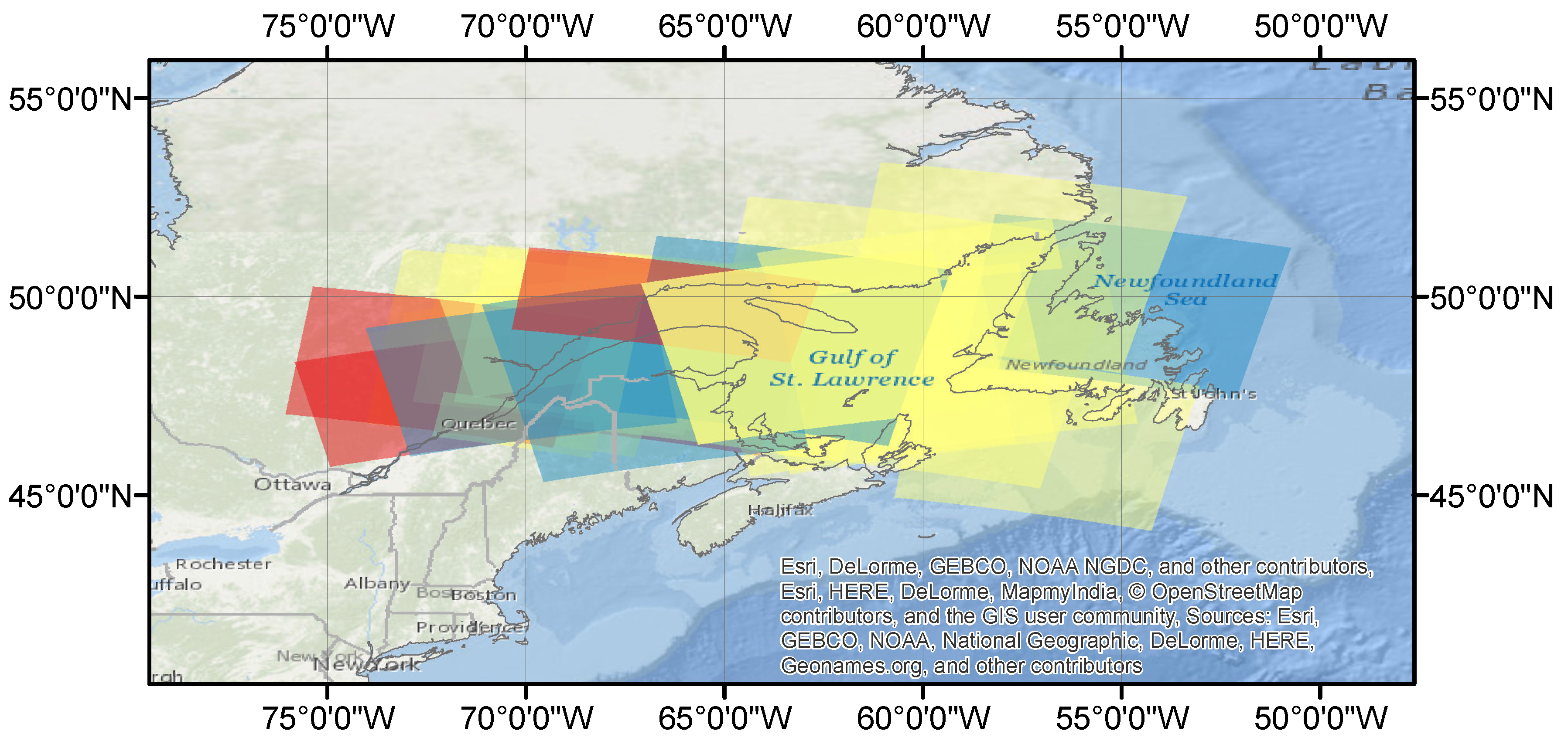
3. Data and Study Area
4. Methodology
4.1. Preprocessing of SAR Images
4.2. Overview and Structure of the CNN
4.3. Training and Testing
4.4. Implementation
5. An MLP for Ice Concentration Estimation
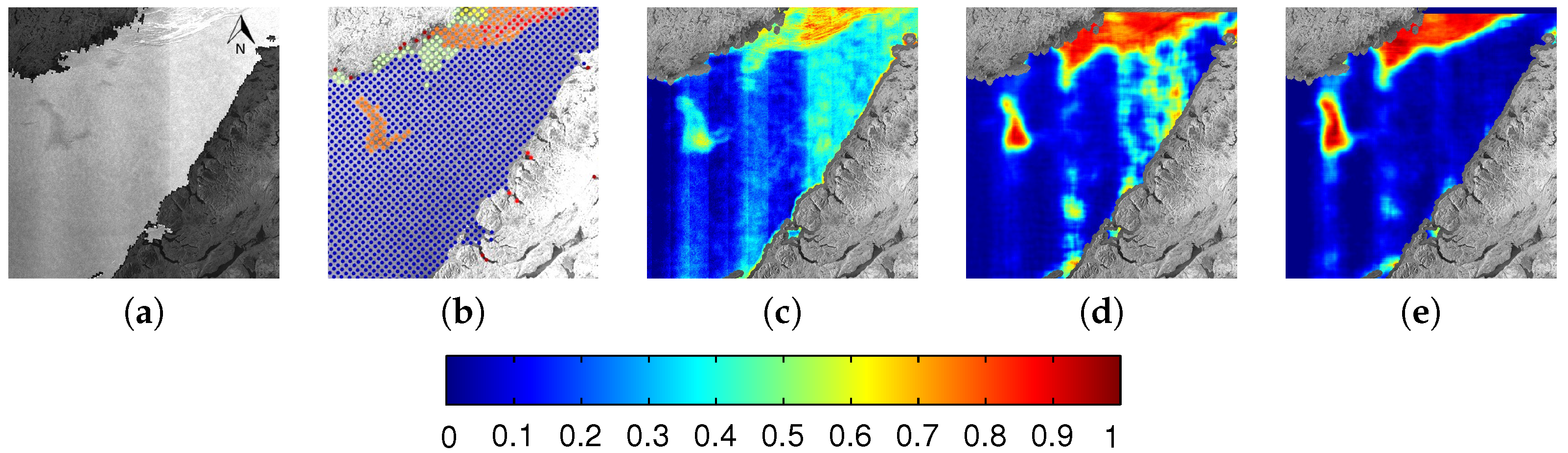
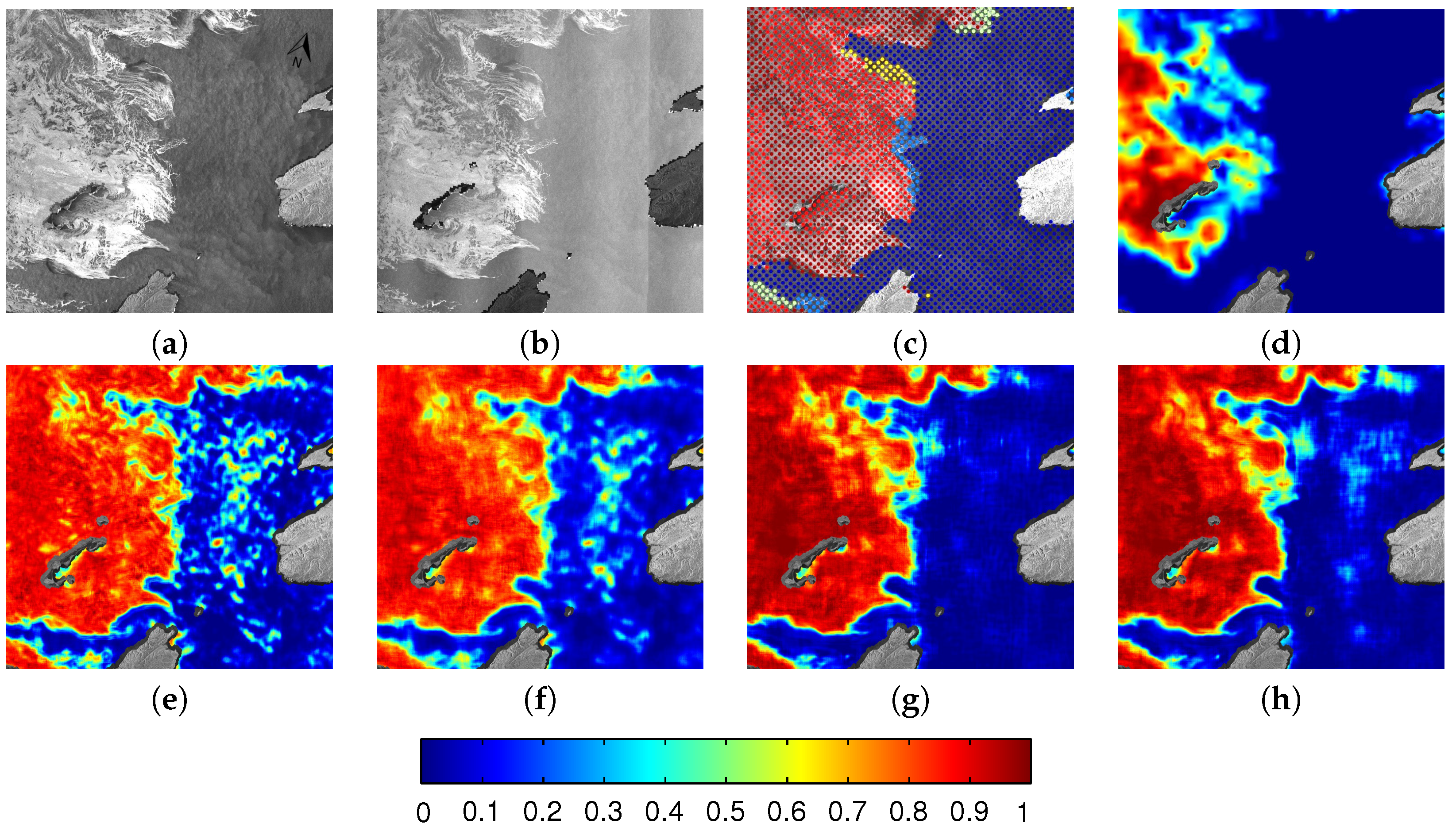
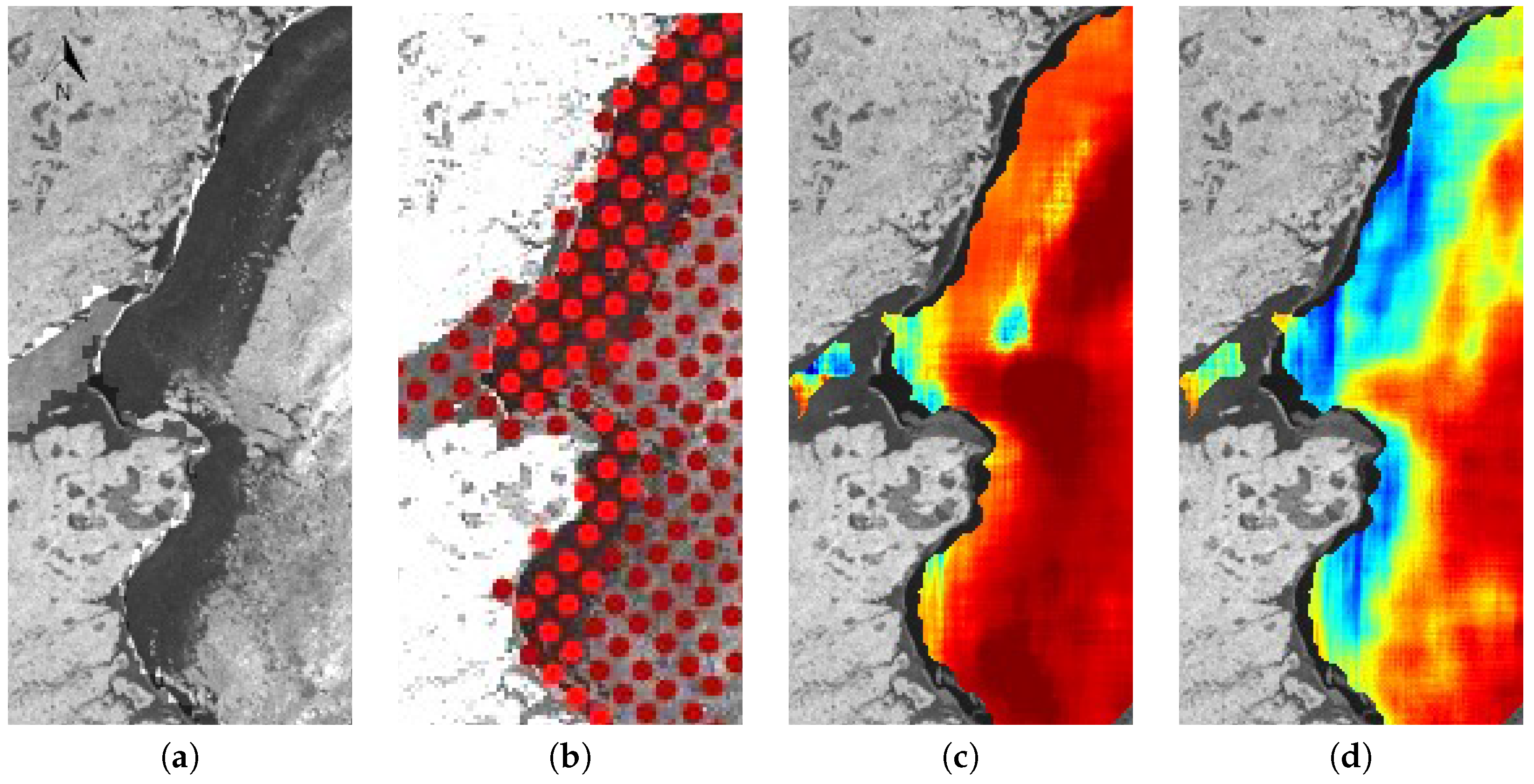
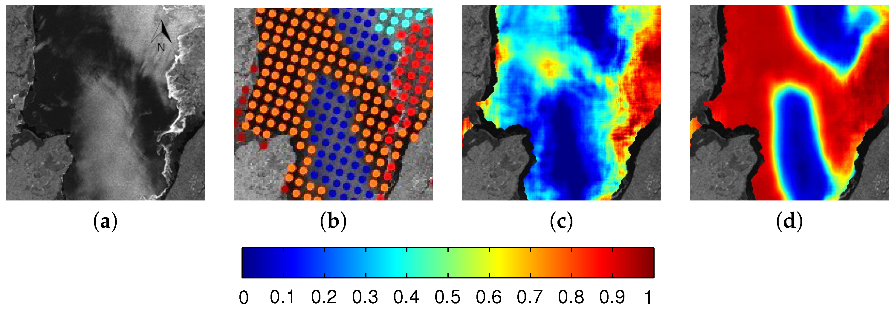
6. Results
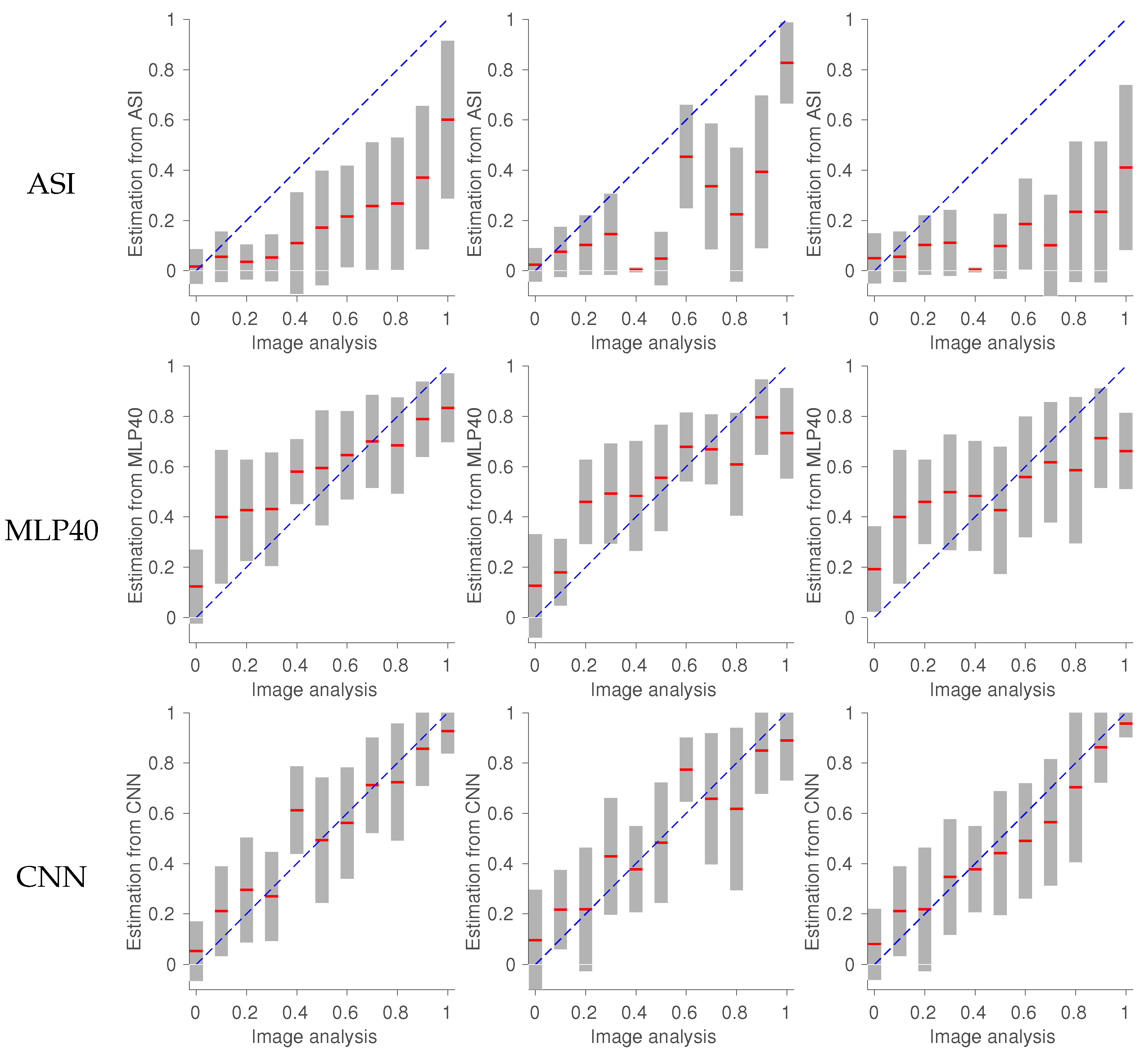
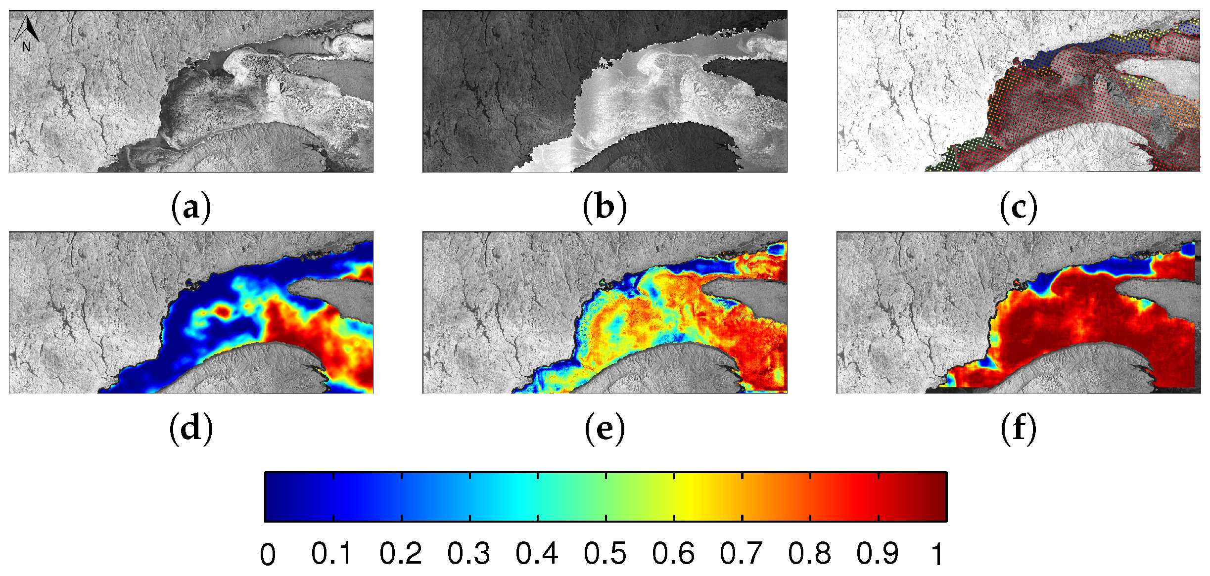
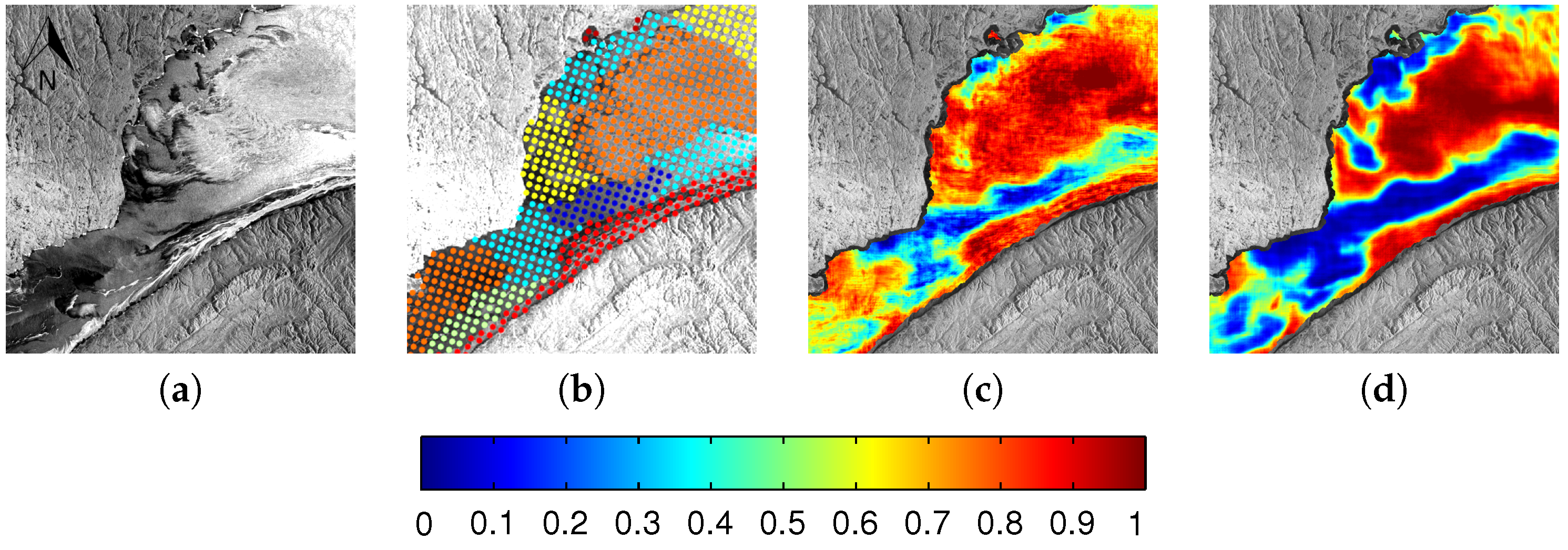
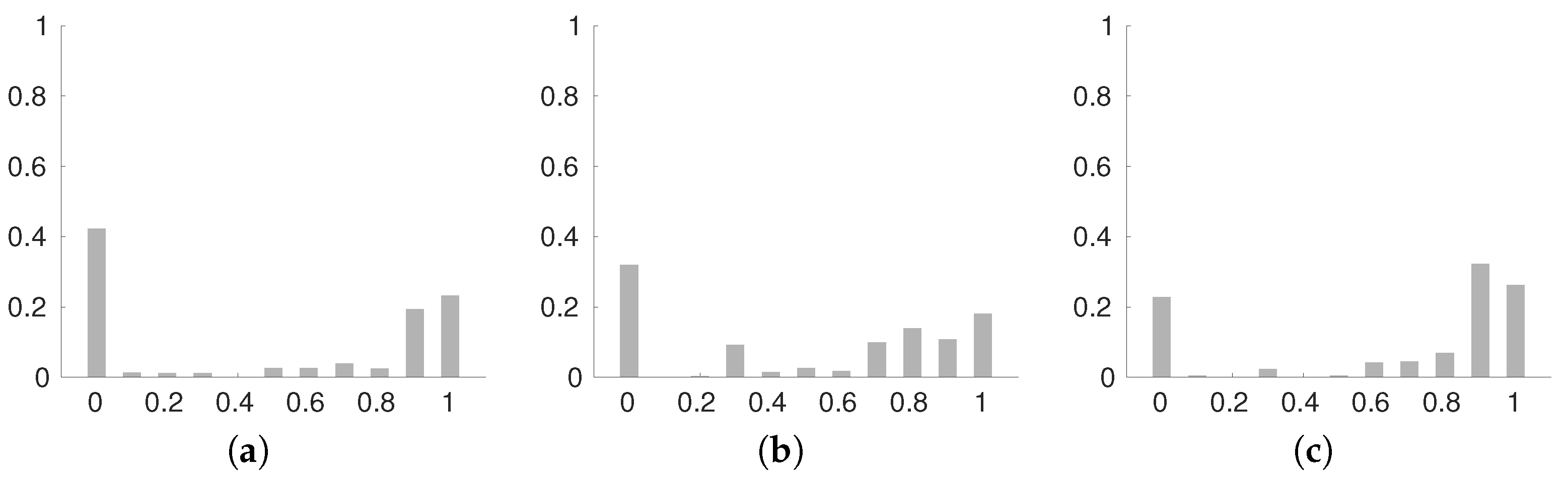
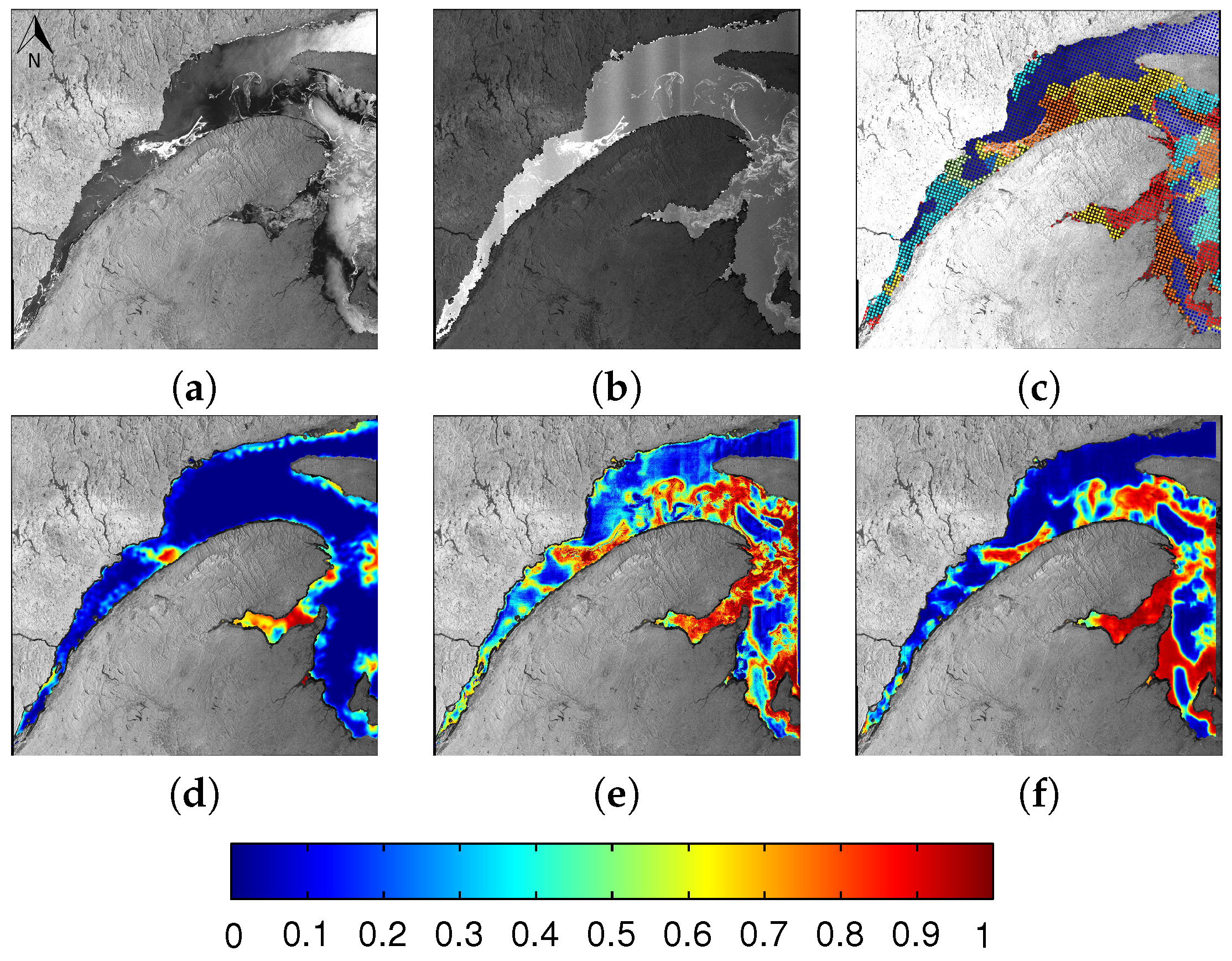
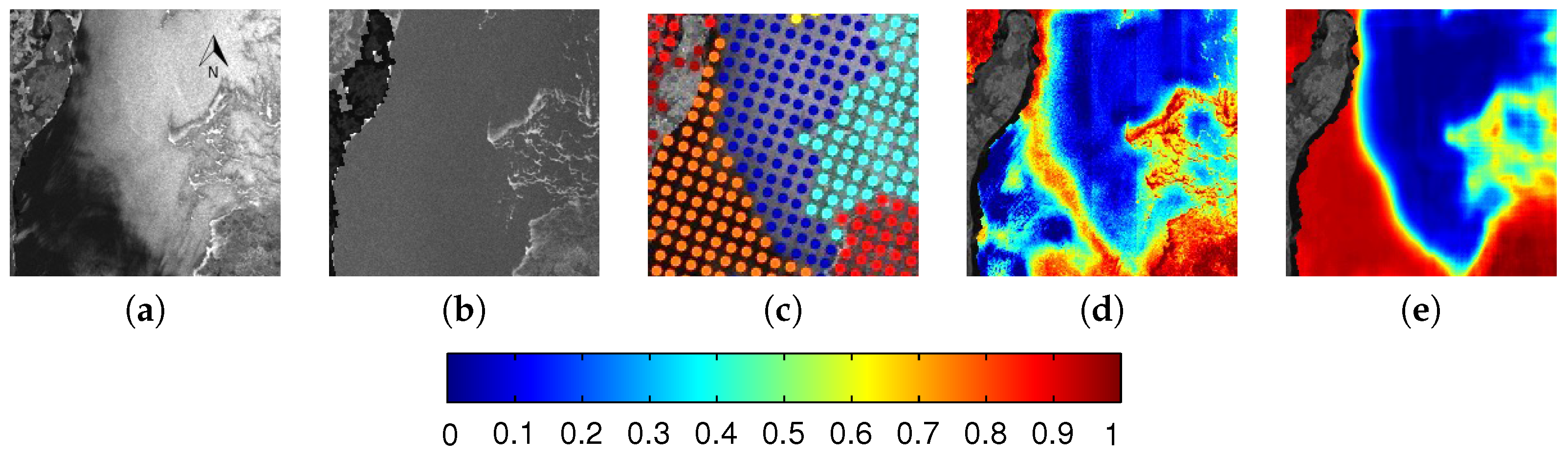
6.1. Evaluation
6.2. Comparison between MLP and CNN
6.3. Evaluation of CNN Architecture and Parameters
6.3.1. Patch Size
6.3.2. Use of Incidence Angle Data
6.3.3. Network Depth
7. Discussion
8. Conclusions
Acknowledgments
Author Contributions
Conflicts of Interest
References
- Carrieres, T.; Greenan, B.; Prinsenberg, S.; Peterson, I. Comparison of Canadian daily ice charts with surface observations off Newfoundland, winter 1992. Atmos. Ocean 1996, 34, 207–226. [Google Scholar] [CrossRef]
- Arkett, M.; Braithwaite, L.; Pestieau, P.; Carrieres, T.; Pogson, L.; Fabi, C.; Geldsetzer, T. Preparation by the Canadian Ice Service for the operational use of the RADARSAT Constellation Mission in their ice and oil spill monitoring programs. Can. J. Remote Sens. 2015, 41, 380–389. [Google Scholar] [CrossRef]
- Karvonen, J. Baltic sea ice concentration estimation based on C-band HH-polarized SAR data. Sel. Top. Appl. Earth Obs. Remote Sens. 2012, 5, 1874–1884. [Google Scholar] [CrossRef]
- Karvonen, J. Baltic sea ice concentration estimation based on C-band dual-polarized SAR data. IEEE Trans. Geosci. Remote Sens. 2014, 52, 5558–5566. [Google Scholar] [CrossRef]
- Clausi, D.A. Comparison and fusion of co-occurrence, Gabor, and MRF texture features for classification of SAR sea ice imagery. Atmos. Ocean 2001, 39, 183–194. [Google Scholar] [CrossRef]
- Deng, H.; Clausi, D.A. Unsupervised segmentation of synthetic aperture radar sea ice imagery using a novel Markov random field model. IEEE Trans. Geosci. Remote Sens. 2005, 43, 528–538. [Google Scholar] [CrossRef]
- Leigh, S.; Wang, Z.; Clausi, D.A. Automated ice-water classification using dual polarization SAR satellite imagery. IEEE Trans. Geosci. Remote Sens. 2014, 52, 5529–5539. [Google Scholar] [CrossRef]
- Zakhvatkina, N.Y.; Alexandrov, V.Y.; Johannessen, O.M.; Sandven, S.; Frolov, I.Y. Classification of Sea Ice Types in ENVISAT Synthetic Aperture Radar Images. IEEE Trans. Geosci. Remote Sens. 2013, 51, 2587–2600. [Google Scholar] [CrossRef]
- Liu, J.; Scott, K.; Gawish, A.; Fieguth, P. Automatic detection of the ice edge in SAR imagery using curvelet transform and active contour. Remote Sens. 2016, 8. [Google Scholar] [CrossRef]
- Pogson, L.; Geldsetzer, T.; Buehner, M.; Carrieres, T.; Ross, M.; Scott, K. A collection of empirically-derived characteristic values from SAR across a year of sea ice environments for use in data assimilation. Mon. Weather Rev. 2016, in press. [Google Scholar]
- Buehner, M.; Caya, A.; Pogson, L.; Carrieres, T.; Pestieau, P. A new Environment Canada regional ice analysis system. Atmos. Ocean 2013, 51, 18–34. [Google Scholar] [CrossRef]
- Drusch, M. Sea ice concentration analyses for the Baltic Sea and their impact on numerical weather prediction. J. Appl. Meteorol. Climatol. 2006, 45, 982–994. [Google Scholar] [CrossRef]
- LeCun, Y.; Bengio, J.; Hinton, G. Deep Learning. Nature 2015, 521, 436–444. [Google Scholar] [CrossRef] [PubMed]
- Wang, L.; Scott, K.A.; Xu, L.; Clausi, D.A. Sea Ice Concentration Estimation During Melt From Dual-Pol SAR Scenes Using Deep Convolutional Neural Networks: A Case Study. IEEE Trans. Geosci. Remote Sens. 2016, 54, 4524–4533. [Google Scholar] [CrossRef]
- Geldsetzer, T.; Yackel, J. Sea ice type and open water discrimination using dual co-polarized C-band SAR. Can. J. Remote Sens. 2009, 35, 73–84. [Google Scholar] [CrossRef]
- Ivanova, N.; Tonboe, R.; Pedersen, L.T. SICCI Product Validation and Algorithm Selection Report (PVASR)—Sea Ice Concentration; Technical Report; European Space Agency: Paris, France, 2013. [Google Scholar]
- Dumbill, E. Strata 2012: Making Data Work; O’Reilly: Santa Clara, CA, USA, 2012. [Google Scholar]
- Najafabadi, M.M.; Villanustre, F.; Khoshgoftaar, T.M.; Seliya, N.; Wald, R.; Muharemagic, E. Deep learning applications and challenges in big data analytics. J. Big Data 2015, 2. [Google Scholar] [CrossRef]
- National Research Council. Frontiers in Massive Data Analysis; The National Academies Press: Washington, DC, USA, 2013. [Google Scholar]
- Domingos, P. A Few Useful Things to Know About Machine Learning. Commun. ACM 2012, 55, 78–87. [Google Scholar] [CrossRef]
- Bengio, Y.; Courville, A.; Vincent, P. Representation learning: A review and new perspectives. IEEE Trans. Pattern Anal. Mach. Intell. 2013, 35, 1798–1828. [Google Scholar] [CrossRef] [PubMed]
- Hinton, G.E. Learning multiple layers of representation. Trends Cogn. Sci. 2007, 11, 428–434. [Google Scholar] [CrossRef] [PubMed]
- Bengio, Y. Learning deep architectures for AI. Found. Trends Mach. Learn. 2009, 2, 1–127. [Google Scholar] [CrossRef]
- Lee, H.; Grosse, R.; Ranganath, R.; Ng, A.Y. Convolutional deep belief networks for scalable unsupervised learning of hierarchical representations. In Proceedings of the 26th Annual International Conference on Machine Learning, Montreal, QC, Canada, 14–18 June 2009; pp. 609–616. [Google Scholar]
- Ciresan, D.C.; Meier, U. Flexible, high performance convolutional neural networks for image classification. In Proceedings of the Twenty-Second International Joint Conference On Artificial Intelligence, Barcelona, Spain, 16–22 July 2011; pp. 1237–1242. [Google Scholar]
- Krizhevsky, A.; Sutskever, I.; Hinton, G.E. ImageNet classification with deep convolutional neural networks. In Proceedings of the 25th International Conference on Neural Information Processing Systems, Lake Tahoe, NV, USA, 3–6 December 2012; pp. 1097–1105. [Google Scholar]
- Karpathy, A.; Toderici, G.; Shetty, S.; Leung, T.; Sukthankar, R.; Fei-Fei, L. Large-scale video classification with convolutional neural networks. In Proceedings of the 2014 IEEE Conference on Computer Vision and Pattern Recognition, Columbus, OH, USA, 23–28 June 2014; pp. 1725–1732. [Google Scholar]
- Mnih, V.; Hinton, G.E. Learning to detect roads in high-resolution aerial images. In Computer Vision-ECCV 2010; Springer: Berlin/Heidelberg, Germany, 2010; pp. 210–223. [Google Scholar]
- Chen, X.; Xiang, S.; Liu, C.L.; Pan, C.H. Vehicle Detection in Satellite Images by Hybrid Deep Convolutional Neural Networks. IEEE Geosci. Remote Sens. Lett. 2014, 11, 1797–1801. [Google Scholar] [CrossRef]
- Maggiori, E.; Tarabalka, Y.; Charpiat, G.; Alliez, P. Fully convolutional neural networks for remote sensing image classification. In Proceedings of the 2016 IEEE Geoscience and Remote Sensing Symposium, Beijing, China, 10–15 July 2016. [Google Scholar]
- Spreen, G.; Kaleschke, L.; Heygster, G. Sea ice remote sensing using AMSR-E 89-GHz channels. J. Geophys. Res. 2008, 113. [Google Scholar] [CrossRef]
- Agnew, T.; Howell, S. The use of operational ice charts for evaluating passive microwave ice concentration data. Atmos. Ocean 2003, 41, 317–331. [Google Scholar] [CrossRef]
- Karvonen, J.; Vainio, J.; Marnela, M.; Eriksson, P.; Niskanen, T. A comparison between high-resolution EO-based and ice analyst-assigned sea ice concentrations. J. Sel. Top. Appl. Earth Obs. Remote Sens. 2015, 8, 1799–1807. [Google Scholar] [CrossRef]
- Fequest, D. MANICE: Manual of Standard Procedures for Observing and Reporting Ice Conditions; Environment Canada: Ottawa, ON, Canada, 2002. [Google Scholar]
- Slade, B. RADARSAT-2 Product Description; MacDonald, Dettwiler and Associates Ltd.: Richmond, BC, Canada, 2009. [Google Scholar]
- Moen, A.; Doulgeris, P.; Anfinsen, S.; Renner, A.; Hughes, N.; Gerland, S.; Eltoft, T. Comparison of feature based segmentation of full polarimetric SAR satellite sea ice images with manually drawn ice charts. Cryosphere 2013, 7, 1693–1705. [Google Scholar] [CrossRef]
- De Andrade, A. Best Practices for Convolutional Neural Networks Applied to Object Recognition in Images; Technical Report; Department of Computer Science, University of Toronto: Toronto, ON, USA, 2014. [Google Scholar]
- LeCun, Y.; Bottou, L.; Bengio, Y.; Haffner, P. Gradient-based learning applied to document recognition. Proc. IEEE 1998, 86, 2278–2324. [Google Scholar] [CrossRef]
- LeCun, Y.; Huang, F.J.; Bottou, L. Learning methods for generic object recognition with invariance to pose and lighting. In Proceedings of the 2004 IEEE Computer Society Conference on Computer Vision and Pattern Recognition, Washington, DC, USA, 27 June–2 July 2004. [Google Scholar]
- LeCun, Y.; Kavukcuoglu, K.; Farabet, C. Convolutional networks and applications in vision. Proceedings of 2010 IEEE International Symposium on Circuits and Systems (ISCAS), Paris, France, 30 May–2 June 2010; pp. 253–256. [Google Scholar]
- Chen, L.C.; Papandreou, G.; Kokkinos, I.; Murphy, K.; Yuille, A.L. Semantic image segmentation with deep convolutional nets and fully connected CRFs. arXiv, 2016; arXiv:1412.7062. [Google Scholar]
- Hastie, T.; Tibshirani, R.; Friedman, J. The Elements of Statistical Learning; Springer: Berlin/Heidelberg, Germany, 2009; Volume 2. [Google Scholar]
- Bishop, C.M. Pattern Recognition and Machine Learning; Springer: Berlin/Heidelberg, Germany, 2006. [Google Scholar]
- Nair, V.; Hinton, G.E. Rectified linear units improve restricted Boltzmann machines. In Proceedings of the 27th International Conference on Machine Learning (ICML-10), Haifa, Israel, 21–24 June 2010; pp. 807–814. [Google Scholar]
- Scherer, D.; Müller, A.; Behnke, S. Evaluation of pooling operations in convolutional architectures for object recognition. In Artificial Neural Networks–ICANN 2010; Springer: Berlin/Heidelberg, Germany, 2010; pp. 92–101. [Google Scholar]
- LeCun, Y.; Bottou, L.; Orr, G.; Müller, K. Efficient backprop. In Neural Networks: Tricks of the Trade; Springer: Berlin/Heidelberg, Germany, 2012. [Google Scholar]
- Prechelt, L. Early stopping-but when? In Neural Networks: Tricks of the Trade; Springer: Berlin/Heidelberg, Germany, 2012; pp. 53–67. [Google Scholar]
- Chatfield, K.; Simonyan, K.; Vedaldi, A.; Zisserman, A. Return of the Devil in the Details: Delving Deep into Convolutional Nets. arXiv, 2014; arXiv:1405.3531. [Google Scholar]
- Hinton, G.E.; Srivastava, N.; Krizhevsky, A.; Sutskever, I.; Salakhutdinov, R.R. Improving neural networks by preventing co-adaptation of feature detectors. arXiv, 2012; arXiv:1207.0580. [Google Scholar]
- Jia, Y.; Shelhamer, E.; Donahue, J.; Karayev, S.; Long, J.; Girshick, R.; Guadarrama, S.; Darrell, T. Caffe: Convolutional architecture for fast feature embedding. In Proceedings of the ACM International Conference on Multimedia, Orlando, FL, USA, 3–7 November 2014; pp. 675–678. [Google Scholar]
- Watkins, J.C. Probability Theory. In Course Note for Probability Theory; University of Arizona: Tucson, AZ, USA, 2006. [Google Scholar]
- Wang, L.; Scott, K.; Clausi, D. Automatic feature learning of SAR images for sea ice concentration estimation using feed-forward neural networks. In Proceedings of the 2014 IEEE Geoscience and Remote Sensing Symposium, Quebec City, QC, Canada, 13–18 July 2014; pp. 3969–3971. [Google Scholar]
- Wang, L. Learning to Estimate Sea Ice Concentration from SAR Imagery. Ph.D. Thesis, University of Waterloo, Waterloo, ON, Canada, 2016. [Google Scholar]
- Wang, Q.; Lin, J.; Yuan, Y. Salient band selection for hyperspectral image classification via manifold ranking. IEEE J. Neural Netw. Learn. Syst. 2016, 27, 1279–1289. [Google Scholar] [CrossRef] [PubMed]
- LeCun, Y. Generalization and network design strategies. In Connections in Perspective; Elsevier: Amsterdam, The Netherlands, 1989; pp. 143–155. [Google Scholar]
- Maggiori, E.; Tarabalka, Y.; Chariot, G.; Alliez, P. High-resolution semantic labeling with convolutional neural networks. arXiv, 2016; arXiv:1611.01962v1. [Google Scholar]


| Set | Scene ID | Date Acquired | Number of Image Analysis Points |
|---|---|---|---|
| Training | 20140131_103053 | 31 January 2014 | 8231 |
| 20140127_221027 | 27 January 2014 | 1319 | |
| 20140203_104323 | 3 February 2014 | 3019 | |
| 20140116_223042 | 16 January 2014 | 530 | |
| 20140208_095758 | 8 February 2014 | 13,872 | |
| 20140210_220111 | 10 February 2014 | 8358 | |
| 20140207_214938 | 7 February 2014 | 612 | |
| 20140125_100500 | 25 January 2014 | 5200 | |
| 20140131_215240 | 31 January 2014 | 11,111 | |
| 20140124_103501 | 24 January 2014 | 6900 | |
| 20140120_105149 | 20 January 2014 | 829 | |
| 20140118_101002 | 18 January 2014 | 7492 | |
| 20140128_101751 | 28 January 2014 | 12,791 | |
| 20140130_222234 | 30 January 2014 | 1407 | |
| 20140123_222627 | 23 January 2014 | 950 | |
| 20140127_104734 | 27 January 2014 | 3427 | |
| 20140124_215646 | 24 January 2014 | 10,964 | |
| 20140121_214420 | 21 January 2014 | 15,897 | |
| Validation | 20140122_095247 | 22 January 2014 | 5014 |
| 20140206_221744 | 6 February 2014 | 3395 | |
| 20140209_223030 | 9 February 2014 | 545 | |
| 20140207_102631 | 7 February 2014 | 9228 | |
| Testing | 20140210_103911 | 10 February 2014 | 2918 |
| 20140130_110029 | 30 January 2014 | 425 | |
| 20140126_223850 | 26 January 2014 | 165 | |
| 20140117_103914 | 17 January 2014 | 2922 |
| Layer | |
|---|---|
| Data | 3 × 45 × 45 |
| Conv1 | 64 × 3 × 5 × 5 stride 1, pad 2, ReLU 64 × 45 × 45 |
| Pool1 | 2 × 2 stride 2, pad 1, Max 64 × 23 × 23 |
| Conv2 | 128 × 64 × 5 × 5 stride1, pad 2, ReLU 128 × 23 × 23 |
| Pool2 | 128 × 23 × 23 stride 2, pad 1, Max 128 × 12 × 12 |
| Conv3 | 128 × 128 × 5 × 5 stride 1 , pad 2 , ReLU 128 × 12 × 12 |
| FC4 | 1024 × 128 × 5 × 5 ReLU 1024 × 1 |
| Dropout | 1024 × 1 × 1 Drop rate: 0.5 1024 × 1 |
| FC5 | 1 × 1024 Linear 1 |
| # | Pol | Feature |
|---|---|---|
| 1 | HV | GLCM mean 25 by 25 step 5 |
| 2 | HH | GLCM correlation 51 by 51 step 5 |
| 3 | HH | GLCM mean 25 by 25 step 1 |
| 4 | HH | GLCM dissimilarity 51 by 51 step 20 |
| 5 | HH | GLCM second moment 101 by 101 step 5 |
| 6 | HH | Intensity |
| 7 | HV | Average 25 by 25 window |
| 8 | HH | Average 5 by 5 window |
| 9 | HH | GLCM dissimilarity 51 by 51 step 5 |
| 10 | HH | GLCM mean 101 by 101 step 20 |
| 11 | HV | Intensity |
| 12 | HH, HV | HV/HH |
| 13 | HH, HV | (HH-HV)/HH |
| 14 | HH | Intensity autocorrelation |
| 15 | Incidence angle |
| Method | Set | ||||
|---|---|---|---|---|---|
| ASI | Training | −0.2423 | 0.2605 | 0.3207 | 0.4020 |
| Validation | −0.3416 | 0.3768 | 0.3693 | 0.5031 | |
| Testing | −0.2717 | 0.2877 | 0.3097 | 0.4121 | |
| MLP40 | Training | 0.0002 | 0.1460 | 0.2050 | 0.2049 |
| Validation | −0.0410 | 0.2381 | 0.2986 | 0.3015 | |
| Testing | −0.0819 | 0.1727 | 0.2325 | 0.2466 | |
| CNN | Training | −0.0039 | 0.0845 | 0.1506 | 0.1507 |
| Validation | −0.0123 | 0.1253 | 0.2056 | 0.2059 | |
| Testing | −0.0274 | 0.1295 | 0.2197 | 0.2214 |
| Set | |||||
|---|---|---|---|---|---|
| with incidence angle | Training | −0.0039 | 0.0845 | 0.1506 | 0.1507 |
| Validation | −0.0123 | 0.1253 | 0.2056 | 0.2059 | |
| Testing | −0.0274 | 0.1295 | 0.2197 | 0.2214 | |
| without incidence angle | Training | 0.0052 | 0.0817 | 0.1434 | 0.1435 |
| Validation | 0.0035 | 0.1183 | 0.1837 | 0.1836 | |
| Testing | −0.0119 | 0.1220 | 0.2031 | 0.2035 |
| Two Convolutional Layers | Three Convolutional Layers | |||||||
|---|---|---|---|---|---|---|---|---|
| Set | ||||||||
| Training | −0.0055 | 0.0874 | 0.1266 | 0.1269 | −0.0039 | 0.0845 | 0.1506 | 0.1507 |
| Validation | −0.0028 | 0.1229 | 0.1933 | 0.1934 | −0.0123 | 0.1253 | 0.2056 | 0.2059 |
| Testing | 0.0054 | 0.1556 | 0.2300 | 0.2302 | −0.0274 | 0.1295 | 0.2197 | 0.2214 |
© 2017 by the authors. Licensee MDPI, Basel, Switzerland. This article is an open access article distributed under the terms and conditions of the Creative Commons Attribution (CC BY) license (http://creativecommons.org/licenses/by/4.0/).
Share and Cite
Wang, L.; Scott, K.A.; Clausi, D.A. Sea Ice Concentration Estimation during Freeze-Up from SAR Imagery Using a Convolutional Neural Network. Remote Sens. 2017, 9, 408. https://doi.org/10.3390/rs9050408
Wang L, Scott KA, Clausi DA. Sea Ice Concentration Estimation during Freeze-Up from SAR Imagery Using a Convolutional Neural Network. Remote Sensing. 2017; 9(5):408. https://doi.org/10.3390/rs9050408
Chicago/Turabian StyleWang, Lei, K. Andrea Scott, and David A. Clausi. 2017. "Sea Ice Concentration Estimation during Freeze-Up from SAR Imagery Using a Convolutional Neural Network" Remote Sensing 9, no. 5: 408. https://doi.org/10.3390/rs9050408