
Hyperspectral Dimensionality Reduction by Tensor Sparse and Low-Rank Graph-Based Discriminant Analysis


1
School of Information Science & Technology, Southwest Jiaotong University, Chengdu 610031, China
2
College of Information Science & Technology, Beijing University of Chemical Technology, Beijing 100029,China
3
Department of Electrical & Computer Engineering, Mississippi State University, Starkville, MS 39762, USA
*
Author to whom correspondence should be addressed.
Remote Sens. 2017, 9(5), 452; https://doi.org/10.3390/rs9050452
Submission received: 14 March 2017
/
Revised: 28 April 2017
/
Accepted: 3 May 2017
/
Published: 6 May 2017
(This article belongs to the Special Issue Learning to Understand Remote Sensing Images)
Abstract
:Recently, sparse and low-rank graph-based discriminant analysis (SLGDA) has yielded satisfactory results in hyperspectral image (HSI) dimensionality reduction (DR), for which sparsity and low-rankness are simultaneously imposed to capture both local and global structure of hyperspectral data. However, SLGDA fails to exploit the spatial information. To address this problem, a tensor sparse and low-rank graph-based discriminant analysis (TSLGDA) is proposed in this paper. By regarding the hyperspectral data cube as a third-order tensor, small local patches centered at the training samples are extracted for the TSLGDA framework to maintain the structural information, resulting in a more discriminative graph. Subsequently, dimensionality reduction is performed on the tensorial training and testing samples to reduce data redundancy. Experimental results of three real-world hyperspectral datasets demonstrate that the proposed TSLGDA algorithm greatly improves the classification performance in the low-dimensional space when compared to state-of-the-art DR methods.

1. Introduction
A hyperspectral image contains a wealth of spectral information about different materials by collecting the reflectance of hundreds of contiguous narrow spectral bands from the visible to infrared electromagnetic spectrum [1,2,3]. However, the redundant information in a hyperspectral image not only increases computational complexity but also degrades classification performance when training samples are limited. Some research has demonstrated that the redundancy can be reduced without a significant loss of useful information [4,5,6,7]. As such, reducing the dimensionality of hyperspectral images is a reasonable and important preprocessing step for subsequent analysis and practical applications.
Dimensionality reduction (DR) aims to reduce the redundancy among features and simultaneously preserve the discriminative information. In general, existing DR methods may belong to one of three categories: unsupervised, supervised, and semisupervised. The unsupervised methods do not take the class label information of training samples into consideration. The most commonly used unsupervised DR algorithm is principal component analysis (PCA) [8], which is to find a linear transformation by maximizing the variance in the projected subspace. Linear discriminant analysis (LDA) [9], as a simple supervised DR method, is proposed to maximize the trace ratio of between-class and within-class scatter matrices. To address the application limitation in data distribution of LDA, local Fisher’s discriminant analysis (LFDA) [10] is developed. In order to overcome the difficulty that the number of training samples is usually limited, some semisupervised DR methods in [11,12] are proposed.
The graph, as a mathematical data representation, has been successfully embedded in the framework of DR, resulting in the development of many effective DR methods. Recently, a general graph embedding (GE) framework [13] has been proposed to formulate most of the existing DR methods, in which an undirected graph is constructed to characterize the geometric information of the data. k-nearest neighbors and -radius ball [14] are two traditional methods to construct adjacency graphs. However, these two methods are sensitive to the noise and may lead to incorrect data representation. To construct an appropriate graph, a graph-based discriminant analysis with spectral similarity (GDA-SS) measurement was recently proposed by considering curves changing description among spectral bands in [15]. Sparse representation (SR) [16,17] has attracted much attention because of its benefits of data-adaptive neighborhoods and noise robustness. Based on this work, a sparse graph embedding (SGE) model [18] was developed by exploring the sparsity structure of the data. In [19], a sparse graph-based discriminant analysis (SGDA) model was developed for hyperspectral image dimensionality reduction and classification by exploiting the class label information, improving the performance of SGE. In [20], a weighted SGDA integrated both the locality and sparsity structure of the data. To reduce the computational cost, collaborative graph-based discriminant analysis (CGDA) [21] was introduced by imposing an regularization on sparse coefficient vector. In [22], Laplacian regularization was imposed on CGDA, resulting in the LapCGDA algorithm. SR is able to reveal the local structure but fails in capturing the global structure. To solve this problem, a sparse and low-rank graph-based discriminant analysis (SLGDA) [23] was proposed to simultaneously preserve the local and global structure of hyperspectral data.
However, the aforementioned graph-based DR methods only deal with spectral vector-based (first-order) representations, which do not take the spatial information of hyperspectral data into consideration. Aiming to overcome this shortcoming, simultaneous sparse graph embedding (SSGE) was proposed to improve the classification performance in [24]. Although SSGE has obtained enhanced performance, it still puts the spectral-spatial feature into first-order data for analysis and ignores the cubic nature of hyperspectral data that can be taken as a third-order tensor. Some researchers have verified the advantage of tensor representation when processing the hyperspectral data. For example, multilinear principal component analysis (MPCA) [25] was integrated with support vector machines (SVM) for tensor-based classification in [26]. A group based tensor model [27] by exploiting clustering technique was developed for DR and classification. In addition, a tensor discriminative locality alignment (TDLA) [28] algorithm was proposed for hyperspectral image spectral-spatial feature representation and DR, which has been extended in [29] by combining with well-known spectral-spatial feature extraction methods (such as extended morphological profiles (EMPs) [30], extended attribute profiles (EAPs) [31], and Gabors [32]) for classification. Though the previous tensor-based DR methods have achieved great improvement on performance, they do not consider the structure property from other perspectives, such as representation-based and graph-based points.
In this context, we propose a novel DR method, i.e., tensor sparse and low-rank graph-based discriminant analysis (TSLGDA), for hyperspectral data, in which the information from three perspectives (tensor representation, sparse and low-rank representation, and graph theory) is exploited to present the data structure for hyperspectral image. It is noteworthy that the proposed method aims to exploit the spatial information through tensor representation, which is different from the work in [23] only considering the spectral information. Furthermore, tensor locality preserving projection (TLPP) [33] is exploited to obtain three projection matrices for three dimensions (one spectral dimension and two spatial dimensions) in TSLGDA, while SLGDA [23] only considers one spectral projection matrix by locality preserving projection. The contributions of our work lie in the following aspects: (1) tensor representation is utilized in the framework of sparse and low-rank graph-based discriminant analysis for DR of hyperspectral image. To the best of our knowledge, this is the first time that tensor theory, sparsity, and low-rankness are combined in graph embedding framework; (2) Tensorial structure contains the spectral-spatial information, sparse and low-rank representation reveals both local and global structure and a graph preserves manifold structure. The integration of these three techniques remarkably promotes discriminative ability of reduced features in low-dimensional subspaces; (3) The proposed method can effectively deal with small training size problem, even for the class with only two labeled samples.
The rest of this paper is organized as follows. Section 2 briefly describes the tensor basics and some existing DR methods. The proposed TSLGDA algorithm for DR of hyperspectral imagery is provided in detail in Section 3. Parameters discussions and experimental results compared with some state-of-the-art methods are given in Section 4. Finally, Section 5 concludes this paper with some remarks.
2. Related Work
In this paper, if not specified otherwise, lowercase italic letters denote scalars, e.g., , bold lowercase letters denote vectors, e.g., , , bold uppercase letters denote matrices, e.g., , , and bold uppercase letters with underline denote tensors, e.g., , .
2.1. Tensor Basics
A multidimensional array is defined as a tensor, which is represented as . We regard as an N-order tensor, corresponding to an N-dimensional data array, with its element denoted as , where , and . Some basic definitions related to tensor operation are provided as follows [28,33,34].
Definition 1.
(Frobenius norm): The Frobenius norm of a tensor is defined as .
Definition 2.
(Mode-n matricizing): The n-mode vector of an N-order tensor is defined as an n-dimensional vector by fixing all indices except . The n-mode matrix is composed of all the n-mode vectors in column form, denoted as . The obtained n-mode matrix is also known as n-mode unfolding of a tensor .
Definition 3.
(Mode-n product): The mode-n product of a tensor with a matrix yields , and , whose entries are computed by
where and . Note that the n-mode product can also be expressed in terms of unfolding tensor
where denotes mode-n product between a tensor and a matrix.
Definition 4.
(Tensor contraction): The contraction of tensors and is defined as
The condition for tensor contraction is that both two tensors should have the same size at the specific mode. For example, when the contraction is conducted on all indices except for the index n on tensors , this operation can be denoted as . According to the property of tensor contraction, we have
2.2. Sparse and Low-Rank Graph-Based Discriminant Analysis
In [19], sparse graph-based discriminant analysis (SGDA), as a supervised DR method, was proposed to extract important features for hyperspectral data. Although SGDA can successfully reveal the local structure of the data, it fails to capture the global information. To address this problem, sparse and low-rank graph-based discriminant analysis (SLGDA) [23] was developed to preserve local neighborhood structure and global geometrical structure simultaneously by combining the sparse and low-rank constraints. The objective function of SLGDA can be formulated as
where and are two regularization parameters to control the effect of low-rank term and sparse term, respectively, represents samples from the lth class in a vector-based way, and , in which c is the number of total classes. After obtaining the complete graph weight matrix , the projection operator can be solved as
where is defined as the Laplacian matrix, is a diagonal matrix with the ith diagonal entry being , and may be a simple scale normalization constraint [13].
The projection can be further formulated as
which can be solved as a generalized eigendecomposition problem
The bth projection vector is the eigenvector corresponding to the bth smallest nonzero eigenvalue. The projection matrix can be formed as , . Finally, the reduced features are denoted as .
2.3. Multilinear Principal Component Analysis
In order to obtain a set of multilinear projections that will map the original high-order tensor data into a low-order tensor space, MPCA performs to directly maximize the total scatter matrix on the subspace
where and is the n-mode unfolding matrix of tensor .
The optimal projections of MPCA can be obtained from the eigendecomposition
where is the eigenvector matrix and is the eigenvalue matrix of , in which the eigenvalues are ranked in descending order, and is the eigenvalue corresponding to the eigenvector . The optimal projection matrix for mode-n is composed of the eigenvectors corresponding to the first largest eigenvalues, e.g., . After obtained the projection matrix for each mode, the reduced features can be formulated as
where .
3. Tensor Sparse and Low-Rank Graph-Based Discriminant Analysis
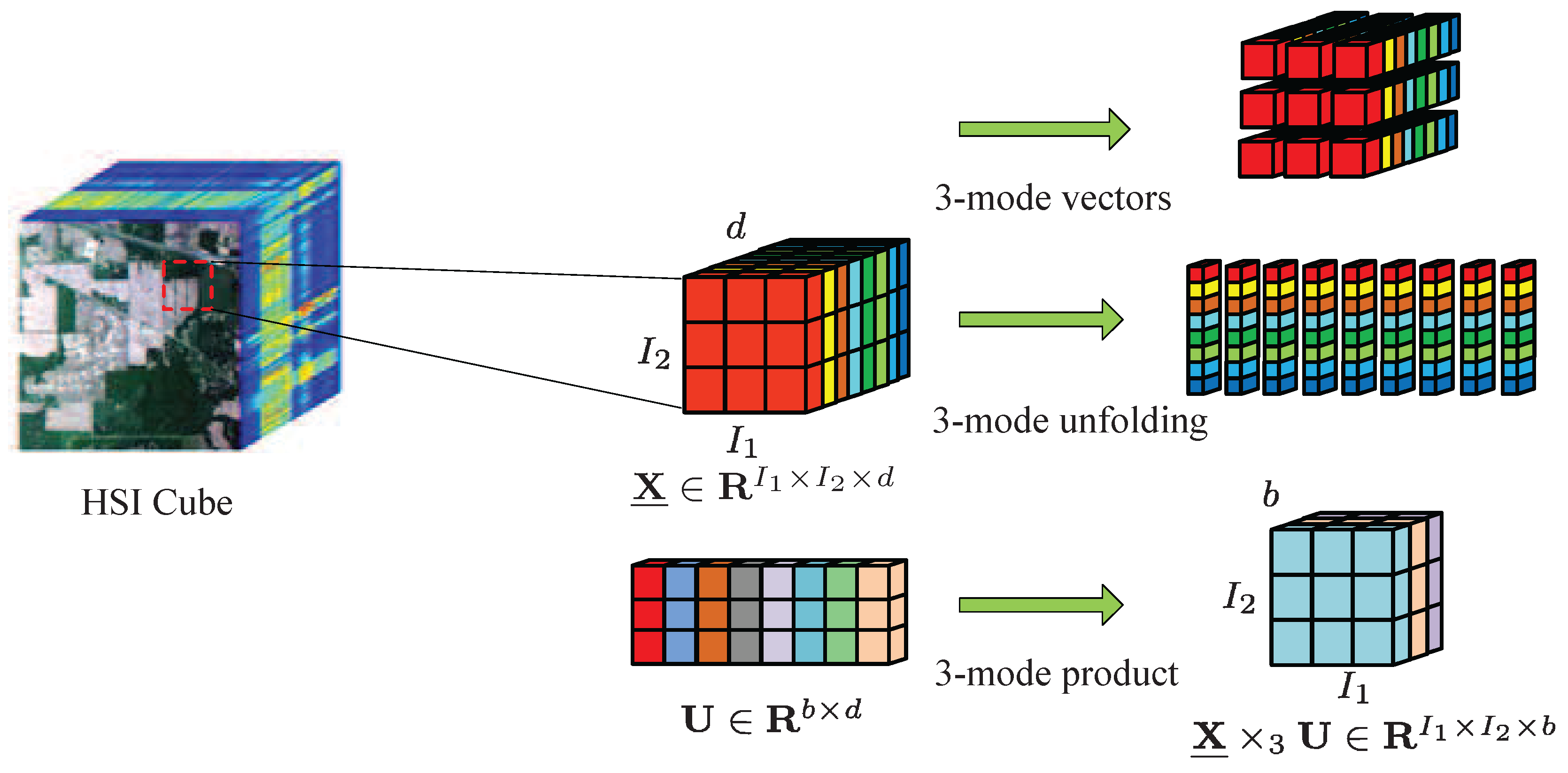
Consider a hyperspectral image as a third-order tensor , in which and refer to the width and height of the data cube, respectively, and represents the number of spectral bands, . Assume that the kth small patch is composed of the kth training sample and its neighbors, which is denoted as . M patches construct the training set . The training patches belonging to the lth class are expressed as , where represents the number of patches belonging to the lth class and . For the purpose of convenient expression, a fourth-order tensor is defined to represent these patches, and denotes all training patches for c classes, where . A visual illustration of 3-mode vectors, 3-mode unfolding, and 3-mode product is shown in Figure 1.
3.1. Tensor Sparse and Low-Rank Graph
The previous SLGDA framework can capture the local and global structure of hyperspectral data simultaneously by imposing both sparse and low-rank constraints. However, it may lose some important structural information of hyperspectral data, which presents an intrinsic tensor-based data structure. To overcome this drawback, a tensor sparse and low-rank graph is constructed with the objective function
where denotes the graph weigh matrix using labeled patches from the lth class only. As such, with the help of class-specific labeled training patches, the global graph weigh matrix can be designed as a block-diagonal structure
To obtain the lth class graph weight matrix , the alternating direction method of multipliers (ADMM) [35] is adopted to solve problem (12). Two auxiliary variables and are first introduced to make the objective function separable
The augmented Lagrangian function of problem (14) is given as
where and are Lagrangian multipliers, and is a penalty parameter.
By minimizing the function , each variable is alternately updated with other variables being fixed. The updating rules are expressed as
where denotes the learning rate, is the singular value thresholding operator (SVT), in which is the soft thresholding operator [36]. By fixing and , the formulation of can be written as
where , , and is an identity matrix.
The global similarity matrix will be obtained depending on Equation (13) when each sub-similarity matrix corresponding to each class is calculated from problem (12). Until now, a tensor sparse and low-rank graph is completely constructed with vertex set and similarity matrix . How to obtain a set of projection matrices is the following task.
3.2. Tensor Locality Preserving Projection
The aim of tensor LPP is to find transformation matrices to project high-dimensional data into low-dimensional representation , where .
The optimization problem for tensor LPP can be expressed as
where . It can be seen that the corresponding tensors and in the embedded tensor space are expected to be close to each other if original tensors and are greatly similar.
To solve the optimization problem (19), an iterative scheme is employed [33]. First, we assume that are known, then, let . With properties of tensor and trace, the objective function (19) is rewritten as
where denotes the n-mode unfolding of tensor . Finally, the optimal solution of problem (20) is the eigenvectors corresponding to the first smallest nonzero eigenvalues of the following generalized eigenvalue problem
Assume , , then, problem (21) can be transformed into
To solve this problem, the function embedded in the MATLAB software (R2013a, The MathWorks, Natick, Massachusetts, USA) is adopted, i.e., , and the eigenvectors in corresponding to the first smallest nonzero eigenvalues in are chosen to form the projection matrix. The other projection matrices can be obtained in a similar manner. The complete TSLGDA algorithm is outlined in Algorithm 1.
| Algorithm 1: Tensor Sparse and Low-Rank Graph-Based Discriminant Analysis for Classification. |
| Input: Training patches , testing patches , regularization parameters and , |
| reduced dimensionality . |
| Initialize: , , , , , , , |
| maxIter = 100, . |
| 1. for do |
| 2. repeat |
| 3. Compute , , and according to (16)–(18). |
| 4. Update the Lagrangian multipliers: |
| , . |
| 5. Update : , where |
| 6. Check convergence conditions: . |
| 7. . |
| 8. until convergence conditions are satisfied or maxIter. |
| 9. end for |
| 10. Construct the block-diagonal weight matrix according to (13). |
| 11. Compute the projection matrices according to (21). |
| 12. Compute the reduced features: |
| , . |
| 13. Determine the class label of by NN classifier. |
| 14. Output: The class labels of test patches. |
4. Experiments and Discussions
In this section, three hyperspectral datasets are used to verify the performance of the proposed method. The proposed TSLGDA algorithm is compared with some state-of-the-art approaches, including unsupervised methods (e.g., PCA [8], MPCA [25]) and supervised methods (e.g., LDA [9], LFDA [10], SGDA [19], GDA-SS [15], SLGDA [23], G-LTDA (local tensor discriminant analysis with Gabor filters) [29]). SGDA is implemented using the SPAMS (SPArse Modeling Software) toolbox [38]. The nearest neighbor classifier (NN classifier) is exploited to classify the projected features obtained by these DR methods. The class-specific accuracy , overall accuracy (OA), average accuracy (AA), and kappa coefficient () are reported for quantitative assessment after ten runs. All experiments are implemented on an Inter Core i5-4590 CPU personal computer (Santa Clara, CA, USA).
4.1. Experimental Datasets
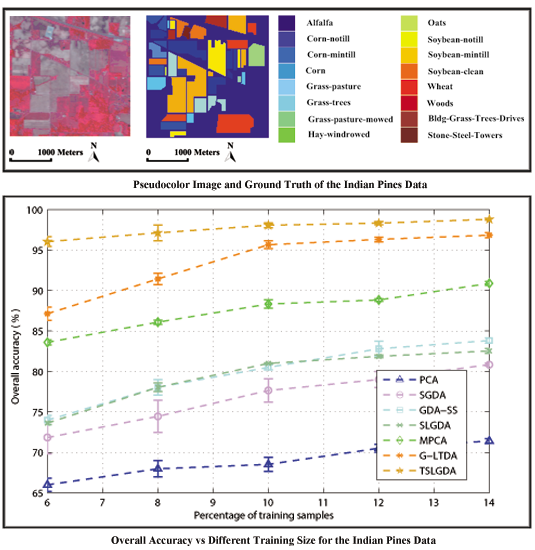
The first dataset [39] was acquired by Airborne Visible/Infrared Imaging Spectrometer (AVIRIS) sensor over northwest Indiana’s Indian Pine test site in June 1992. The AVIRIS sensor generates the wavelength range of 0.4–2.45-m covered 220 spectral bands. After removing 20 water-absorption bands (bands 104–108, 150–163, and 220), a total of 200 bands is used in experiments. The image with 145 × 145 pixels represents a rural scenario having 16 different land-cover classes. The numbers of training and testing samples in each class are listed in Table 1.
The second dataset [39] is the University of Pavia collected by the Reflective Optics System Imaging Spectrometer (ROSIS) sensor in Italy. The image has 103 bands after removing 12 noisy bands with a spectral coverage from 0.43 to 0.86 m, covering a region of 610 × 340 pixels. There are nine ground-truth classes, from which we randomly select training and testing samples as shown in Table 1.
The third dataset [39] was also collected by the AVIRIS sensor over the Valley of Salinas, Central Coast of California, in 1998. The image comprises 512 × 217 pixels with a spatial resolution of 3.7 m, and only preserves 204 bands after 20 water-absorption bands removed. Table 2 lists 16 land-cover classes and the number of training and testing samples.
4.2. Parameters Tuning
For the proposed method, four important parameters (i.e., regularization parameters and , window size, and the number of spectral dimension) that can be divided into three groups need to be determined before proceeding to the following experiments. and control the effect of sparse term and low-rank term in the objective function, respectively, which can be tuned together, while window size and the number of spectral dimension are another two groups that can be determined separately. When analyzing one group specific parameter, the other group parameters are fixed on their corresponding chosen values. According to many existing DR methods [22,23,24] and tensor-based research [26,28], window size is the first set as 9 for the Indian Pines and Salinas datasets, and 7 for the University of Pavia dataset; the initial value for the number of spectral dimension is given as 30 for all three datasets, and the performance basically reaches steady state with this dimension.
4.2.1. Regularization Parameters for TSLGDA
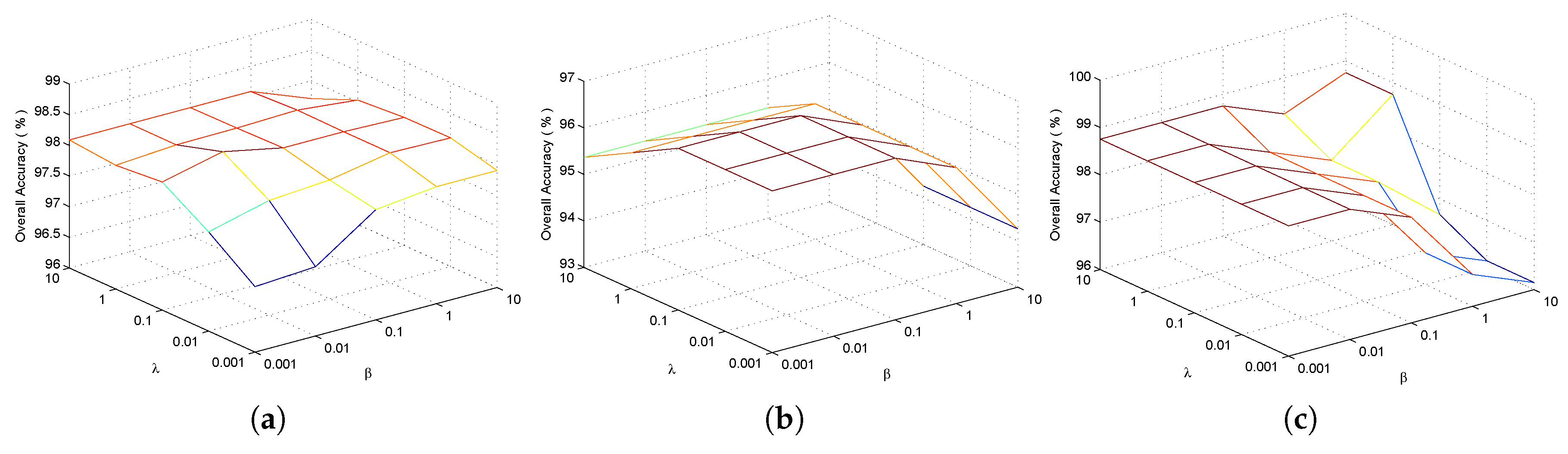
With the initial values of window size and the number of spectral dimension fixed, and are first tuned to achieve better classification performance. Figure 2 shows the overall classification accuracy with respect to different and by fivefold cross validation for three experimental datasets. It can be clearly seen that the OA values can reach the maximum values for some and . Accordingly, for the Indian Pines dataset, the optimal values of and can be set as , which is also an appropriate choice for the University of Pavia dataset, while is chosen for the Salinas data.
4.2.2. Window Size for Tensor Representation
For tensor-based DR methods, i.e., MPCA and TSLGDA, window size (or patch size) is another important parameter. Note that small windows may fail to cover enough spatial information, whereas large windows may contain multiple classes, resulting in complicated analysis and heavy computational burden. Therefore, the window size is searched in the range of . and are fixed on the tuned values, while the numbers of spectral dimension are still set as initial values for three datasets, respectively. Figure 3 presents the variation of classification performances of MPCA and TSLGDA with different window sizes for experimental datasets. It can be seen that the window sizes for MPCA and TSLGDA can be both chosen as for the Indian Pines and Salinas datasets, while the optimal values are and , respectively, for the University of Pavia dataset. This may be because the formers represent a rural scenario containing large spatial homogeneity while the Pavia University data is obtained from an urban area with small homogeneous regions. To evaluate the classification performance using the low-dimensional data, 1NN classifier is adopted in this paper.
4.2.3. The Number of Spectral Dimension for TSLGDA
According to [28], is set as the reduced dimensionality of the first two dimensions (i.e., two spatial dimensions). The third dimension (i.e., spectral dimension) is considered carefully by keeping the tuned values of , , and window size is fixed. Figure 4 shows the overall classification accuracy with respect to spectral dimension for three hyperspectral datasets. Obviously, due to the spatial information contained in tensor structure, tensor-based DR methods (i.e., MPCA, TSLGDA) outperform vector-based DR methods (i.e., PCA, SGDA, GDA-SS, SLGDA). According to [29,37], G-LTDA can automatically obtain the optimal reduced dimensions during the optimization procedure; therefore, the number of spectral dimension for G-LTDA is not discussed here. For the Indian Pines dataset, the performances of all considered methods increase when the spectral dimension increases, and then keep stable at the maximum values. The similar results can also be observed from the University of Pavia and Salinas datasets. In any case, TSLGDA outperforms other DR methods even when the spectral dimension is as low as 5. In the following assessment, and dimensions are used to conduct classification for two AVIRIS datasets and one ROSIS dataset, respectively.
4.3. Classification Results
4.3.1. Classification Accuracy
Table 3, Table 4 and Table 5 present the classification accuracy of individual class, OA, AA, and kappa coefficient for three experimental datasets, respectively. Obviously, the proposed method provides the best results than other compared methods on almost all of classes; meanwhile, OA, AA, and kappa coefficient are also better than those of other methods. Specifically, by comparing to all considered methods, TSLGDA yields about 2% to 30%, 5% to 20%, and 2% to 12% gain in OA with limited training sets for three datasets, respectively. Even for classes with few labeled training samples, such as class 1, class 7, and class 9 in the Indian Pines data, the proposed TSLGDA algorithm offers great improvement in performance as well. Besides TSLGDA, MPCA and G-LTDA also obtain much higher accuracies than other vector-based methods, which effectively demonstrates the advantage of tensor-based techniques. In addition, SLGDA yields better results than SGDA (about 3%, 1%, and 0.6% gain) by simultaneously exploiting the properties of sparsity and low-rankness, while GDA-SS is superior to SGDA by considering the spectral similarity measurement based on spectral characteristics when constructing the graph.
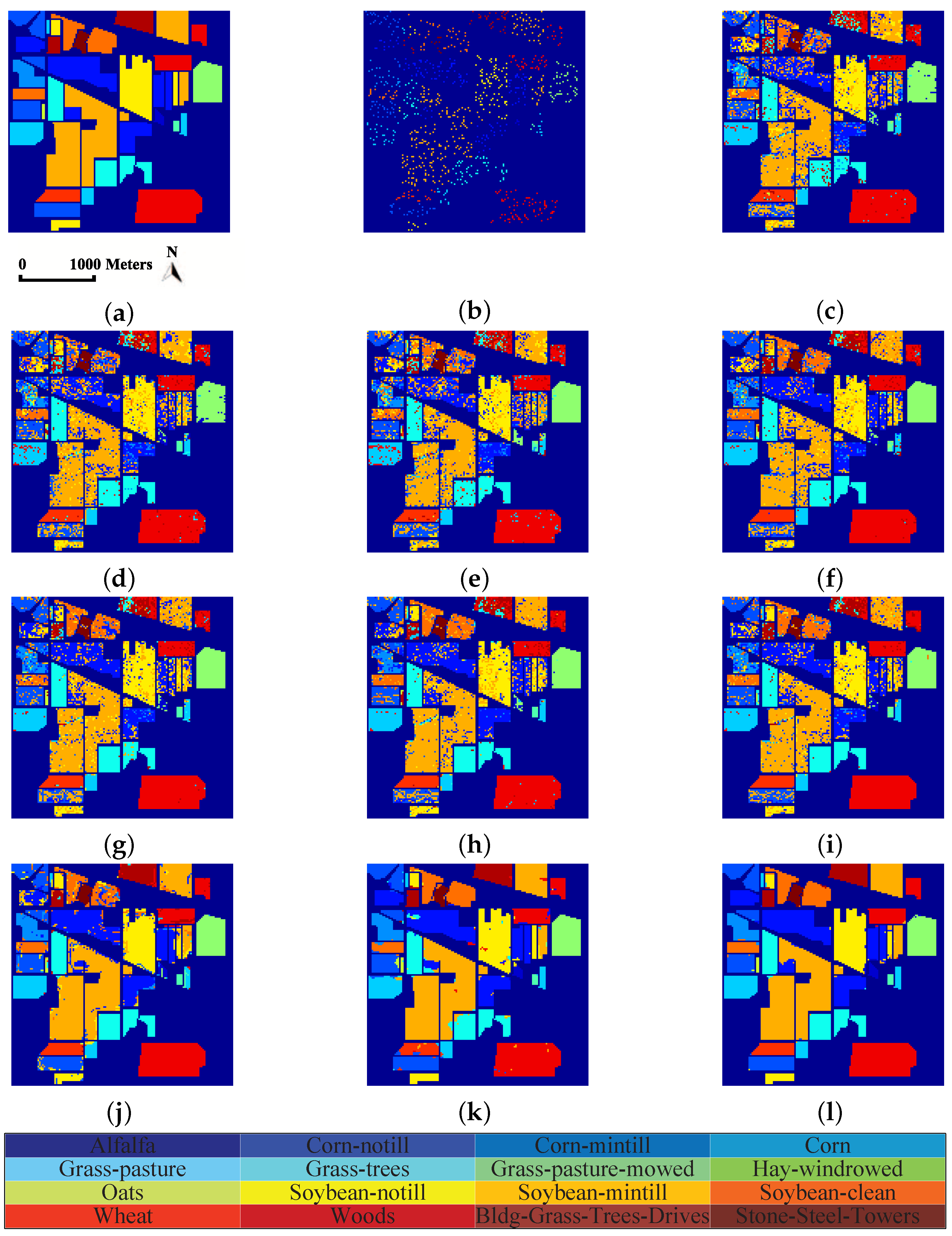
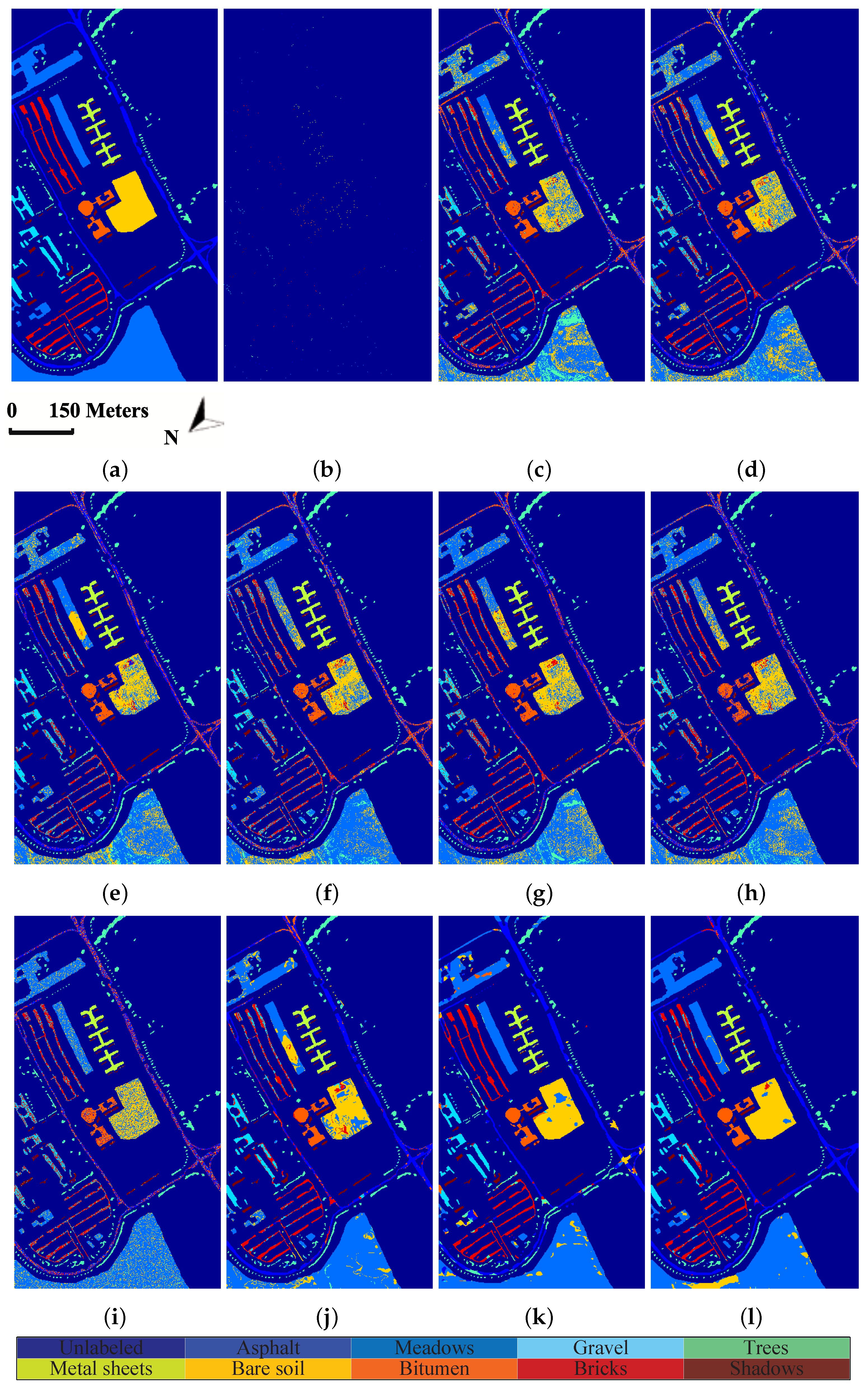
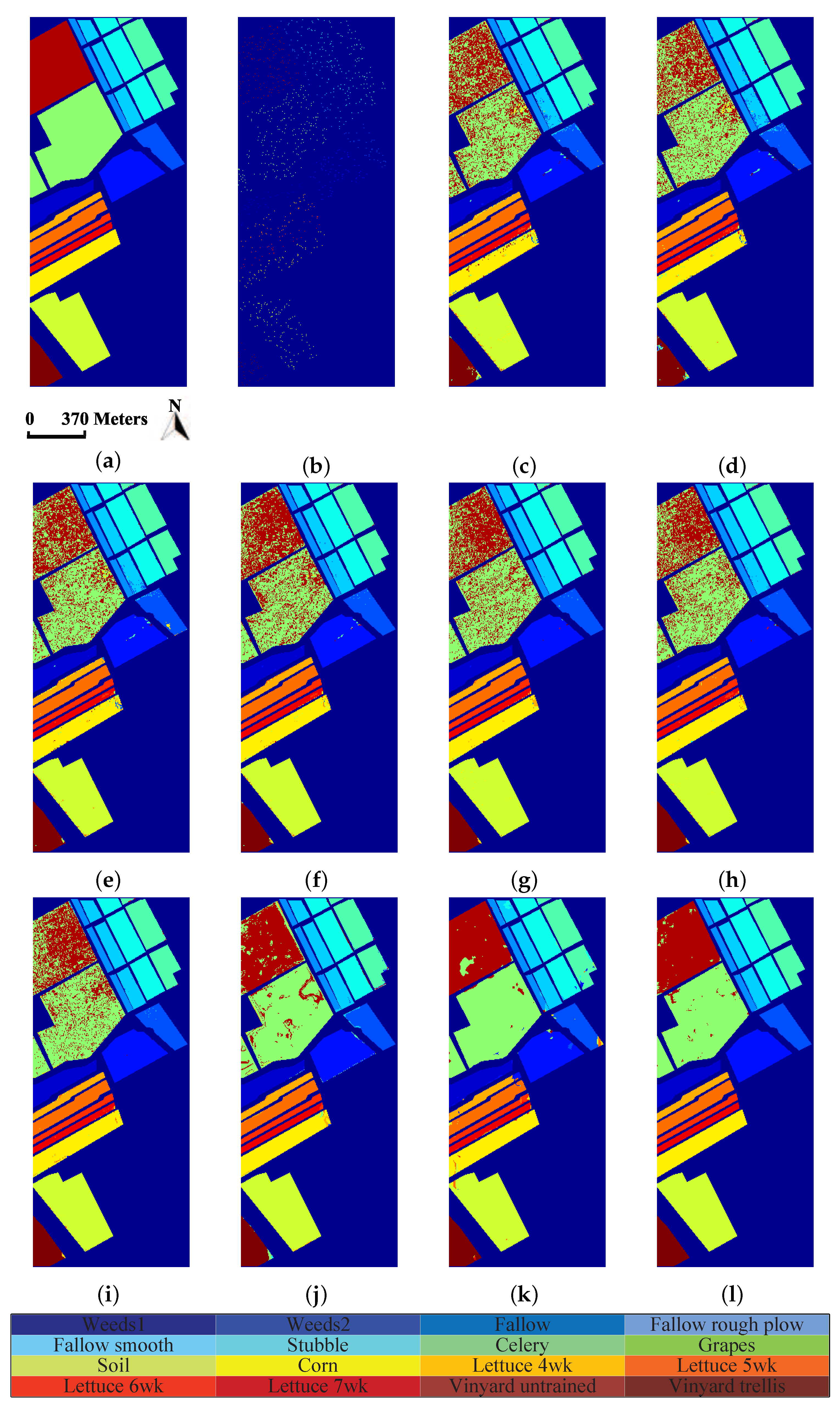
4.3.2. Classification Maps
In order to show the classification results more directly, classification maps of all considered methods are provided in Figure 5, Figure 6 and Figure 7 for three experimental datasets, respectively. From Figure 5, it can be clearly seen that the proposed method can obtain much smoother classification regions than other methods, especially for class 1 (Alfalfa), class 2 (Corn-notill), class 3 (Corn-mintill), and class 12 (Soybean-clean) whose spectral characteristics are highly correlated with other classes. The similar results can also be observed from Figure 6 and Figure 7, where class 1 (Asphalt), class 6 (Bare Soil), and class 8 (Self-blocking bricks) in the second dataset, and class 8 (Grapes untrained), class 15 (Vineyard untrained) in the third dataset are labeled more precisely. These observations are consistent with the quantitative results listed in Table 3, Table 4 and Table 5.
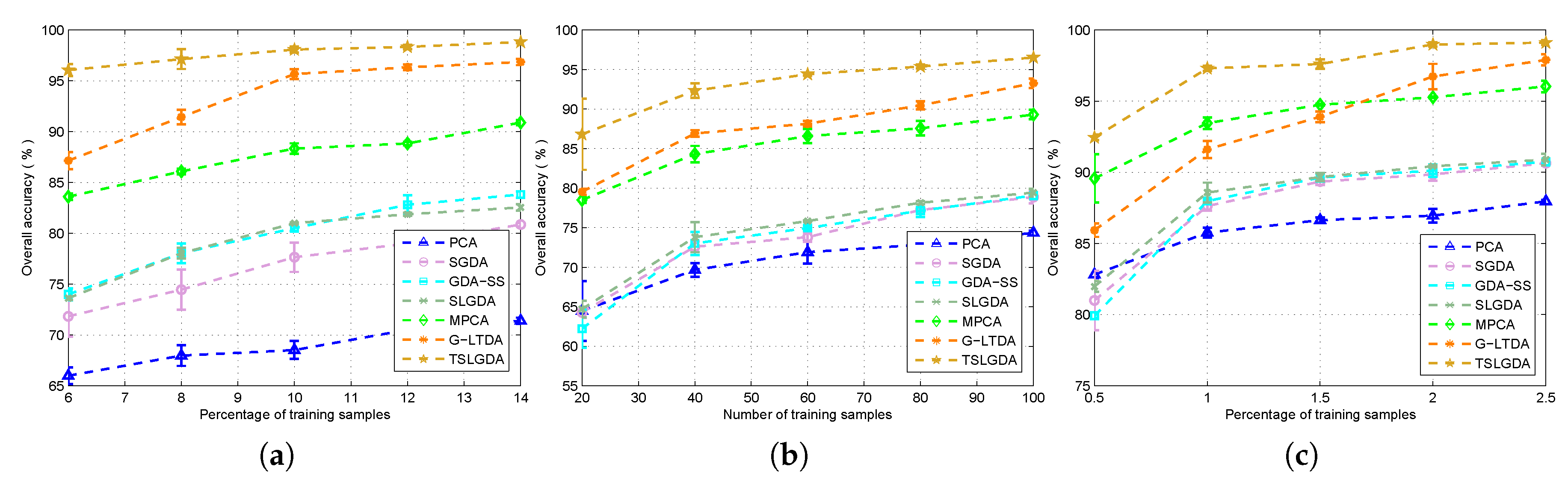
4.3.3. The Influence of Training Size
To show the influence of training size, some considered DR methods are tested. The results are given in Figure 8, from which we can see that the OA values of all methods are improved when the number of training samples increases for three datasets. Due to the spatial structure information contained in the tensor, the proposed method always performs better than other methods in all cases. In addition, with the label information, the supervised DR methods (i.e., SGDA, GDA-SS, SLGDA, G-LTDA, TSLGDA) achieve better results than the corresponding unsupervised DR methods (i.e., PCA, MPCA).
4.3.4. The Analysis of Computational Complexity
For the comparison of computational complexity, we take the Indian Pines data as an example. Table 6 shows the time requirements of all considered methods, from which it can be clearly seen that traditional methods (e.g., PCA, LDA, LFDA) run faster than other recently proposed methods. In addition, due to complicated tensor computation, tensor-based DR methods (e.g., MPCA, G-LTDA, TSLGDA) cost more time than vector-based methods (e.g., SGDA, GDA-SS, SLGDA). Although TSLGDA has the highest computational complexity, it yields the best classification performance. In practice, the general-purpose graphics processing units (GPUs) can be adopted to greatly accelerate the TSLGDA algorithm.
5. Conclusions
In this paper, we have proposed a tensor sparse and low-rank graph-based discriminant analysis method (i.e., TSLGDA) for dimensionality reduction of hyperspectral imagery. The hyperspectral data cube is taken as a third-order tensor, from which sub-tensors (local patches) centered at the training samples are extracted to construct the sparse and low-rank graph. On the one hand, by imposing both the sparse and low-rank constraints on the objective function, the proposed method is capable of capturing the local and global structure simultaneously. On the other hand, due to the spatial structure information introduced by tensor data, the proposed method can improve the graph structure and enhance the discriminative ability of reduced features. Experiments conducted on three hyperspectral datasets have consistently confirmed the effectiveness of our proposed TSLGDA algorithm, even for small training size. Compared to some state-of-the-art methods, the overall classification accuracy of TSLGDA in the low-dimensional space improves about 2% to 30%, 5% to 20%, and 2% to 12% for three experimental datasets, respectively, with increased computational complexity.
Acknowledgments
This work was supported by the National Natural Science Foundation of China under Grant 61371165 and Grant 61501018, and by the Frontier Intersection Basic Research Project for the Central Universities under Grant A0920502051714-5. The authors would like to thank Prof. David A. Landgreve from Purdue University for providing the AVIRIS image of Indian Pines and Prof. Paolo Gamba from University of Pavia for providing the ROSIS dataset. The authors would like to thank Dr. Zisha Zhong for sharing the code of Gabor filters and giving some useful suggestions. Last but not least, we would like to thank the editors and the anonymous reviewers for their detailed comments and suggestions, which greatly helped us to improve the clarity and presentation of our manuscript.
Author Contributions
All of the authors made significant contributions to the work. Lei Pan and Heng-Chao Li designed the research model, analyzed the results and wrote the paper. Yang-Jun Deng provided codes about tensor processing. Fan Zhang and Xiang-Dong Chen reviewed the manuscript. Qian Du contributed to the editing and review of the manuscript.
Conflicts of Interest
The authors declare no conflict of interest.
References
- He, Z.; Li, J.; Liu, L. Tensor block-sparsity based representation for spectral-spatial hyperspectral image classification. Remote Sens. 2016, 8, 636. [Google Scholar] [CrossRef]
- Peng, B.; Li, W.; Xie, X.M.; Du, Q.; Liu, K. Weighted-fusion-based representation classifiers for hyperspectral imagery. Remote Sens. 2015, 7, 14806–14826. [Google Scholar] [CrossRef]
- Yu, S.Q.; Jia, S.; Xu, C.Y. Convolutional neural networks for hyperspectral image classification. Neurocomputing 2017, 219, 88–98. [Google Scholar] [CrossRef]
- Jimenez, L.O.; Landgrebe, D.A. Supervised classification in high-dimensional space: Geometrical, statistical, and asymptoticla properitier of multivariate data. IEEE Trans. Syst. Man Cybern. Part C Appl. Rev. 1998, 28, 39–54. [Google Scholar] [CrossRef]
- Chang, C.-I.; Safavi, H. Progressive dimensionality reduction by transform for hyperspectral imagery. Pattern Recognit. 2011, 44, 2760–2773. [Google Scholar] [CrossRef]
- Yuan, Y.; Lin, J.Z.; Wang, Q. Dual-clustering-based hyperspectral band selection by contextual analysis. IEEE Trans. Geosci. Remote Sens. 2016, 54, 1431–1445. [Google Scholar] [CrossRef]
- Wang, Q.; Lin, J.Z.; Yuan, Y. Salient band selection for hyperspectral image classification via manifold ranking. IEEE Trans. Neural Netw. Learn. Syst. 2016, 27, 1279–1289. [Google Scholar] [CrossRef] [PubMed]
- Jolliffe, I.T. Principal Component Analysis; Springer-Verlag: New York, NY, USA, 2002. [Google Scholar]
- Bandos, T.V.; Bruzzone, L.; Camps-Valls, G. Classification of hyperspectral images with regularized linear discriminant analysis. IEEE Trans. Geosci. Remote Sens. 2009, 47, 862–873. [Google Scholar] [CrossRef]
- Li, W.; Prasad, S.; Fowler, J.E.; Bruce, L.M. Locality-preserving dimensionality reduction and classification for hyperspectral image analysis. IEEE Trans. Geosci. Remote Sens. 2012, 50, 1185–1198. [Google Scholar] [CrossRef]
- Tan, K.; Zhou, S.Y.; Du, Q. Semisupervised discriminant analysis for hyperspectral imagery with block-sparse graph. IEEE Geosci. Remote Sens. Lett. 2015, 12, 1765–1769. [Google Scholar] [CrossRef]
- Chatpatanasiri, R.; Kijsirikul, B. A unifier semi-supervised dimensionality reduction framework for manifold learning. Neurocomputing 2010, 73, 1631–1640. [Google Scholar] [CrossRef]
- Yan, S.C.; Xu, D.; Zhang, B.Y.; Zhang, H.-J.; Yang, Q.; Lin, S. Graph embedding and extensions: A general framework for dimensionality reduction. IEEE Trans. Pattern Anal. Mach. Intell. 2007, 29, 40–51. [Google Scholar] [CrossRef] [PubMed]
- He, X.F.; Cai, D.; Yan, S.C.; Zhang, H.-J. Neighborhood preserving embedding. In Proceedings of the 2005 IEEE Conference on Computer Vision (ICCV), Beijing, China, 17–20 October 2005; pp. 1208–1213. [Google Scholar]
- Feng, F.B.; Li, W.; Du, Q.; Zhang, B. Dimensionality reduction of hyperspectral image with graph-based discriminant analysis considering spectral similarity. Remote Sens. 2017, 9, 323. [Google Scholar] [CrossRef]
- Wright, J.; Yang, A.Y.; Ganesh, A.; Sastry, S.S.; Ma, Y. Robust face recognition via sparse representation. IEEE Trans. Pattern Anal. Mach. Intell. 2009, 31, 210–227. [Google Scholar] [CrossRef] [PubMed]
- Wright, J.; Ma, Y.; Mairal, J.; Sapiro, G.; Huang, T.S.; Yan, S.C. Sparse representation for computer vision and pattern recognition. Proc. IEEE 2010, 98, 1031–1044. [Google Scholar] [CrossRef]
- Cheng, B.; Yang, J.C.; Yan, S.C.; Fu, Y.; Huang, T.S. Learning with l1-graph for image analysis. IEEE Trans. Image Process. 2015, 23, 2241–2253. [Google Scholar]
- Ly, N.H.; Du, Q.; Fowler, J.E. Sparse graph-based discriminant analysis for hyperspectral imagery. IEEE Trans. Geosci. Remote Sens. 2014, 52, 3872–3884. [Google Scholar]
- He, W.; Zhang, H.Y.; Zhang, L.P.; Philips, W.; Liao, W.Z. Weighted sparse graph based dimensionality reduction for hyperspectral images. IEEE Geosci. Remote Sens. Lett. 2016, 13, 686–690. [Google Scholar] [CrossRef]
- Ly, N.H.; Du, Q.; Fowler, J.E. Collaborative graph-based discriminant analysis for hyperspectral imagery. IEEE J. Sel. Top. Appl. Earth Observ. Remote Sens. 2014, 7, 2688–2696. [Google Scholar] [CrossRef]
- Li, W.; Du, Q. Laplacian regularized collaborative graph for discriminant analysis of hyperspectral imagery. IEEE Trans. Geosci. Remote Sens. 2016, 54, 7066–7076. [Google Scholar] [CrossRef]
- Li, W.; Liu, J.B.; Du, Q. Sparse and low-rank graph for discriminant analysis of hyperspectral imagery. IEEE Trans. Geosci. Remote Sens. 2016, 54, 4094–4105. [Google Scholar] [CrossRef]
- Xue, Z.H.; Du, P.J.; Li, J.; Su, H.J. Simultaneous sparse graph embedding for hyperspectral image classification. IEEE Trans. Geosci. Remote Sens. 2015, 53, 6114–6132. [Google Scholar] [CrossRef]
- Lu, H.P.; Plataniotis, K.N.; Venetsanopoulos, A.N. MPCA: Multilinear principal component analysis of tensor objects. IEEE Trans. Neural Netw. 2008, 19, 18–39. [Google Scholar] [PubMed]
- Guo, X.; Huang, X.; Zhang, L.F.; Zhang, L.P.; Plaza, A.; Benediktssom, J.A. Support tensor machines for classification of hyperspectral remote sensing imagery. IEEE Trans. Geosci. Remote Sens. 2016, 54, 3248–3264. [Google Scholar] [CrossRef]
- An, J.L.; Zhang, X.R.; Jiao, L.C. Dimensionality reduction based on group-based tensor model for hyperspectral image classification. IEEE Geosci. Remote Sens. Lett. 2016, 13, 1497–1501. [Google Scholar] [CrossRef]
- Zhang, L.P.; Zhang, L.F.; Tao, D.C.; Huang, X. Tensor discriminative locality alignment for hyperspectral image spectral-spatial feature extraction. IEEE Trans. Geosci. Remote Sens. 2013, 51, 242–256. [Google Scholar] [CrossRef]
- Zhong, Z.S.; Fan, B.; Duan, J.Y.; Wang, L.F.; Ding, K.; Xiang, S.M.; Pan, C.H. Discriminant tensor spectral-spatial feature extraction for hyperspectral image classification. IEEE Geosci. Remote Sens. Lett. 2015, 12, 1028–1032. [Google Scholar] [CrossRef]
- Benediktsson, J.A.; Palmason, J.A.; Sveinsson, J.R. Classification of hyperspectral data from urban areas based on extended morphological profiles. IEEE Trans. Geosci. Remote Sens. 2005, 43, 480–491. [Google Scholar] [CrossRef]
- Dallal Mura, M.; Benediktsson, J.A.; Waske, B.; Bruzzone, L. Morphological attribute profiles for the analysis of very high resolution images. IEEE Trans. Geosci. Remote Sens. 2010, 48, 3747–3762. [Google Scholar] [CrossRef]
- Rajadell, O.; Garcia-Sevilla, P.; Pla, F. Spectral-spatial pixel characterization using Gabor filters for hyperspectral image classification. IEEE Geosci. Remote Sens. Lett. 2013, 10, 860–864. [Google Scholar] [CrossRef]
- Zhao, H.T.; Sun, S.Y. Sparse tensor embedding based multispectral face recognition. Neurocomputing 2014, 133, 427–436. [Google Scholar] [CrossRef]
- Lai, Z.H.; Xu, Y.; Chen, Q.C.; Yang, J.; Zhang, D. Multilinear sparse principal component analysis. IEEE Trans. Neural Netw. Learn. Syst. 2014, 25, 1942–1950. [Google Scholar] [CrossRef] [PubMed]
- Boyd, S.; Parikh, N.; Chu, E.; Peleato, B.; Eckstein, J. Distributed optimization and statistical learning via the alternating direction method of multipliers. Found. Trends Mach. Learn. 2011, 3, 1–122. [Google Scholar] [CrossRef]
- Cai, J.-F.; Candés, E.J.; Shen, Z. A singular value thresholding algorithm for matrix completion. SIAM J. Optim. 2010, 24, 1956–1982. [Google Scholar] [CrossRef]
- Nie, F.P.; Xiang, S.M.; Song, Y.Q.; Zhang, C.S. Extracting the optimal dimensionality for local tensor discriminant analysis. Pattern Recognit. 2009, 42, 105–114. [Google Scholar] [CrossRef]
- SPArse Modeling Software. Available online: http://spams-devel.gforge.inria.fr/index.html (accessed on 20 January 2017).
- Hyperspectral Remote Sensing Scenes. Available online: http://www.ehu.eus/ccwintco/index.php?title=Hyperspectral_Remote_Sensing_Scenes (accessed on 20 January 2017).
Figure 1.
Visual illustration of n-mode vectors, n-mode unfolding, and n-mode product of a third-order tensor from a hyperspectral image.
Figure 1.
Visual illustration of n-mode vectors, n-mode unfolding, and n-mode product of a third-order tensor from a hyperspectral image.

Figure 2.
Parameter tuning of and for the proposed TSLGDA algorithm using three datasets: (a) Indian Pines; (b) University of Pavia; (c) Salinas.
Figure 2.
Parameter tuning of and for the proposed TSLGDA algorithm using three datasets: (a) Indian Pines; (b) University of Pavia; (c) Salinas.

Figure 3.
Parameter tuning of window size for MPCA and TSLGDA using three datasets: (a) Indian Pines; (b) University of Pavia; (c) Salinas.
Figure 3.
Parameter tuning of window size for MPCA and TSLGDA using three datasets: (a) Indian Pines; (b) University of Pavia; (c) Salinas.

Figure 4.
Overall accuracy versus the reduced spectral dimension for different methods using three datasets: (a) Indian Pines; (b) University of Pavia; (c) Salinas.
Figure 4.
Overall accuracy versus the reduced spectral dimension for different methods using three datasets: (a) Indian Pines; (b) University of Pavia; (c) Salinas.
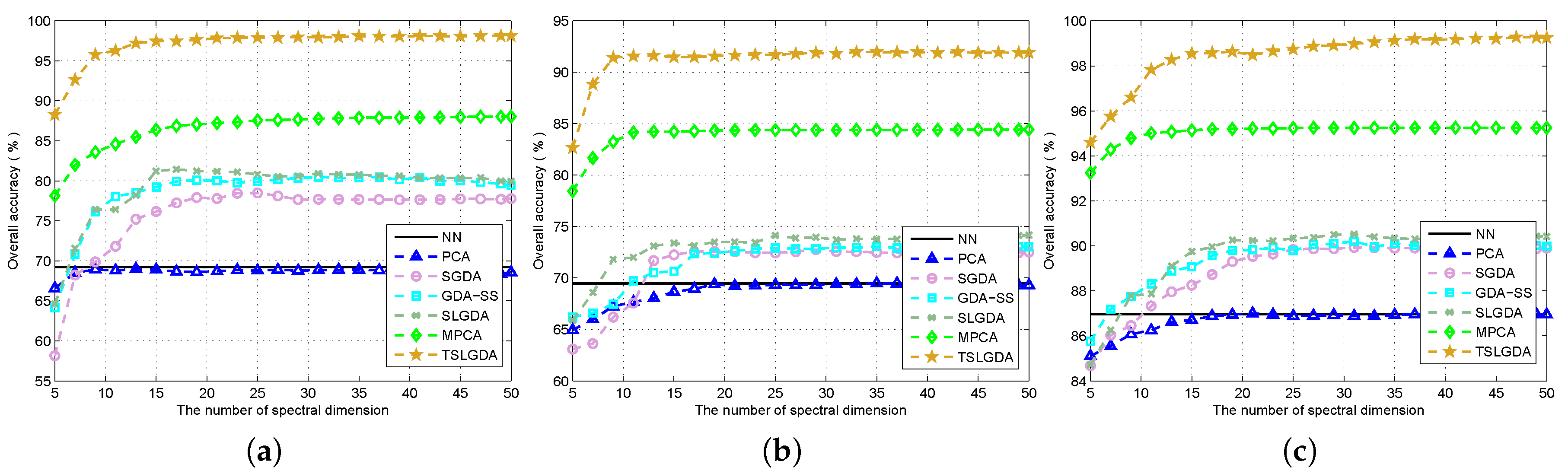
Figure 5.
Classification maps of different methods for the Indian Pines dataset: (a) ground truth; (b) training set; (c) origin; (d) PCA; (e) LDA; (f) LFDA; (g) SGDA; (h) GDA-SS; (i) SLGDA; (j) MPCA; (k) G-LTDA; and (l) TSLGDA.
Figure 5.
Classification maps of different methods for the Indian Pines dataset: (a) ground truth; (b) training set; (c) origin; (d) PCA; (e) LDA; (f) LFDA; (g) SGDA; (h) GDA-SS; (i) SLGDA; (j) MPCA; (k) G-LTDA; and (l) TSLGDA.

Figure 6.
Classification maps of different methods for the University of Pavia dataset: (a) ground truth; (b) training set; (c) origin; (d) PCA; (e) LDA; (f) LFDA; (g) SGDA; (h) GDA-SS; (i) SLGDA; (j) MPCA; (k) G-LTDA; and (l) TSLGDA.
Figure 6.
Classification maps of different methods for the University of Pavia dataset: (a) ground truth; (b) training set; (c) origin; (d) PCA; (e) LDA; (f) LFDA; (g) SGDA; (h) GDA-SS; (i) SLGDA; (j) MPCA; (k) G-LTDA; and (l) TSLGDA.

Figure 7.
Classification maps of different methods for the Salinas dataset: (a) ground truth; (b) training set; (c) origin; (d) PCA; (e) LDA; (f) LFDA; (g) SGDA; (h) GDA-SS; (i) SLGDA; (j) MPCA; (k) G-LTDA; and (l) TSLGDA.
Figure 7.
Classification maps of different methods for the Salinas dataset: (a) ground truth; (b) training set; (c) origin; (d) PCA; (e) LDA; (f) LFDA; (g) SGDA; (h) GDA-SS; (i) SLGDA; (j) MPCA; (k) G-LTDA; and (l) TSLGDA.

Figure 8.
Overall classification accuracy and standard deviation versus different numbers of training samples per class for all methods using three datasets: (a) Indian Pines; (b) University of Pavia; (c) Salinas.
Figure 8.
Overall classification accuracy and standard deviation versus different numbers of training samples per class for all methods using three datasets: (a) Indian Pines; (b) University of Pavia; (c) Salinas.


Table 1.
Number of training and testing samples for the Indian Pines and University of Pavia datasets.
Table 1.
Number of training and testing samples for the Indian Pines and University of Pavia datasets.
| Indian Pines | University of Pavia | |||||
|---|---|---|---|---|---|---|
| Class | Name | Training | Testing | Name | Training | Testing |
| 1 | Alfalfa | 5 | 41 | Asphalt | 40 | 6591 |
| 2 | Corn-notill | 143 | 1285 | Meadows | 40 | 18,609 |
| 3 | Corn-mintill | 83 | 747 | Gravel | 40 | 2059 |
| 4 | Corn | 24 | 213 | Tree | 40 | 3024 |
| 5 | Grass-pasture | 48 | 435 | Painted metal sheets | 40 | 1305 |
| 6 | Grass-trees | 73 | 657 | Bare Soil | 40 | 4989 |
| 7 | Grass-pasture-mowed | 3 | 25 | Bitumen | 40 | 1290 |
| 8 | Hay-windrowed | 48 | 430 | Self-blocking bricks | 40 | 3642 |
| 9 | Oats | 2 | 18 | Shadows | 40 | 907 |
| 10 | Soybean-notill | 97 | 875 | |||
| 11 | Soybean-mintill | 246 | 2209 | |||
| 12 | Soybean-clean | 59 | 534 | |||
| 13 | Wheat | 21 | 184 | |||
| 14 | Woods | 127 | 1138 | |||
| 15 | Buildings-Grass-Trees-Drive | 39 | 347 | |||
| 16 | Stone-Steel-Towers | 9 | 84 | |||
| Total | 1027 | 9222 | 360 | 42,416 | ||
Table 2.
Number of training and testing samples for the Salinas dataset.
| Salinas | |||
|---|---|---|---|
| Class | Name | Training | Testing |
| 1 | Brocoli-green-weeds-1 | 40 | 1969 |
| 2 | Brocoli-green-weeds-2 | 75 | 3651 |
| 3 | Fallow | 40 | 1936 |
| 4 | Fallow-rough-plow | 28 | 1366 |
| 5 | Fallow-smooth | 54 | 2624 |
| 6 | Stubble | 79 | 3880 |
| 7 | Celery | 72 | 3507 |
| 8 | Grapes-untrained | 225 | 11,046 |
| 9 | Soil-vinyard-develop | 124 | 6079 |
| 10 | Corn-senesced-green-weeds | 66 | 3212 |
| 11 | Lettuce-romaine-4wk | 21 | 1047 |
| 12 | Lettuce-romaine-5wk | 39 | 1888 |
| 13 | Lettuce-romaine-6wk | 18 | 898 |
| 14 | Lettuce-romaine-7wk | 21 | 1049 |
| 15 | Vinyard-untrained | 145 | 7123 |
| 16 | Vinyard-vertical-trellis | 36 | 1771 |
| Total | 1083 | 53,046 | |
Table 3.
Classification accuracy (%) and standard deviation of different methods for the Indian Pines data when the reduced dimension is 30.
Table 3.
Classification accuracy (%) and standard deviation of different methods for the Indian Pines data when the reduced dimension is 30.
| No. | Origin | PCA | LDA | LFDA | SGDA | GDA-SS | SLGDA | MPCA | G-LTDA | TSLGDA |
|---|---|---|---|---|---|---|---|---|---|---|
| 1 | 39.02 | 54.15 | 33.66 | 44.88 | 65.04 | 49.59 | 48.78 | 71.34 | 92.20 | 91.71 |
| ±8.27 | ±11.1 | ±17.8 | ±15.5 | ±7.45 | ±12.2 | ±6.90 | ±9.63 | ±4.69 | ±8.02 | |
| 2 | 55.92 | 52.96 | 57.28 | 67.78 | 69.31 | 74.24 | 73.04 | 81.09 | 96.47 | 97.32 |
| ±2.68 | ±1.53 | ±2.13 | ±3.56 | ±2.37 | ±3.95 | ±1.93 | ±2.74 | ±1.01 | ±0.68 | |
| 3 | 49.83 | 50.15 | 58.34 | 66.75 | 62.65 | 69.57 | 67.00 | 82.26 | 93.98 | 97.51 |
| ±2.68 | ±2.34 | ±2.57 | ±2.82 | ±1.76 | ±5.56 | ±0.28 | ±2.74 | ±2.34 | ±0.91 | |
| 4 | 42.07 | 40.19 | 38.12 | 54.93 | 49.14 | 58.06 | 62.68 | 87.91 | 96.53 | 97.37 |
| ±7.75 | ±4.56 | ±4.00 | ±7.69 | ±5.40 | ±8.24 | ±12.3 | ±4.65 | ±3.93 | ±1.90 | |
| 5 | 82.95 | 84.47 | 81.20 | 88.25 | 89.55 | 92.03 | 93.32 | 91.13 | 93.15 | 97.00 |
| ±2.93 | ±4.58 | ±3.87 | ±2.41 | ±1.74 | ±1.34 | ±0.98 | ±2.00 | ±1.44 | ±2.50 | |
| 6 | 90.75 | 93.06 | 93.36 | 94.64 | 95.38 | 96.91 | 96.27 | 97.53 | 94.76 | 99.27 |
| ±1.00 | ±2.95 | ±1.47 | ±1.59 | ±0.61 | ±0.89 | ±0.11 | ±1.14 | ±2.94 | ±0.46 | |
| 7 | 81.60 | 72.00 | 76.00 | 79.20 | 88.00 | 88.00 | 88.00 | 94.00 | 95.20 | 96.80 |
| ±8.29 | ±13.6 | ±12.3 | ±22.5 | ±4.00 | ±8.00 | ±5.66 | ±7.66 | ±7.15 | ±3.35 | |
| 8 | 96.28 | 93.02 | 95.26 | 99.12 | 99.53 | 97.91 | 99.19 | 98.37 | 97.81 | 99.86 |
| ±1.78 | ±1.52 | ±2.71 | ±1.47 | ±0.40 | ±2.02 | ±0.49 | ±1.66 | ±0.67 | ±0.31 | |
| 9 | 26.67 | 34.44 | 25.56 | 43.33 | 50.00 | 37.04 | 25.00 | 54.17 | 78.89 | 93.33 |
| ±4.65 | ±12.0 | ±16.5 | ±9.94 | ±33.8 | ±16.9 | ±11.8 | ±19.4 | ±15.4 | ±7.24 | |
| 10 | 66.06 | 63.91 | 65.40 | 69.04 | 69.64 | 73.64 | 74.03 | 84.12 | 95.93 | 96.52 |
| ±2.04 | ±3.49 | ±3.61 | ±3.05 | ±5.81 | ±3.02 | ±0.32 | ±1.32 | ±1.35 | ±1.56 | |
| 11 | 71.75 | 71.41 | 73.65 | 72.43 | 78.18 | 79.45 | 79.52 | 90.30 | 96.32 | 98.53 |
| ±3.00 | ±2.00 | ±1.81 | ±1.83 | ±1.42 | ±1.23 | ±2.08 | ±0.78 | ±1.41 | ±0.59 | |
| 12 | 43.41 | 41.46 | 48.63 | 67.20 | 67.29 | 74.78 | 76.83 | 73.73 | 93.60 | 96.17 |
| ±6.34 | ±2.55 | ±3.25 | ±1.56 | ±2.19 | ±4.59 | ±1.99 | ±2.38 | ±1.70 | ±1.75 | |
| 13 | 91.41 | 94.02 | 93.59 | 98.70 | 96.01 | 97.83 | 98.64 | 98.23 | 91.85 | 99.46 |
| ±2.44 | ±2.40 | ±1.11 | ±0.62 | ±0.63 | ±1.63 | ±1.15 | ±1.12 | ±4.21 | ±0.67 | |
| 14 | 90.04 | 89.65 | 89.44 | 93.83 | 94.58 | 94.00 | 96.05 | 95.78 | 97.72 | 99.67 |
| ±1.96 | ±2.10 | ±2.16 | ±1.56 | ±0.89 | ±1.18 | ±0.87 | ±0.40 | ±0.66 | ±0.43 | |
| 15 | 37.98 | 36.54 | 41.15 | 61.04 | 48.90 | 56.20 | 56.48 | 88.26 | 95.91 | 98.67 |
| ±2.18 | ±2.30 | ±3.73 | ±2.89 | ±1.92 | ±3.20 | ±2.85 | ±4.69 | ±1.62 | ±1.16 | |
| 16 | 88.43 | 88.67 | 91.08 | 89.64 | 92.37 | 91.27 | 93.98 | 93.07 | 84.29 | 97.35 |
| ±6.30 | ±3.02 | ±3.47 | ±5.56 | ±3.03 | ±2.99 | ±1.70 | ±4.33 | ±8.68 | ±1.32 | |
| OA | 69.25 | 68.52 | 70.86 | 76.60 | 77.65 | 80.51 | 80.76 | 88.34 | 95.67 | 98.08 |
| ±1.16 | ±0.88 | ±0.76 | ±0.82 | ±1.44 | ±0.31 | ±0.08 | ±0.51 | ±0.49 | ±0.30 | |
| AA | 65.89 | 66.26 | 66.36 | 74.42 | 75.97 | 76.91 | 76.80 | 86.33 | 93.41 | 97.28 |
| ±1.19 | ±1.62 | ±2.30 | ±1.79 | ±2.37 | ±2.38 | ±1.98 | ±1.17 | ±0.56 | ±0.85 | |
| 64.90 | 64.04 | 66.73 | 73.32 | 74.40 | 77.70 | 78.01 | 86.70 | 95.07 | 97.81 | |
| ±1.30 | ±0.98 | ±0.92 | ±0.93 | ±1.68 | ±0.38 | ±0.14 | ±0.59 | ±0.56 | ±0.34 |
Table 4.
Classification accuracy (%) and standard deviation of different methods for the University of Pavia data when the reduced dimension is 20.
Table 4.
Classification accuracy (%) and standard deviation of different methods for the University of Pavia data when the reduced dimension is 20.
| No. | Origin | PCA | LDA | LFDA | SGDA | GDA-SS | SLGDA | MPCA | G-LTDA | TSLGDA |
|---|---|---|---|---|---|---|---|---|---|---|
| 1 | 56.13 | 55.98 | 64.77 | 60.56 | 47.44 | 52.88 | 52.84 | 84.20 | 72.41 | 91.15 |
| ±1.99 | ±2.90 | ±2.11 | ±5.24 | ±2.00 | ±6.58 | ±1.98 | ±1.49 | ±2.03 | ±1.46 | |
| 2 | 69.68 | 70.30 | 68.75 | 77.05 | 82.15 | 78.88 | 80.92 | 84.60 | 89.24 | 92.59 |
| ±5.59 | ±3.27 | ±3.44 | ±4.42 | ±2.71 | ±2.80 | ±3.74 | ±3.31 | ±0.93 | ±2.68 | |
| 3 | 68.02 | 67.34 | 69.90 | 66.47 | 63.83 | 64.27 | 61.17 | 80.24 | 89.48 | 86.83 |
| ±3.95 | ±1.49 | ±3.10 | ±3.94 | ±10.5 | ±3.28 | ±3.26 | ±3.01 | ±5.68 | ±2.44 | |
| 4 | 90.21 | 86.98 | 88.92 | 91.33 | 90.73 | 91.26 | 92.54 | 92.20 | 71.28 | 96.04 |
| ±4.43 | ±3.70 | ±2.23 | ±2.01 | ±2.25 | ±2.10 | ±0.07 | ±1.85 | ±4.90 | ±2.23 | |
| 5 | 99.39 | 99.49 | 99.51 | 99.88 | 99.73 | 99.79 | 99.66 | 99.72 | 98.41 | 100 |
| ±0.38 | ±0.23 | ±0.25 | ±0.10 | ±0.18 | ±0.08 | ±0.27 | ±0.26 | ±1.10 | ±0.00 | |
| 6 | 59.11 | 61.68 | 66.35 | 65.36 | 59.47 | 65.07 | 63.97 | 77.99 | 95.04 | 93.06 |
| ±2.25 | ±6.60 | ±6.62 | ±7.09 | ±5.18 | ±2.72 | ±0.50 | ±4.68 | ±2.35 | ±3.12 | |
| 7 | 83.36 | 83.22 | 86.34 | 75.78 | 82.25 | 79.04 | 81.71 | 89.22 | 98.26 | 97.50 |
| ±4.59 | ±3.57 | ±2.25 | ±1.97 | ±5.40 | ±3.64 | ±1.75 | ±2.09 | ±1.37 | ±0.90 | |
| 8 | 68.06 | 66.89 | 68.24 | 60.81 | 61.16 | 64.67 | 65.46 | 76.30 | 93.31 | 86.07 |
| ±2.72 | ±4.34 | ±3.24 | ±4.18 | ±8.92 | ±4.21 | ±2.87 | ±3.07 | ±1.32 | ±3.27 | |
| 9 | 95.94 | 95.90 | 97.00 | 83.95 | 84.04 | 87.81 | 85.17 | 99.49 | 88.00 | 98.39 |
| ±1.52 | ±1.36 | ±1.82 | ±4.64 | ±6.01 | ±2.20 | ±1.01 | ±0.32 | ±2.23 | ±1.03 | |
| OA | 69.47 | 69.65 | 71.38 | 73.04 | 72.59 | 73.01 | 73.80 | 84.30 | 86.92 | 92.33 |
| ±2.16 | ±0.88 | ±1.10 | ±0.70 | ±0.68 | ±1.47 | ±1.91 | ±1.05 | ±0.42 | ±0.93 | |
| AA | 76.66 | 76.42 | 78.86 | 75.69 | 74.53 | 75.96 | 75.94 | 87.11 | 88.38 | 93.52 |
| ±0.52 | ±0.70 | ±0.92 | ±1.55 | ±1.82 | ±0.74 | ±0.25 | ±0.71 | ±0.43 | ±0.53 | |
| 61.22 | 61.43 | 63.79 | 65.31 | 64.39 | 65.22 | 66.10 | 79.57 | 82.88 | 89.93 | |
| ±2.30 | ±0.88 | ±1.19 | ±0.83 | ±0.89 | ±1.74 | ±2.14 | ±1.24 | ±0.50 | ±1.17 |
Table 5.
Classification accuracy (%) and standard deviation of different methods for the Salinas data when the reduced dimension is 30.
Table 5.
Classification accuracy (%) and standard deviation of different methods for the Salinas data when the reduced dimension is 30.
| No. | Origin | PCA | LDA | LFDA | SGDA | GDA-SS | SLGDA | MPCA | G-LTDA | TSLGDA |
|---|---|---|---|---|---|---|---|---|---|---|
| 1 | 98.07 | 98.73 | 98.98 | 99.44 | 99.49 | 99.39 | 99.61 | 98.00 | 96.94 | 99.92 |
| ±0.44 | ±0.80 | ±0.81 | ±0.10 | ±0.13 | ±0.14 | ±0.23 | ±0.98 | ±1.63 | ±0.15 | |
| 2 | 98.68 | 98.90 | 98.88 | 99.23 | 99.54 | 99.25 | 99.50 | 99.47 | 98.73 | 99.98 |
| ±0.38 | ±0.25 | ±0.29 | ±0.17 | ±0.28 | ±0.21 | ±0.37 | ±0.55 | ±0.81 | ±0.03 | |
| 3 | 96.20 | 96.85 | 95.13 | 99.16 | 99.28 | 99.59 | 99.57 | 98.17 | 93.65 | 99.97 |
| ±0.25 | ±0.61 | ±1.05 | ±0.25 | ±0.05 | ±0.15 | ±0.17 | ±0.19 | ±1.88 | ±0.06 | |
| 4 | 99.24 | 99.39 | 99.51 | 99.12 | 99.41 | 99.12 | 99.15 | 99.71 | 93.92 | 98.41 |
| ±0.08 | ±0.35 | ±0.18 | ±0.46 | ±0.13 | ±0.41 | ±0.30 | ±0.87 | ±3.27 | ±0.68 | |
| 5 | 94.55 | 93.45 | 95.63 | 98.79 | 98.64 | 98.42 | 99.03 | 97.95 | 96.50 | 98.87 |
| ±0.66 | ±1.85 | ±0.81 | ±0.09 | ±0.87 | ±0.62 | ±0.12 | ±1.28 | ±1.76 | ±1.33 | |
| 6 | 99.67 | 99.63 | 99.56 | 99.79 | 99.77 | 99.70 | 99.87 | 99.24 | 98.74 | 100 |
| ±0.16 | ±0.25 | ±0.11 | ±0.21 | ±0.05 | ±0.13 | ±0.13 | ±1.27 | ±0.52 | ±0.00 | |
| 7 | 98.87 | 99.40 | 99.34 | 99.43 | 99.44 | 99.64 | 99.64 | 98.18 | 96.21 | 99.99 |
| ±0.53 | ±0.11 | ±0.24 | ±0.24 | ±0.09 | ±0.30 | ±0.08 | ±0.35 | ±2.39 | ±0.02 | |
| 8 | 72.41 | 73.59 | 74.13 | 73.01 | 76.25 | 78.11 | 78.86 | 90.80 | 97.93 | 97.73 |
| ±2.03 | ±2.33 | ±0.49 | ±3.40 | ±4.74 | ±0.42 | ±1.50 | ±0.19 | ±0.60 | ±0.22 | |
| 9 | 97.82 | 97.91 | 98.79 | 98.92 | 99.10 | 98.78 | 99.65 | 99.54 | 98.71 | 100 |
| ±0.01 | ±0.88 | ±0.50 | ±0.18 | ±0.19 | ±1.46 | ±0.12 | ±0.07 | ±1.07 | ±0.00 | |
| 10 | 87.70 | 89.62 | 91.68 | 95.24 | 96.07 | 94.88 | 95.42 | 94.77 | 94.96 | 99.77 |
| ±4.21 | ±0.33 | ±1.05 | ±0.44 | ±1.28 | ±1.65 | ±1.12 | ±0.67 | ±2.25 | ±0.37 | |
| 11 | 93.82 | 96.85 | 93.47 | 95.03 | 96.49 | 95.61 | 97.29 | 94.58 | 90.58 | 100 |
| ±1.38 | ±1.92 | ±4.81 | ±2.28 | ±3.75 | ±2.83 | ±3.54 | ±1.72 | ±4.90 | ±0.00 | |
| 12 | 99.75 | 99.93 | 99.45 | 99.95 | 99.91 | 99.95 | 99.82 | 99.44 | 97.17 | 100 |
| ±0.16 | ±0.12 | ±0.46 | ±0.09 | ±0.06 | ±0.07 | ±0.17 | ±0.98 | ±1.53 | ±0.00 | |
| 13 | 97.29 | 96.14 | 97.14 | 98.36 | 97.84 | 97.94 | 98.59 | 99.74 | 95.01 | 100 |
| ±0.17 | ±1.56 | ±0.17 | ±0.73 | ±0.89 | ±0.08 | ±0.84 | ±0.28 | ±2.11 | ±0.00 | |
| 14 | 92.49 | 93.89 | 95.00 | 94.91 | 96.91 | 95.23 | 97.23 | 94.97 | 93.16 | 99.87 |
| ±1.53 | ±0.87 | ±0.98 | ±1.63 | ±1.39 | ±2.02 | ±0.25 | ±2.23 | ±5.57 | ±0.15 | |
| 15 | 62.04 | 58.38 | 64.37 | 69.36 | 67.05 | 67.51 | 66.31 | 88.63 | 96.22 | 96.77 |
| ±1.48 | ±2.25 | ±1.98 | ±4.08 | ±5.23 | ±1.65 | ±1.88 | ±0.62 | ±1.10 | ±1.47 | |
| 16 | 94.75 | 94.44 | 98.00 | 98.78 | 98.57 | 98.76 | 99.30 | 96.95 | 91.91 | 100 |
| ±1.41 | ±0.85 | ±0.58 | ±0.40 | ±0.31 | ±0.16 | ±0.46 | ±1.68 | ±7.30 | ±0.00 | |
| OA | 86.97 | 86.96 | 88.23 | 89.34 | 89.86 | 90.13 | 90.43 | 95.27 | 96.73 | 98.98 |
| ±0.63 | ±0.49 | ±0.27 | ±0.79 | ±0.45 | ±0.42 | ±0.07 | ±0.04 | ±0.89 | ±0.15 | |
| AA | 92.71 | 92.94 | 93.69 | 94.91 | 95.24 | 95.12 | 95.55 | 96.70 | 95.65 | 99.46 |
| ±0.58 | ±0.23 | ±0.40 | ±0.43 | ±0.38 | ±0.24 | ±0.18 | ±0.06 | ±1.41 | ±0.08 | |
| 85.50 | 85.48 | 86.90 | 88.15 | 89.02 | 88.33 | 89.34 | 94.74 | 96.35 | 98.86 | |
| ±0.70 | ±0.53 | ±0.30 | ±0.88 | ±0.49 | ±0.46 | ±0.08 | ±0.05 | ±0.99 | ±0.16 |
Table 6.
Execution time (in seconds) of different methods for the Indian Pines data with different training size.
Table 6.
Execution time (in seconds) of different methods for the Indian Pines data with different training size.
| Methods | 6% | 8% | 10% | 12% | 14% |
|---|---|---|---|---|---|
| PCA | 1.23 | 1.49 | 1.86 | 2.35 | 2.54 |
| LDA | 1.23 | 1.51 | 1.88 | 2.34 | 2.54 |
| LFDA | 1.24 | 1.57 | 1.93 | 2.40 | 2.62 |
| SGDA | 10.60 | 14.11 | 18.53 | 23.90 | 29.30 |
| GDA-SS | 1.13 | 1.36 | 1.67 | 2.15 | 2.45 |
| SLGDA | 3.24 | 4.81 | 7.20 | 10.19 | 13.09 |
| MPCA | 115.94 | 150.00 | 161.06 | 182.37 | 203.94 |
| G-LTDA | 30.96 | 40.24 | 49.86 | 62.41 | 74.83 |
| TSLGDA | 183.91 | 225.06 | 281.19 | 349.44 | 456.84 |
© 2017 by the authors. Licensee MDPI, Basel, Switzerland. This article is an open access article distributed under the terms and conditions of the Creative Commons Attribution (CC BY) license (http://creativecommons.org/licenses/by/4.0/).
Share and Cite
MDPI and ACS Style
Pan, L.; Li, H.-C.; Deng, Y.-J.; Zhang, F.; Chen, X.-D.; Du, Q. Hyperspectral Dimensionality Reduction by Tensor Sparse and Low-Rank Graph-Based Discriminant Analysis. Remote Sens. 2017, 9, 452. https://doi.org/10.3390/rs9050452
AMA Style
Pan L, Li H-C, Deng Y-J, Zhang F, Chen X-D, Du Q. Hyperspectral Dimensionality Reduction by Tensor Sparse and Low-Rank Graph-Based Discriminant Analysis. Remote Sensing. 2017; 9(5):452. https://doi.org/10.3390/rs9050452
Chicago/Turabian StylePan, Lei, Heng-Chao Li, Yang-Jun Deng, Fan Zhang, Xiang-Dong Chen, and Qian Du. 2017. "Hyperspectral Dimensionality Reduction by Tensor Sparse and Low-Rank Graph-Based Discriminant Analysis" Remote Sensing 9, no. 5: 452. https://doi.org/10.3390/rs9050452
Note that from the first issue of 2016, this journal uses article numbers instead of page numbers. See further details here.